吴恩达深度学习第二课课后测验(docx版)
- 格式:docx
- 大小:303.67 KB
- 文档页数:9
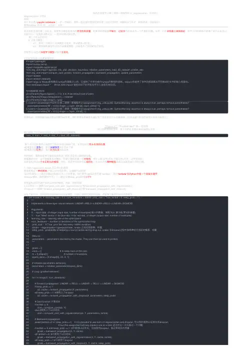
吴恩达深度学习第⼆课第⼀周编程作业_regularization(正则化)Regularization 正则化声明本⽂作业是在jupyter notebook上⼀步⼀步做的,带有⼀些过程中查找的资料等(出处已标明)并翻译成了中⽂,如有错误,欢迎指正!参考Kulbear 的和和,以及的,以及,欢迎来到本周的第⼆次作业。
深度学习模型有很⼤的灵活性和容量,如果训练数据集不够⼤,过拟合可能会成为⼀个严重的问题。
当然,它在训练集上做得很好,但学习过的⽹络不能推⼴到它从未见过的新例⼦!(也就是训练可以,⼀到实战测试就拉胯。
) 第⼆个作业的⽬的: 2. 正则化模型: 2.1:使⽤⼆范数对⼆分类模型正则化,尝试避免过拟合。
2.2:使⽤随机删除节点的⽅法精简模型,同样是为了尝试避免过拟合。
您将学习:在您的深度学习模型中使⽤正则化。
让我们⾸先导⼊将要使⽤的包。
# import packagesimport numpy as npimport matplotlib.pyplot as pltfrom reg_utils import sigmoid, relu, plot_decision_boundary, initialize_parameters, load_2D_dataset, predict_decfrom reg_utils import compute_cost, predict, forward_propagation, backward_propagation, update_parametersimport sklearnimport sklearn.datasetsimport scipy.io #scipy是构建在numpy的基础之上的,它提供了许多的操作numpy的数组的函数。
scipy.io包提供了多种功能来解决不同格式的⽂件的输⼊和输出。
from testCases import * #from XXX import*是把XXX下的所有名字引⼊当前名称空间。
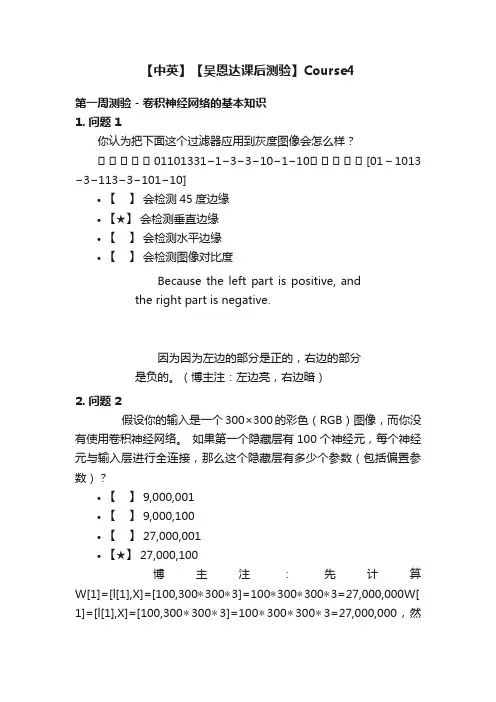
【中英】【吴恩达课后测验】Course4第一周测验 - 卷积神经网络的基本知识1. 问题 1你认为把下面这个过滤器应用到灰度图像会怎么样?⎡⎡⎡⎡⎡01101331−1−3−3−10−1−10⎡⎡⎡⎡⎡[01−1013−3−113−3−101−10]•【】会检测45度边缘•【★】会检测垂直边缘•【】会检测水平边缘•【】会检测图像对比度Because the left part is positive, andthe right part is negative.因为因为左边的部分是正的,右边的部分是负的。
(博主注:左边亮,右边暗)2. 问题 2假设你的输入是一个300×300的彩色(RGB)图像,而你没有使用卷积神经网络。
如果第一个隐藏层有100个神经元,每个神经元与输入层进行全连接,那么这个隐藏层有多少个参数(包括偏置参数)?•【】 9,000,001•【】 9,000,100•【】 27,000,001•【★】 27,000,100博主注:先计算W[1]=[l[1],X]=[100,300∗300∗3]=100∗300∗300∗3=27,000,000W[ 1]=[l[1],X]=[100,300∗300∗3]=100∗300∗300∗3=27,000,000,然后计算偏置bb,因为第一隐藏层有100个节点,每个节点有1个偏置参数,所以b=100b=100,加起来就是27,000,000+100=27,000,10027,000,000+100=27,000,100。
3. 问题 3假设你的输入是300×300彩色(RGB)图像,并且你使用卷积层和100个过滤器,每个过滤器都是5×5的大小,请问这个隐藏层有多少个参数(包括偏置参数)?•【】 2501•【】 2600•【】 7500•【★】 7600博主注:视频【1.7单层卷积网络】,05:10处。
首先,参数和输入的图片大小是没有关系的,无论你给的图像像素有多大,参数值都是不变的,在这个题中,参数值只与过滤器有关。

吴恩达深度学习笔记(5)——二分类问题二分类(Binary Classification)我们将学习神经网络的基础知识,其中需要注意的是,当实现一个神经网络的时候,我们需要知道一些非常重要的技术和技巧。
例如有一个包含m个样本的训练集,你很可能习惯于用一个for循环来遍历训练集中的每个样本(适用于有编程思维和经验的人),但是当实现一个神经网络的时候,我们通常不直接使用for循环来遍历整个训练集,所以在这周的课程中你将学会如何处理训练集。
另外在神经网络的计算中,通常先有一个叫做前向暂停(forward pause)或叫做前向传播(foward propagation)的步骤,接着有一个叫做反向暂停(backward pause) 或叫做反向传播(backward propagation)的步骤。
所以这周也会向你介绍为什么神经网络的训练过程可以分为前向传播和反向传播两个独立的部分。
在课程中我将使用逻辑回归(logistic regression)来传达这些想法,以使大家能够更加容易地理解这些概念。
即使你之前了解过逻辑回归,我认为这里还是有些新的、有趣的东西等着你去发现和了解,所以现在开始进入正题。
逻辑回归是一个用于二分类(binary classification)的算法。
二分类问题示例:首先我们从一个问题开始说起,这里有一个二分类问题的例子,假如你有一张图片作为输入,比如这只猫,如果识别这张图片为猫,则输出标签1作为结果;如果识别出不是猫,那么输出标签0作为结果(这也就是著名的cat和non cat问题)。
现在我们可以用字母y来表示输出的结果标签,如下图所示:我们来看看一张图片在计算机中是如何表示的,为了保存一张图片,需要保存三个矩阵(矩阵的概念,一定要清楚,不清楚的需要去看看线性代数了,补充下),它们分别对应图片中的红、绿、蓝三种颜色通道,如果你的图片大小为64x64像素,那么你就有三个规模为64x64的矩阵,分别对应图片中红、绿、蓝三种像素的强度值。
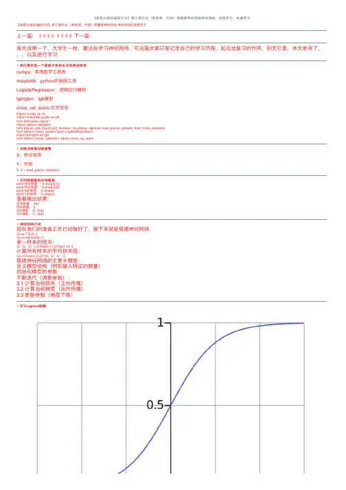
【吴恩达课后编程作业】第三周作业(附答案、代码)隐藏层神经⽹络神经⽹络、深度学习、机器学习【吴恩达课后编程作业】第三周作业(附答案、代码)隐藏层神经⽹络神经⽹络和深度学习上⼀篇:✌✌✌✌✌✌✌✌下⼀篇:⾸先说明⼀下,⼤学⽣⼀枚,最近在学习神经⽹络,写这篇⽂章只是记录⾃⼰的学习历程,起总结复习的作⽤,别⽆它意,本⽂参考了、、、以及进⾏学习✌我们要实现⼀个能够分类样本点的神经⽹络numpy:常⽤数学⼯具库matplotlib:python的画图⼯具LogisticRegression:逻辑回归模型lightgbm:lgb模型cross_val_score:交叉验证import numpy as npimport matplotlib.pyplot as pltfrom testCases import *import sklearn.datasetsfrom planar_utils import plot_decision_boundary, sigmoid, load_planar_dataset, load_extra_datasetsfrom sklearn.linear_model import LogisticRegressionimport lightgbm as lgbfrom sklearn.model_selection import cross_val_score✌加载训练测试数据集X:特征矩阵Y:标签X, Y = load_planar_dataset()✌打印数据集的详细数据print('样本数量:',X.shape[1])print('特征数量:',X.shape[0])print('X的维度:',X.shape)print('Y的维度:',Y.shape)查看输出结果:样本数量: 400特征数量: 2X的维度: (2, 400)Y的维度: (1, 400)✌神经⽹络介绍现在我们的准备⼯作已经做好了,接下来就是搭建神经⽹络\[z=w.T*X+b \]\[y=a=sigmoid(z) \]单⼀样本的损失:\[L(y,a)=-(y*log(a)+(1-y)*log(1-a)) \]计算所有样本的平均损失值:\[J=1/m\sum_{i=0}^mL(y,a) \]搭建神经⽹络的主要步骤是:定义模型结构(例如输⼊特征的数量)初始化模型的参数不断迭代(调整参数):3.1 计算当前损失(正向传播)3.2 计算当前梯度(反向传播)3.3 更新参数(梯度下降)✌定义sigmoid函数\[a=sigmoid(z) \]\[sigmoid=1/(1+e^-x) \]因为我们要做的是⼆分类问题,所以到最后要将其转化为概率,所以可以利⽤sigmoid函数的性质将其转化为0~1之间def sigmoid(z):"""功能:激活函数,计算sigmoid的值参数:z:任何维度的矩阵返回:s:sigmoid(z)"""s=1/(1+np.exp(-z))return s✌定义各⽹络层的节点数这⾥我们为什么要获取各个层的节点数呢?原因是在初始化w、b等参数时需要确定其维度,以便于后⾯的传播计算def layer_size(X,Y):"""功能:获得各个⽹络层的节点数参数:X:特征矩阵Y:标签返回:in_layer:输出层的节点数hidden_layer:隐藏层的节点数out_layer:输出层的节点数"""# 本数据集为两个特征in_layer=X.shape[0]# ⾃⼰定义隐藏层为4个节点hidden_layer=4# 输出层为1维out_layer=Y.shape[0]return in_layer,hidden_layer,out_layer✌定义初始化w、b的函数在进⾏梯度下降之前,要初始化w和b的值,但是这⾥会有个问题,为了⽅便我们会把w、b的值全部初始化为0,这样做是不正确的,原因是:如果都为0,会导致在传播计算时,模型对称,各个节点的参数不起作⽤,可以⾃⼰推到⼀下所以我们要给w、b进⾏随机取值本⽂参数维度:W1:(4,2)b1:(4,1)W2:(1,4)b2:(1,1)def init_w_b(in_layer,hidden_layer,out_layer):"""功能:初始化w,b的维度和值参数:in_layer:输出层的节点数hidden_layer:隐藏层的节点数out_layer:输出层的节点数返回:init_params:对应各层参数的字典"""# 定义随机种⼦,以便之后每次产⽣随机数唯⼀np.random.seed(2021)# 初始化参数,符合⾼斯分布W1=np.random.randn(hidden_layer,in_layer)*0.01b1=np.random.randn(hidden_layer,1)W2=np.random.randn(out_layer,hidden_layer)*0.01b2=np.random.randn(out_layer,1)init_params={'W1':W1,'b1':b1,'W2':W2,'b2':b2}return init_params✌定义向前传播函数神经⽹络分为正向传播和反向传播正向传播计算求出损失函数,然后反向计算各个梯度然后进⾏梯度下降,更新参数计算公式:\[Z1=W1*X+b1 \]\[A1=tanh(Z1) \]\[Z2=W2*A1+b2 \]\[A2=sigmoid(Z2) \]def forward(W1,b1,W2,b2,X,Y):"""功能:向前传播,计算出各个层的激活值和未激活值(A1,A2,Z1,Z2)参数:W1:隐藏层的权值参数b1:隐藏层的偏置参数W2:输出层的权值参数b2:输出层的偏置参数X:特征矩阵Y:标签返回:forward_params:对应各层数据的字典"""# 计算隐藏层Z1=np.dot(W1,X)+b1Z1=np.dot(W1,X)+b1# 激活A1=np.tanh(Z1)# 计算第⼆层Z2=np.dot(W2,A1)+b2# 激活A2=sigmoid(Z2)forward_params={'Z1':Z1,'A1':A1,'Z2':Z2,'A2':A2,'W1':W1,'b1':b1,'W2':W2,'b2':b2}return forward_params✌定义损失函数损失函数为交叉熵,数值越⼩,表明模型越优秀计算公式:\[J(W1,b1,W2,b2)=1/m\sum_{i=0}^m-(y*log(A2)+(1-y)*log(1-A2)) \]def loss_fn(W1,b1,W2,b2,X,Y):"""功能:构造损失函数,计算损失值参数:W1:隐藏层的权值参数b1:隐藏层的偏置参数W2:输出层的权值参数b2:输出层的偏置参数X:特征矩阵Y:标签返回:loss:模型损失值"""# 样本数m=X.shape[1]# 向前传播,获取激活值A2forward_params=forward(W1,b1,W2,b2,X,Y)A2=forward_params['A2']# 计算损失值loss=np.multiply(Y,np.log(A2))+np.multiply(1-Y,np.log(1-A2))loss=-1/m*np.sum(loss)# 降维,如果不写,可能会有错误loss=np.squeeze(loss)return loss✌定义向后传播函数反向计算各个梯度然后进⾏梯度下降,更新参数计算公式:\[dZ2=A2-Y \]\[dW2=1/m*dZ2*A1.T \]\[db2=1/m*\sum_{i=0}^mdZ2 \]第⼀层的参数同理,这⾥要记住计算各参数梯度,就是⾼数中的链式法则,这也就是为什么叫做向后传播,想要计算前⼀层的参数导数值就要先计算出后⼀层的梯度值\[y=2*x \]\[z=3*y \]\[∂z/∂x=(∂z/∂y )*(dy/dx) \]记住这个⼀切都OKdef backward(W1,b1,W2,b2,X,Y):"""功能:向后传播,计算各个层参数的梯度(偏导)参数:W1:隐藏层的权值参数b1:隐藏层的偏置参数W2:输出层的权值参数b2:输出层的偏置参数X:特征矩阵Y:标签返回:grads:各参数的梯度值"""# 样本数m=X.shape[1]# 进⾏前向传播,获取各参数值forward_params=forward(W1,b1,W2,b2,X,Y)A1=forward_params['A1']A2=forward_params['A2']W1=forward_params['W1']W2=forward_params['W2']# 计算梯度dZ2= A2 - YdW2 = (1 / m) * np.dot(dZ2, A1.T)db2 = (1 / m) * np.sum(dZ2, axis=1, keepdims=True)dZ1 = np.multiply(np.dot(W2.T, dZ2), 1 - np.power(A1, 2))dW1 = (1 / m) * np.dot(dZ1, X.T)db1 = (1 / m) * np.sum(dZ1, axis=1, keepdims=True)grads = {"dW1": dW1,"db1": db1,"dW2": dW2,"db2": db2 }return grads✌定义整个传播过程⼀个传播流程包括:向前传播计算损失函数向后传播3.1 计算梯度3.2 更新参数def propagate(W1,b1,W2,b2,X,Y):"""功能:传播运算,向前->损失->向后->参数:W1:隐藏层的权值参数b1:隐藏层的偏置参数W2:输出层的权值参数b2:输出层的偏置参数X:特征矩阵Y:标签Y:标签返回:grads,loss:各参数的梯度,损失值"""# 计算损失loss=loss_fn(W1,b1,W2,b2,X,Y)# 向后传播,计算梯度grads=backward(W1,b1,W2,b2,X,Y)return grads,loss✌定义优化器函数⽬标是通过最⼩化损失函数 J来学习 w 和 b 。
深度学习基础知识题库1. 什么是深度学习?深度学习是一种机器学习方法,通过使用多层神经网络来模拟人脑的工作原理,从而实现对数据进行学习和分析的能力。
深度学习模型通常由多层神经网络组成,每一层都对输入数据进行特征提取和转换,最终输出预测结果。
2. 深度学习与传统机器学习的区别是什么?深度学习与传统机器学习的主要区别在于特征提取的方式和模型的复杂度。
传统机器学习方法需要手工选择和设计特征,而深度学习可以自动从原始数据中学习最有用的特征。
此外,深度学习模型通常比传统机器学习模型更复杂,拥有更多的参数需要训练。
3. 请解释下面几个深度学习中常用的概念:神经网络、激活函数和损失函数。
•神经网络是深度学习的核心组成部分,它由多个神经元组成,并通过神经元之间的连接进行信息传递和处理。
每个神经元接收一组输入,并通过激活函数对输入进行非线性转换后输出结果。
•激活函数是神经网络中的一个重要组件,主要用于引入非线性。
常用的激活函数包括Sigmoid、ReLU和tanh,它们可以将神经网络的输出限制在一定的范围内,并增加模型的表达能力。
•损失函数用于衡量模型的预测结果与真实标签之间的差异。
常见的损失函数包括均方误差(MSE)、交叉熵(Cross-Entropy)等,模型的目标是通过优化损失函数的数值来提高预测的准确性。
4. 请解释一下反向传播算法在深度学习中的作用。
反向传播算法是深度学习中训练神经网络的关键算法之一。
它基于梯度下降的思想,通过计算当前预测值和真实标签之间的差异,并向后逐层更新神经网络中的参数,从而最小化误差。
具体地,反向传播算法沿着神经网络的前向传播路径,依次计算每一层的导数和误差。
然后使用链式法则将误差从输出层逐层向后传播,更新每个神经元的参数,直到最后一层。
反向传播算法的使用可以加速神经网络训练的过程,提高模型的准确性。
5. 请简要介绍一下卷积神经网络(CNN)以及它在计算机视觉任务中的应用。
卷积神经网络(Convolutional Neural Network,CNN)是一种深度学习模型,特别适用于处理网格状数据,如图像和语音。
【吴恩达深度学习】优化算法–Sniper吴恩达深度学习第二课第二周优化方法1.mini-batch梯度下降假如我们有一个长度为500w的数据集,这时候我们如果要做梯度下降,每下降一次需要对500w长度的向量进行计算。
这时候我们引入mini-batch算法,假设我们将每批设为1000个长度,这时候我们可以将整个数据分成5000份(结果集同理),命名规则如下然后使用for循环,对每1000个数据进行一次梯度下降,这样我们500w条数据可以进行5000次下降,提高了收敛速度。
2.理解mini-batch梯度下降算法如果我们在batch梯度下降法中遇到了代价上升的问题,说明我们的学习率过大。
而如果我们使用mini-batch算法,这却是正常的。
在mini-batch中,不是每次迭代代价都会下降,因为每次迭代中处理的都是不同的样本,因此十分可能我们最终得到的代价曲线是一个如下图的样子但是我们需要注意,虽然有起伏是无所谓的,但是整体的走势应该是向下的。
噪声的产生是因为可能当前的parameters对某一批的拟合程度比较好或者当前批的数据有一些残缺值等,因此代价会起伏变化。
你需要决定的变量之一是mini-batch大小,m就是训练集的大小,在极端的情况下,mini-batch大小等于m,那么就退化成了batch梯度下降法;另一种极端是mini-batch的大小为1,这时候就成了另一种算法——随机梯度下降法,既每一个样本都是mini-batch。
对于batch梯度下降法和随机梯度下降法,有如下图我们看到,随机梯度下降法并不会一直向着最好的方向前进,但是总体趋势是下降的,并且最后不会收敛到某一个具体值,而是在某一值附近浮动,而mini-batch虽然后浮动但是波动不大,总体上较快的逼近收敛值。
如果训练集较小则可以直接使用batch梯度下降法(一般指2000以内)。
大小一般为2的n次方倍。
一方面,充分利用的GPU的并行性,另一方面,不会让计算时间特别长3.指数加权平均数我们假定全年的温度数据如下我们使用前一天的温度*0.9+今天的温度*0.1,然后就可以画出下面的曲线我们将上面的式子推广到一般情况我们发现上面我们取0.9的时候,实际上是今天的天气权重只有0.1,之前的天气权重为0.9,这样相当于计算了10天的平均气温。
吴恩达机器学习作业2-逻辑回归与正则化作业(python实现)机器学习练习2 python复现- 逻辑回归在此练习中,需要实现逻辑回归应⽤于分类任务。
还通过将正则化加⼊训练算法中来提⾼算法的鲁棒性,并⽤更复杂的情形进⾏测试。
逻辑回归在训练的初始阶段,我们将要构建⼀个逻辑回归模型来预测,某个学⽣是否被⼤学录取。
设想你是⼤学相关部分的管理者,想通过申请学⽣两次测试的评分,来决定他们是否被录取。
现在你拥有之前申请学⽣的可以⽤于训练逻辑回归的训练样本集。
对于每⼀个训练样本,你有他们两次测试的评分和最后是被录取的结果。
为了完成这个预测任务,我们准备构建⼀个可以基于两次测试评分来评估录取可能性的分类模型。
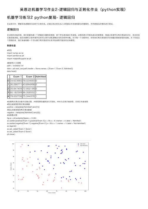
数据检查#导包import numpy as npimport pandas as pdimport matplotlib.pyplot as plt#数据导⼊与查看path = 'ex2data1.txt'data = pd.read_csv(path,header = None,names = ['Exam 1','Exam 2','Admitted'])data.head()Exam 1Exam 2Admitted034.62366078.0246930130.28671143.8949980235.84740972.9021980360.18259986.3085521479.03273675.3443761#创建两次测试分数对应散点图,并使⽤颜⾊编码进⾏可视化,样本为正表⽰被录取,负表⽰未被录取#取出被录取的两次测试数据positive = data[data['Admitted'].isin([1])]#取出未被录取的两次测试数据negative = data[data['Admitted'].isin([0])]#绘制散点图fig,ax = plt.subplots(figsize = (12,8))ax.scatter(positive['Exam 1'],positive['Exam 2'],s = 50,c = 'b',marker = 'o',label = 'Admitted')ax.scatter(negative['Exam 1'],negative['Exam 2'],s = 50,c = 'r',marker = 'x',label = 'Not Admitted')ax.legend()ax.set_xlabel('Exam 1 Score')ax.set_ylabel('Exam 2 Score')plt.show()观察可以发现两类间有清晰的决策边界,现在我们需要实现逻辑回归,就可以训练⼀个模型来预测结果。
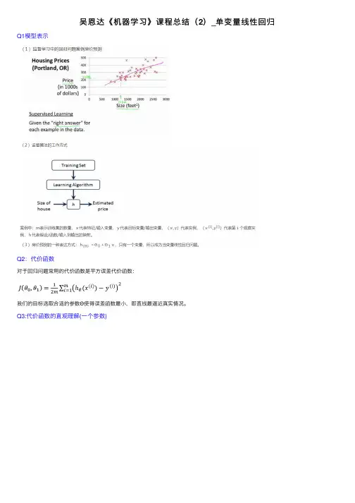
吴恩达《机器学习》课程总结(2)_单变量线性回归Q1模型表⽰
Q2:代价函数
对于回归问题常⽤的代价函数是平⽅误差代价函数:
我们的⽬标选取合适的参数Θ使得误差函数最⼩,即直线最逼近真实情况。
Q3:代价函数的直观理解(⼀个参数)
Q4:代价函数的直观理解(两个参数)
Q5梯度下降
Q6梯度下降的直观理解
(1)梯度下降法可以最⼩化任何代价函数,⽽不仅仅局限于线性回归中的代价函数。
(2)当越来越靠近局部最⼩值时,梯度值会变⼩,所以即使学习率不变,参数变化的幅度也会随之减⼩。
(3)学习率过⼩时参数变化慢,到达最优点的时间长,学习率⼤时,可能导致代价函数⽆法收敛,甚⾄发散。
(4)梯度就是某⼀点的斜率。
Q7梯度下降的线性回归
英语词汇
Linear regression with one variable ---单变量线性回归model representation ---模型表⽰
training set ---训练集
hypothesis ---假设
gradient descent ---梯度下降
convergence ---收敛
local minimum ---局部最⼩值
global minimum ---全局最⼤值。
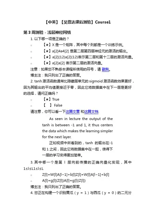
【中英】【吴恩达课后测验】Course1第3周测验 - 浅层神经网络1.以下哪一项是正确的?o【★】X是一个矩阵,其中每个列都是一个训练示例。
o【★】a[2]4a4[2] 是第二层第四层神经元的激活的输出。
o【★】a[2](12)a[2](12)表示第二层和第十二层的激活向量。
o【★】a[2]a[2] 表示第二层的激活向量。
注意:如果您不熟悉本课程所使用的符号,请戳我。
博主注:我只列出了正确的答案。
2.tanh激活函数通常比隐藏层单元的sigmoid激活函数效果更好,因为其输出的平均值更接近于零,因此它将数据集中在下一层是更好的选择,请问正确吗?o【★】Trueo【】 False请注意,你可以看一下这篇文章和这篇文档.As seen in lecture the output of thetanh is between -1 and 1, it thus centersthe data which makes the learning simplerfor the next layer.正如视频中所看到的,tanh的输出在-1和1之间,因此它将数据集中在一起,使得下一层的学习变得更加简单。
3.其中哪一个是第l层向前传播的正确向量化实现,其中1≤l≤L1≤l≤Lo Z[l]=W[l]A[l−1]+b[l]Z[l]=W[l]A[l−1]+b[l]o A[l]=g[l](Z[l])A[l]=g[l](Z[l])博主注:我只列出了正确的答案。
4.您正在构建一个识别黄瓜(y = 1)与西瓜(y = 0)的二元分类器。
你会推荐哪一种激活函数用于输出层?o【】 ReLUo【】 Leaky ReLUo【★】sigmoido【】 tanh注意:来自sigmoid函数的输出值可以很容易地理解为概率。
Sigmoid outputs a value between 0and 1 which makes it a very good choicefor binary classification. You can classify as0 if the output is less than 0.5 and classifyas 1 if the output is more than 0.5. It canbe done with tanh as well but it is lessconvenient as the output is between -1and 1.Sigmoid输出的值介于0和1之间,这使其成为二元分类的一个非常好的选择。
吴恩达深度学习笔记⽬录吴恩达讲深度学习为什么要学习深度学习1.数据量更⼤2.算法越来越优3.业务场景越来越多样化4.学术界or⼯业界越来越卷(私以为!)从逻辑回归讲起逻辑回归是最简单的⼆分类模型,也可以说是后续深度神经⽹络的基础框架.达叔的算法知识第⼀课.逻辑回归的参数是W和b,也是主要学习的参数矩阵\hat{y}=\sigma\left(w^{T} x+b\right), where \sigma(z)=\frac{1}{1+e^{-z}}Given \left\{\left(x^{(1)}, y^{(1)}\right), \ldots,\left(x^{(m)}, y^{(m)}\right)\right\}, want \hat{y}^{(i)} \approx y^{(i)}损失函数/误差函数主要是衡量单⼀样例的模型训练效果的,希望模型得到的\hat{y}^{(i)}是⽆限趋近于实际的值y^{(i)},⼆成本函数是⽤来衡量参数w和参数b的效果的.\begin{array}{c} \text { Recap: } \hat{y}=\sigma\left(w^{T} x+b\right), \sigma(z)=\frac{1}{1+e^{-z}}< \\ J(w, b)=\frac{1}{m} \sum_{i=1}^{m} \mathcal{L}\left(\hat{y}^{(i)}, y^{(i)}\right)=-\frac{1}{m} \sum_{i=1}^{m} y^{(i)} \log \hat{y}^{(i)}+\left(1-y^{(i)}\right) \log \left(1-\hat{y}^{(i)}\right) \end{array}逻辑回归的梯度下降z=w^{T} x+b\hat{y}=a=\sigma(z)\mathcal{L}(a, y)=-(y \log (a)+(1-y) \log (1-a))导数的细节函数的导数就是函数的斜率向量化为什么要向量化实现,因为对⽐for循环来说,向量化的⽅式可以⼤⼤减⼩运⾏时间。
《深度学习》课后习题,,,,10《深度学习》课后习题逻辑回归模型与神经网络 - 逻辑回归模型与神经网络 - 深度学习 1.机器学习中模型的训练误差和测试误差是一致的。
* A .对 B .错正确答案:B 2.机器学习中选择的模型越复杂越好。
* A .对 B .错正确答案:B 3.解决模型过拟合问题的一个方法是正则化。
* A .对 B .错正确答案:A 4.模型在训练阶段的效果不太好称之为欠拟合。
* A .对 B .错正确答案:A 5.如果模型的误差于偏差较大,可以采用以下措施解决。
* A .给数据增加更多的特征 B .设计更复杂的模型 C .增加更多的数据 D .使用正则化正确答案:A,B 6.如果模型的误差于偏差较大,可以采用以下措施解决* A .给数据增加更多的特征 B .设计更复杂的模型C .增加更多的数据 D .使用正则化正确答案:A,B 深度学习概述- 深度学习概述 - 深度学习 1.一个神经元的作用相当于一个逻辑回归模型。
* A .对 B .错正确答案:A 2.神经网络可以看成由多个逻辑回归模型叠加而成。
* A .对 B .错正确答案:A 3.神经网络的参数由所有神经元连接的权重和偏差组成。
* A .对 B .错正确答案:A 4.一个结构确定的神经网络对应一组函数 ___,而该神经网络的参数确定后就只对应一个函数。
* A .对B .错正确答案:A 5.深度神经网络的深度一般是网络隐藏层的数量。
* A .对 B .错正确答案:A 6.神经网络从计算上可以看成矩阵运算和非线性运算的多次叠加而组成的复合函数,且网络叠加的层次可看成复合函数的嵌套深度。
* A .对 B .错正确答案:A 7.神经网络的层次和每层神经元的数量可以通过以下哪些方法确定?* A .可随意设定 B .可人为进行设计 C .可通过进化算法学习出来 D .可通过强化算法学习出来正确答案:B,C,D 8.深度学习兴起的标志性 ___包括。
深度学习——1×1卷积核理解1 - 引⼊ 在我学习吴恩达⽼师Deeplearning.ai深度学习课程的时候,⽼师在第四讲卷积神经⽹络第⼆周深度卷积⽹络:实例探究的2.5节⽹络中的⽹络以及1×1卷积对1×1卷积做了较为详细且通俗易懂的解释。
现⾃⼰做⼀下记录。
2 - 1×1卷积理解 假设当前输⼊张量维度为6×6×32,卷积核维度为1×1×32,取输⼊张量的某⼀个位置(如图黄⾊区域)与卷积核进⾏运算。
实际上可以看到,如果把1×1×32卷积核看成是32个权重$W$,输⼊张量运算的1×1×32部分为输⼊$x$,那么每⼀个卷积操作相当于⼀个$Wx$过程,多个卷积核就是多个神经元,相当于⼀个全连接⽹络。
综上,可以将1×1卷积过程看成是将输⼊张量分为⼀个个输⼊为1×1×32的$x$,他们共享卷积核变量(对应全连接⽹络的权重)$W$的全连接⽹络。
3 - 1×1卷积核作⽤3.1 - 放缩$n_c$的⼤⼩ 通过控制卷积核的数量达到通道数⼤⼩的放缩。
⽽池化层只能改变⾼度和宽度,⽆法改变通道数。
3.2 - 增加⾮线性 如上所述,1×1卷积核的卷积过程相当于全连接层的计算过程,并且还加⼊了⾮线性激活函数,从⽽可以增加⽹络的⾮线性,使得⽹络可以表达更加复杂的特征。
3.3 - 减少参数 在Inception Network中,由于需要进⾏较多的卷积运算,计算量很⼤,可以通过引⼊1×1确保效果的同时减少计算量。
具体可以通过下⾯例⼦量化⽐较。
3.3.1 - 不引⼊1×1卷积的卷积操作 总共需要的计算量为(28×28×32)×(5×5×192)≈ 120 million3.3.2 - 引⼊1×1卷积的卷积操作 总共需要的计算量为(28×28×16)×(1×1×192)+(28×28×32)×(5×16×16)≈ 12.4 million,明显少于不引⼊1×1卷积的卷积过程的计算量。
2-1 分析为什么平方损失函数不适用于分类问题?损失函数是一个非负实数,用来量化模型预测和真实标签之间的差异。
我们一般会用损失函数来进行参数的优化,当构建了不连续离散导数为0的函数时,这对模型不能很好地评估。
直观上,对特定的分类问题,平方差的损失有上限(所有标签都错,损失值是一个有效值),但交叉熵则可以用整个非负域来反映优化程度的程度。
从本质上看,平方差的意义和交叉熵的意义不一样。
概率理解上,平方损失函数意味着模型的输出是以预测值为均值的高斯分布,损失函数是在这个预测分布下真实值的似然度,softmax 损失意味着真实标签的似然度。
在二分类问题中y = { + 1 , − 1 }在C 分类问题中y = { 1 , 2 , 3 , ⋅ ⋅ ⋅ , C }。
可以看出分类问题输出的结果为离散的值。
分类问题中的标签,是没有连续的概念的。
每个标签之间的距离也是没有实际意义的,所以预测值和标签两个向量之间的平方差这个值不能反应分类这个问题的优化程度。
比如分类 1,2,3, 真实分类是1, 而被分类到2和3错误程度应该是一样的,但是明显当我们预测到2的时候是损失函数的值为1/2而预测到3的时候损失函数为2,这里再相同的结果下却给出了不同的值,这对我们优化参数产生了误导。
至于分类问题我们一般采取交叉熵损失函数(Cross-Entropy Loss Function )来进行评估。
2-2 在线性回归中,如果我们给每个样本()()(,)n n x y 赋予一个权重()n r ,经验风险函数为()()()211()()2N n n T n n R w r y w x ==−∑,计算其最优参数*w ,并分析权重()n r 的作用.答:其实就是求一下最优参数*w ,即导数为0,具体如下:首先,取权重的对角矩阵:()(),,,n P diag r x y w =均以向量(矩阵)表示,则原式为:21()||||2T R P Y X Ω=−Ω ,进行求导:()0T R XP Y X ∂=−−Ω=∂Ω,解得:*1()T XPX XPY −Ω=,相比于没有P 时的Ω:1()T withoutP XX XY −Ω=,可以简单理解为()n r 的存在为每个样本增加了权重,权重大的对最优值ω的影响也更大。
单选题(每题1分,共39道题)1、[单选]你让一些人对数据集进行标记,以便找出人们对它的识别度。
你发现了准确度如下:鸟类专家1 0.3%Error〔误差〕鸟类专家2 0.5%Error〔误差〕普通人1 1.0%Error〔误差〕普通人2 1.2%Error〔误差〕如果您的目标是将“人类表现”作为贝叶斯错误的基准线(或估计),那么您如何定义“人类表现”?• A:0.0%〔因为不可能做得比这更好〕• B:0.3%(专家1的错误率〕• C:0.4%〔0_3到0.5之间〕• D:0.75%〔以上所有四个数字的平均值〕正确答案:B你的答案:B解析:“人类表现”的定义通常是指人类能够达到的最佳表现水平,而鸟类专家1的错误率是所有人中最低的,因此人类表现应该是以其错误率作为基准线,即选项B:0.3%。
2、[单选]你有一个32x32x16的输入,并使用步幅为2、过滤器大小为2的最大池化,请问输出是多少?• A:15x15x16• B:16x16x8• C:16x16x16• D:32x32x8正确答案:C你的答案:C解析:使用步幅为2的最大池化,输出的大小会缩小一半,因此输出为16x16x16。
因此选项C为正确答案。
3、[单选]以下有关特征数据归一化的说法错误的是:• A:特征数据归一化加速梯度下降优化的速度• B:特征数据归一化有可能提高模型的精度• C:线性归一化适用于特征数值分化比较大的情况• D:概率模型不需要做归一化处理正确答案:C你的答案:C解析:特征数据归一化可以加速梯度下降优化的速度,因此A正确;数据的归一化有可能让模型更容易收敛从而提高精度,故B正确。
线性归一化适用于数值比较集中的情况,因此C选项错误。
特征数值分化比较大的情况。
概率模型不需要归一化,因为它们不关心变量的值,而是关心变量的分布和变量之间的条件概率,如决策树、随机森林,因此D选项正确。
综上所述,答案为C。
4、[单选]在CNN网络中,图A经过核为3x3,步长为2的卷积层,ReLU激活函数层,BN层,以及一个步长为2,核为2*2的池化层后,再经过一个3*3的的卷积层,步长为1,此时的感受野是()• A:10• B:11• C:12• D:13正确答案:D你的答案:D解析:感受野的计算公式为:RF=(N_RF - 1) * stride + kernel,其中,RF是感受野,N_RF和RF有点像,N代表 neighbour,指的是第n层的一个特征点在n-1层的RF。
吴恩达深度学习第⼆课第三周编程作业_TensorFlowTutorialTensorFlow教程TensorFlow Tutorial TensorFlow教程欢迎来到本周的编程作业。
到⽬前为⽌,您⼀直使⽤numpy来构建神经⽹络。
现在我们将引导你通过⼀个深度学习框架,它将允许你更容易地建⽴神经⽹络。
像TensorFlow, PaddlePaddle, Torch, Caffe, Keras等机器学习框架可以显著加快你机器学习的发展。
所有这些框架都有⼤量⽂档,您可以随意阅读。
在这个作业中,你将学习在TensorFlow中完成以下操作:初始化变量开始你⾃⼰的会话训练算法实现⼀个神经⽹络编程框架不仅可以缩短您的编码时间,有时还可以执⾏优化来加速您的代码。
1 - Exploring the Tensorflow Library 探索Tensorflow库⾸先,您将导⼊库:1 import math2 import numpy as np3 import h5py4 import matplotlib.pyplot as plt5 import tensorflow as tf6 from tensorflow.python.framework import ops7 from tf_utils import load_dataset, random_mini_batches, convert_to_one_hot, predict89 %matplotlib inline10 np.random.seed(1)现在您已经导⼊了库,我们将带您浏览它的不同应⽤程序。
你将从⼀个例⼦开始,我们计算⼀个训练例⼦的损失。
原代码为:y_hat = tf.constant(36, name='y_hat') # Define y_hat constant. Set to 36.y = tf.constant(39, name='y') # Define y. Set to 39loss = tf.Variable((y - y_hat)**2, name='loss') # Create a variable for the lossinit = tf.global_variables_initializer() # When init is run later (session.run(init)),# the loss variable will be initialized and ready to be computedwith tf.Session() as session: # Create a session and print the outputsession.run(init) # Initializes the variablesprint(session.run(loss)) # Prints the loss根据⽹上参考,适应tf2.0版本修改的:import tensorflow as tfpat.v1.disable_eager_execution() #保证session.run()能够正常运⾏y_hat = tf.constant(36, name='y_hat') # Define y_hat constant. Set to 36.y = tf.constant(39, name='y') # Define y. Set to 39loss = tf.Variable((y - y_hat)**2, name='loss') # Create a variable for the lossinit = pat.v1.global_variables_initializer() # When init is run later (session.run(init)),# the loss variable will be initialized and ready to be computedwith pat.v1.Session () as session: # Create a session and print the outputsession.run(init) # Initializes the variablesprint(session.run(loss))运⾏结果:在TensorFlow中编写和运⾏程序有以下步骤:1、创建Tensorflow变量(此时,尚未直接计算)2、实现Tensorflow变量之间的操作定义。
《吴恩达-机学》⼀、回归、分类、监督学习、⾮监督学习1 ) Well-posed learning problem : A computer program is said to learn from experience E with respect to(关于) some task T and some performance measure(测量) P, if its performance on T, as measured by P, improves with experience E.适当的学习问题构成:⼀个电脑程序从经验E中学习去解决某⼀任务T,进⾏某⼀性能测量P,通过P测定在T上的表现,因经验E⽽提⾼总结,机器学习三要素:E,T,P====================================例⼦:对于跳棋,经验:⾃⼰和⾃⼰下成千上万次任务:玩跳棋表现:和对⼿玩成功概率Q: Suppose your email program watches which emails you do or do not mark as spam, and based on that learns how to betterfilter spam. What is the task T in this setting?(A). Classifying emails as spam or not spam.------这个是T,是我们想要达成的任务,⽬标。
(B). Watching you label emails as spam or not spam. ------ 这个是E,可以说是积攒的经验,也就是学习的过程。
(C). The number (or fraction分数) of emails correctly classified as spam/not spam. ----- 这个是P,相当于来个学习的总结或者评价,看正确分类的数量或者⽐例。
Practical aspects of deep learning1.If you have 10,000,000 examples, how would you split the train/dev/test set?☐33% train, 33% dev, 33% test☐60% train, 20% dev, 20% test☐98% train, 1% dev, 1% test2.The dev and test set should:☐Come from the same distribution☐Come from different distribution☐Be identical to each other (same (x,y) pairs)☐Have the same number of examples3.If your Neural Network model seems to have high bias, what of the following would bepromising things to try? (Check all that apply.)☐Add regularization☐Get more test data☐Increase the number of units in each hidden layer☐Make the Neural Network deeper☐Get more training data4.You are working on an automated check-out kiosk for a supermarket, and are building aclassifier for apples, bananas and oranges. Suppose your classifier obtains a training set error of 0.5%, and a dev set error of 7%. Which of the following are promising things to try to improve your classifier? (Check all that apply.)☐Increase the regularization parameter lambda☐Decrease the regularization parameter lambda☐Get more training data☐Use a bigger neural network5.What is weight decay?☐ A regularization technique (such as L2 regularization) that results in gradient decent shrinking the weights on every iteration.☐The process of gradually decreasing the learning rate during training.☐Gradual corruption of the weights in the neural network if it is trained on noisy data.☐ A technique to avoid vanishing gradient by imposing a ceiling on the values of the weights.6.What happens when you increase the regularization hyperparameter lambda?☐Weights are pushed toward becoming smaller (closer to 0)☐Weights are pushed toward becoming bigger (further from 0)☐Doubling lambda should roughly result in doubling the weights☐Gradient descent taking bigger steps with each iteration (proportional to lambda)7.With the inverted dropout technique, at test time:☐You apply dropout (randomly eliminating units) and do not keep the 1/keep_prob factor in the calculations used in training☐You apply dropout (randomly eliminating units) but keep the 1/keep_prob factor in the calculations used in training.☐You do not apply dropout ( do not randomly eliminating units), but keep the 1/keep_prob factor in the calculations used in training.☐You do not apply dropout (do not randomly eliminating units) and do not keep the 1/keep_prob factor in the calculations used in training.8.Increasing the parameter keep_prob from (say) 0.5 to 0.6 will likely cause the following:(Check the two that apply)☐Increasing the regularization effect☐Reducing the regularization effect☐Causing the neural network to end up with a higher training set error☐Causing the neural network to end up with a lower training set error9.Which of these techniques are useful for reducing variance (reducing overfitting)? (Check allthat apply.)☐Xavier initialization☐Data augmentation☐Gradient Checking☐Exploding gradient☐L2 regularization☐Vanishing gradient☐Dropout10.Why do we normalize the inputs x?☐It makes the parameter initialization faster☐It makes the cost function faster to optimize☐Normalization is another word for regularization—It helps to reduce variance☐It makes it easier to visualize the dataOptimization algorithms1.Which notation would you use to denote the 3rd layer’s activation when the inputs is the 7thexample from the 8th minibatch?☐a[8]{3}(7)☐a[8]{7}(3)☐a[3]{8}(7)☐a[3]{7}(8)2.Which of these statements about mini-batch gradient descent do you agree with ?☐One iteration of mini-batch gradient decent (computing on a single mini-batch) is faster than one iteration of batch gradient decent.☐You should implement mini-batch gradient descent without an explicit for loop over different mini-batches, so that the algorithm processes all mini-batches at the same time (vectorization).☐Training one epoch (one pass through the training set) using mini-batch gradient descent is faster than training one epoch using batch gradient descent.3.Why is the best mini-batch size usually not 1 and not m, but instead something in-between?☐If the mini-batch size is m, you end up with stochastic gradient descent, which is usually slower than mini-batch gradient descent.☐If the mini-batch size is m, you end up with batch gradient descent, which has to process the whole training set before making progress.☐If the mini-batch size is 1, you lose the benefits of vectorization across examples in the mini-batch.☐If the mini-batch size is 1, you end up having to process the entire training set before making any progress.4.Suppose your learning algorithm’s cost J, plotted as a function of the number of iterations,looks like this:Which of the following do you agree with?☐Whether you’re using batch gradient decent or mini-batch gradient decent, something is wrong.☐Whether you’re using batch gradient decent of mini-batch gradient descent, this looks acceptable.☐If you’re using mini-batch gradient descent, something is wrong. But if you’re using batch gradient descent, this looks acceptable.☐If you’re using mini-batch gradient descent, this looks acceptable. But if you’re using batch gradient decent, something is wrong.5.Suppose the temperature in Casablanca over the first three days of January are the same:Jan 1st: θ1=100CJan 2nd: θ2=100C(We used Fahrenheit in lecture, so will use Celsius here in honor of the metric world.)Say you use an exponentially weighted average with β=0.5 to track the temperature:v0=0, v t=βv t-1+(1-β)θt. If v2 is the value computed after day 2 without bias correction, and v2corrected is the value you compute with bias correction. What are these values? (You might be able to do this without a calculator, but don’t actually need one. Remember what is bias correction doing.)☐v2=7.5, v2corrected=10☐v2=10, v2corrected=7.5☐v2=7.5, v2corrected=7.5☐v2=10, v2corrected=106.Which of these is NOT a good learning rate decay scheme? Here, t is the epoch number.☐α=1α01+2∗t☐α=e tα0☐α=0.95tα0☐α=α0√t7.You use an exponentially weighted average on the London temperature dataset. You use thefollowing to track the temperature: v t=βv t-1+(1-β)θt. The red line below was computed using β=0.9. What would happen to your red curve as you vary β? (Check the two that apply)☐Decreasing βwill shift the red line slightly to the right☐Increasing βwill shift the red line slightly to the right☐Decreasing βwill create more oscillation within the red line.☐Increasing βwill create more oscillation within the red line.8.Consider this figure:These plots were generated with gradient descent; with gradient descent momentum (β=0.5) and gradient descent with momentum (β=0). Which curve corresponds to whichalgorithm?☐(1) is gradient descent with moment (small β). (2) is gradient descent. (3) is gradient descent with momentum (large β)☐(1) is gradient descent. (2) is gradient descent with momentum (small β). (3) is gradient descent with momentum (large β)☐(1) is gradient descent. (2) is gradient descent with momentum (large β). (3) is gradient descent with momentum (small β)☐(1) is gradient descent with momentum (small β). (2) is gradient descent with momentum (small β). (3) is gradient descent.9.Suppose batch gradient descent in a deep network is taking excessively long to find a value ofthe parameters that achieves a small value for the cost function J(W[1],b[1],……,W[L],b[L]).Which of the following techniques could help find parameter values that attain a small value for J? (check all that apply)☐Try tuning the learning rate α☐Try initializing all the weights to zero☐Try better random initialization for the weights☐Try mini-batch gradient descent☐Try using Adam10.Which of the following statements about Adam is False?☐Adam combines the advantages of RMSProp and momentum☐Adam should be used with batch gradient computations, not with mini-batches.☐The learning rate hyperparameter αin Adam usually needs to be tuned.☐We usually use “default” values for the hyperparameter β1, β2 andεin Adam (β=0.9, β2=0.999, ε=10-8)1Hyperparameter tuning, Batch Normalization, Programming Frameworks1.If searching among a large number of number of hyperparameters, you should try values in agrid rather than random values, so that you can carry out the search more systematically and not rely on chance. True or False?☐True☐False2.Every hyperparameters, if set poorly, can have a huge negative impact on training, and so allhyperparameters are about equally important to tune well. True or False?☐True☐False3.During hyperparameters serch, whether you try to babysit one model (“Panda” strategy) ortrain a lot of models in parallel (“Caviar”) is largely determined by:☐Whether you use batch or mini-batch optimization☐The presence of local minima (and saddle points) in your neural network☐The amount of computational power you can access☐The number of hyperparameters you have to tune4.If you think β(hyperparameter for momentum) is between on 0.9 and 0.99, which of thefollowing is the recommended way to sample a value for beta?☐ 1 r = np.random.rand()2 beta = r*0.09+0.09☐ 1 r = np.random.rand()2 beta = 1-10**(-r-1)☐ 1 r = np.random.rand()2 beta = 1-10**(-r+1)☐ 1 r = np.random.rand()2 beta = r*0.9+0.095.Finding good hyperparameter values is very time-consuming. So typically you should to itonce at the start of the project, and try to find very good hyperparameters so that you don’t ever have to revisit tuning them again. True or False?☐True☐False6.In batch normalization as presented in the video, if you apply it on the l th layer of you neuralnetwork, what are you normalizing?☐B [l ] ☐a [l ] ☐Z [l ] ☐W [l ]7. In the normalization formula z norm (i)=(i)√σ2+ε, why do we use epsilon?☐To speed up convergence ☐To avoid division by zero ☐To have a more accurate normalization ☐In case μ is too small8. Which of the following statements about γ and β in Batch Norm are true?☐ There is one global value of γ∈R and one global value of β∈R for each layer, andapplies to all the hidden units in that layer.☐ They can be learned using Adam, Gradient descent with momentum, or RMSprop, notjust with gradient descent.☐ The optimal values are γ=√σ2+ϵ, and β=μ.☐ β and γ are hyperparameters of the algorithm, which we tune via random sampling. ☐ They set the mean and variance of the linear variable z [l] of a given layer.9. After training a neural network with Batch Norm, at test time, to evaluate the neural networkon a new example you should:☐ Perform the needed normalization, use μ and σ2 estimated using an exponentiallyweighted average across mini-batches seen during training.☐ Skip the step where you normalize using μ and σ2 since a single test example cannotbe normalized☐ Use the most recent mini-batch ’s value of μ and σ2 to perform the needednormalizations.☐ If you implemented Batch Norm on mini-batches of (say) 256 examples, then toevaluate on one test example, duplicate that example 256 time so that you ’re working with a mini-batch the same size as during training.10. Which of these statements about deep learning programming frameworks are true? (Checkall that apply)☐ A programming frameworks allows you to code up deep learning algorithms withtypically fewer lines of code than a lower-level language such as Python.☐ Even if a project is currently open source, good governance of the project helps ensurethat the it remains open even in the long term, rather than become closed or modified to benefit only one company.Deep learning programming frameworks require cloud-based machines to run.。