T-DOF PI Controller Design for a Speed Control of Induction Motor

自由度用英语怎么说在当今时代的电子游戏中，也有自由度这个概念，在高自由度的游戏中，玩家可以不必一定要按照规定的路线进行。

玩家操作人物在地图中可以向各个方向前进、做事，受到的拘束很少。

那么你知道自由度用英语怎么说吗?下面店铺为大家带来自由度的英语说法，供大家学习。

自由度的英语说法1：freedom自由度的英语说法2：free degree自由度相关英语表达：多自由度系统 many degrees of freedom system六自由度 six degrees of freedom单自由度系统 Single Degree-Of-Freedom System无效自由度 passive degree of freedom自由度的英语例句：1. With some limitations, this is true also of rotational degrees of freedom.在某些限定条件下, 这一说法对转动自由度也成立.2. The results converge reasonably well for the twelve degress of freedom case.对于十二个自由度的情形来说,结果收敛得相当好.3. In a three - body decay, the emerging particles have more freedom.在三体衰变中, 出现的产物粒子有较大的自由度.4. Each F distribution has a pair of degrees of freedom.每个F分布,都有一对自由度.5. It imposes constrains, restricting nature's freedom.它具有限制自然界自由度的强制性.6. The internal degrees of freedom are almost, but not completely, frozen out of the energy sharing.内自由度几乎都与能量分配无关, 但并非全部无关.7. A single - degree - of - freedom rate gyro can be made to indicate north, provided that it is sensitive enough.如果单自由度速率陀螺具有足够的灵敏度,就可以用它来指示北向.8. For a system comprising two or more objects, degrees of freedom are additive.具有两个或更多个物体的系统, 自由度更多.9. Thus a 2 - freedom - degree mechanic model for dynamic tension was constructed.基于这些结果建立了两自由度动张力模型.10. A new 6 - DOF universal heterogeneous hand controller was proposed.提出了一种新型的六自由度通用异构式手控器.11. If tempo is 15 then CF should be 15.如果节奏是15,那么前场自由度也应该是15.12. The paper gives a design of four - DOF precision adjustment mechanism.设计了一种对镜子进行四自由度精密调整的机构.13. It widens application areas of 5 - DOF parallel virtual axis machine tool.拓宽了三杆五自由度并联机床的应用范围.14. The power assembly mounting system is a six - freedom degrees vibration system.动力总成悬置系统是一个六自由度振动系统.15. Freedom is the most precious thing we have Amway.在安利发展的最宝贵之处,是可享有很高的自由度.。

PID controllerA proportional–integral–derivative controller (PID controller) is a generic .control loop feedback mechanism widely used in industrial control systems. A PID controller attempts to correct the error between a measured process variable and a desired setpoint by calculating and then outputting a corrective action that can adjust the process accordingly.The PID controller calculation (algorithm) involves three separate parameters; the Proportional, the Integral and Derivative values. The Proportional value determines the reaction to the current error, the Integral determines the reaction based on the sum of recent errors and the Derivative determines the reaction to the rate at which the error has been changing. The weightedsum of these three actions is used to adjust the process via a control element such as the position of a control valve or the power supply of a heating element.By "tuning" the three constants in the PID controller algorithm the PID can provide control action designed for specific process requirements. The response of the controller can be described in terms of the responsiveness of the controller to an error, the degree to which the controller overshoots the setpoint and the degree of system oscillation. Note that the use of the PID algorithm for control does not guarantee optimal control of the system or system stability.Some applications may require using only one or two modes to provide the appropriate system control. This is achieved by setting the gain of undesired control outputs to zero. A PID controller will be called a PI, PD, P or I controller in the absence of the respective control actions. PI controllers are particularly common, since derivative action is very sensitive to measurement noise, and the absence of an integral value may prevent the system from reaching its target value due to the control action.Note: Due to the diversity of the field of control theory and application, many naming conventions for the relevant variables are in common use.1.Control loop basicsA familiar example of a control loop is the action taken to keep one's shower water at the ideal temperature, which typically involves the mixing of two process streams, cold and hot water. The person feels the water to estimate its temperature. Based on this measurement they perform a control action: use the cold water tap to adjust the process. The person would repeat this input-output control loop, adjusting the hot water flow until the process temperature stabilized at the desired value.Feeling the water temperature is taking a measurement of the process value or process variable (PV). The desired temperature is called the setpoint (SP). The output from thecontroller and input to the process (the tap position) is called the manipulated variable (MV). The difference between the measurement and the setpoint is the error (e), too hot or too cold and by how much.As a controller, one decides roughly how much to change the tap position (MV) after one determines the temperature (PV), and therefore the error. This first estimate is the equivalent of the proportional action of a PID controller. The integral action of a PID controller can be thought of as gradually adjusting the temperature when it is almost right. Derivative action can be thought of as noticing the water temperature is getting hotter or colder, and how fast, and taking that into account when deciding how to adjust the tap.Making a change that is too large when the error is small is equivalent to a high gain controller and will lead to overshoot. If the controller were to repeatedly make changes that were too large and repeatedly overshoot the target, this control loop would be termed unstable and the output would oscillate around the setpoint in either a constant, growing, or decaying sinusoid. A human would not do this because we are adaptive controllers, learning from the process history, but PID controllers do not have the ability to learn and must be set up correctly. Selecting the correct gains for effective control is known as tuning the controller.If a controller starts from a stable state at zero error (PV = SP), then further changes by the controller will be in response to changes in other measured or unmeasured inputs to the process that impact on the process, and hence on the PV. Variables that impact on the process other than the MV are known as disturbances and generally controllers are used to reject disturbances and/or implement setpoint changes. Changes in feed water temperature constitute a disturbance to the shower process.In theory, a controller can be used to control any process which has a measurable output (PV), a known ideal value for that output (SP) and an input to the process (MV) that will affect the relevant PV. Controllers are used in industry to regulate temperature, pressure, flow rate, chemical composition, speed and practically every other variable for which a measurement exists. Automobile cruise control is an example of a process which utilizes automated control.Due to their long history, simplicity, well grounded theory and simple setup and maintenance requirements, PID controllers are the controllers of choice for many of these applications.2.PID controller theoryNote: This section describes the ideal parallel or non-interacting form of the PID controller. For other forms please see the Section "Alternative notation and PID forms".The PID control scheme is named after its three correcting terms, whose sum constitutes the manipulated variable (MV). Hence:where Pout, Iout, and Dout are the contributions to the output from the PID controller from each of the three terms, as defined below.2.1. Proportional termThe proportional term makes a change to the output that is proportional to the current error value. The proportional response can be adjusted by multiplying the error by a constant Kp, called the proportional gain.The proportional term is given by:WherePout: Proportional outputKp: Proportional Gain, a tuning parametere: Error = SP − PVt: Time or instantaneous time (the present)Change of response for varying KpA high proportional gain results in a large change in the output for a given change in the error. If the proportional gain is too high, the system can become unstable (See the section on Loop Tuning). In contrast, a small gain results in a small output response to a large input error, and a less responsive (or sensitive) controller. If the proportional gain is too low, the control action may be too small when responding to system disturbances.In the absence of disturbances, pure proportional control will not settle at its target value, but will retain a steady state error that is a function of the proportional gain and the process gain. Despite the steady-state offset, both tuning theory and industrial practice indicate that it is the proportional term that should contribute the bulk of the output change.2.2.Integral termThe contribution from the integral term is proportional to both the magnitude of the error and the duration of the error. Summing the instantaneous error over time (integrating the error) gives the accumulated offset that should have been corrected previously. The accumulated error is then multiplied by the integral gain and added to the controller output. The magnitude of the contribution of the integral term to the overall control action is determined by the integral gain, Ki.The integral term is given by:Iout: Integral outputKi: Integral Gain, a tuning parametere: Error = SP − PVτ: Time in the past contributing to the integral responseThe integral term (when added to the proportional term) accelerates the movement of the process towards setpoint and eliminates the residual steady-state error that occurs with a proportional only controller. However, since the integral term is responding to accumulated errors from the past, it can cause the present value to overshoot the setpoint value (cross over the setpoint and then create a deviation in the other direction). For further notes regarding integral gain tuning and controller stability, see the section on loop tuning.2.3 Derivative termThe rate of change of the process error is calculated by determining the slope of the error over time (i.e. its first derivative with respect to time) and multiplying this rate of change by the derivative gain Kd. The magnitude of the contribution of the derivative term to the overall control action is termed the derivative gain, Kd.The derivative term is given by:Dout: Derivative outputKd: Derivative Gain, a tuning parametere: Error = SP − PVt: Time or instantaneous time (the present)The derivative term slows the rate of change of the controller output and this effect is most noticeable close to the controller setpoint. Hence, derivative control is used to reduce the magnitude of the overshoot produced by the integral component and improve the combined controller-process stability. However, differentiation of a signal amplifies noise and thus this term in the controller is highly sensitive to noise in the error term, and can cause a process to become unstable if the noise and the derivative gain are sufficiently large.2.4 SummaryThe output from the three terms, the proportional, the integral and the derivative terms are summed to calculate the output of the PID controller. Defining u(t) as the controller output, the final form of the PID algorithm is:and the tuning parameters areKp: Proportional Gain - Larger Kp typically means faster response since thelarger the error, the larger the Proportional term compensation. An excessively large proportional gain will lead to process instability and oscillation.Ki: Integral Gain - Larger Ki implies steady state errors are eliminated quicker. The trade-off is larger overshoot: any negative error integrated during transient response must be integrated away by positive error before we reach steady state.Kd: Derivative Gain - Larger Kd decreases overshoot, but slows down transient response and may lead to instability due to signal noise amplification in the differentiation of the error.3. Loop tuningIf the PID controller parameters (the gains of the proportional, integral and derivative terms) are chosen incorrectly, the controlled process input can be unstable, i.e. its output diverges, with or without oscillation, and is limited only by saturation or mechanical breakage. Tuning a control loop is the adjustment of its control parameters (gain/proportional band, integral gain/reset, derivative gain/rate) to the optimum values for the desired control response.The optimum behavior on a process change or setpoint change varies depending on the application. Some processes must not allow an overshoot of the process variable beyond the setpoint if, for example, this would be unsafe. Other processes must minimize the energy expended in reaching a new setpoint. Generally, stability of response (the reverse of instability) is required and the process must not oscillate for any combination of process conditions and setpoints. Some processes have a degree of non-linearity and so parameters that work well at full-load conditions don't work when the process is starting up from no-load. This section describes some traditional manual methods for loop tuning.There are several methods for tuning a PID loop. The most effective methods generally involve the development of some form of process model, then choosing P, I, and D based on the dynamic model parameters. Manual tuning methods can be relatively inefficient.The choice of method will depend largely on whether or not the loop can be taken "offline" for tuning, and the response time of the system. If the system can be taken offline, the best tuning method often involves subjecting the system to a step change in input, measuring the output as a function of time, and using this response to determine the control parameters.Choosing a Tuning MethodMethodAdvantagesDisadvantagesManual TuningNo math required. Online method.Requires experiencedpersonnel.Ziegler–NicholsProven Method. Online method.Process upset, sometrial-and-error, very aggressive tuning.Software ToolsConsistent tuning. Online or offline method. May includevalve and sensor analysis. Allow simulation before downloading.Some costand training involved.Cohen-CoonGood process models.Some math. Offline method. Only good forfirst-order processes.3.1 Manual tuningIf the system must remain online, one tuning method is to first set the I and D values to zero. Increase the P until the output of the loop oscillates, then the P should be left set to be approximately half of that value for a "quarter amplitude decay" type response. Then increase D until any offset is correct in sufficient time for the process. However, too much D will cause instability. Finally, increase I, if required, until the loop is acceptably quick to reach its reference after a load disturbance. However, too much I will cause excessive response and overshoot. A fast PID loop tuning usually overshoots slightly to reach the setpoint more quickly; however, some systems cannot accept overshoot, in which case an "over-damped" closed-loop system is required, which will require a P setting significantly less than half that of the P setting causing oscillation.3.2Ziegler–Nichols methodAnother tuning method is formally known as the Ziegler–Nichols method, introduced by John G. Ziegler and Nathaniel B. Nichols. As in the method above, the I and D gains are first set to zero. The "P" gain is increased until it reaches the "critical gain" Kc at which the output of the loop starts to oscillate. Kc and the oscillation period Pc are used to set the gains as shown:3.3 PID tuning softwareMost modern industrial facilities no longer tune loops using the manual calculation methods shown above. Instead, PID tuning and loop optimization software are used to ensure consistent results. These software packages will gather the data, develop process models, and suggest optimal tuning. Some software packages can even develop tuning by gathering data from reference changes.Mathematical PID loop tuning induces an impulse in the system, and then uses the controlled system's frequency response to design the PID loop values. In loops with response times of several minutes, mathematical loop tuning is recommended, because trial and error can literally take days just to find a stable set of loop values. Optimal values are harder to find. Some digital loop controllers offer a self-tuning feature in which very small setpoint changes are sent to the process, allowing the controller itself to calculate optimal tuning values.Other formulas are available to tune the loop according to different performance criteria.4 Modifications to the PID algorithmThe basic PID algorithm presents some challenges in control applications that have been addressed by minor modifications to the PID form.One common problem resulting from the ideal PID implementations is integralwindup. This can be addressed by:Initializing the controller integral to a desired valueDisabling the integral function until the PV has entered the controllable regionLimiting the time period over which the integral error is calculatedPreventing the integral term from accumulating above or below pre-determined bounds Many PID loops control a mechanical device (for example, a valve). Mechanical maintenance can be a major cost and wear leads to control degradation in the form of either stiction or a deadband in the mechanical response to an input signal. The rate of mechanical wear is mainly a function of how often a device is activated to make a change. Where wear is a significant concern, the PID loop may have an output deadband to reduce the frequency of activation of the output (valve). This is accomplished by modifying the controller to hold its output steady if the change would be small (within the defined deadband range). The calculated output must leave the deadband before the actual output will change.The proportional and derivative terms can produce excessive movement in the output when a system is subjected to an instantaneous "step" increase in the error, such as a large setpoint change. In the case of the derivative term, this is due to taking the derivative of the error, which is very large in the case of an instantaneous step change.5. Limitations of PID controlWhile PID controllers are applicable to many control problems, they can perform poorly in some applications.PID controllers, when used alone, can give poor performance when the PID loop gains must be reduced so that the control system does not overshoot, oscillate or "hunt" about the control setpoint value. The control system performance can be improved by combining the feedback (or closed-loop) control of a PID controller with feed-forward (or open-loop) control. Knowledge about the system (such as the desired acceleration and inertia)can be "fed forward" and combined with the PID output to improve the overall system performance. The feed-forward value alone can often provide the major portion of the controller output. The PID controller can then be used primarily to respond to whatever difference or "error" remains between the setpoint (SP) and the actual value of the process variable (PV). Since the feed-forward output is not affected by the process feedback, it can never cause the control system to oscillate, thus improving the system response and stability.For example, in most motion control systems, in order to accelerate a mechanical load under control, more force or torque is required from the prime mover, motor, or actuator. If a velocity loop PID controller is being used to control the speed of the load and command the force or torque being applied by the prime mover, then it is beneficial to take the instantaneous acceleration desired for the load, scale that value appropriately and add it to the output of the PID velocity loop controller. This means that whenever the load is being accelerated or decelerated, a proportional amount of force is commanded from the prime mover regardless of the feedback value. The PID loop in this situation uses the feedback information to effect any increase or decrease of the combined output in order to reduce the remaining difference between the process setpoint and thefeedback value. Working together, the combined open-loop feed-forward controller and closed-loop PID controller can provide a more responsive, stable and reliable control system.Another problem faced with PID controllers is that they are linear. Thus, performance of PID controllers in non-linear systems (such as HV AC systems) is variable. Often PID controllers are enhanced through methods such as PID gain scheduling or fuzzy logic. Further practical application issues can arise from instrumentation connected to the controller. A high enough sampling rate, measurement precision, and measurement accuracy are required to achieve adequate control performance.A problem with the Derivative term is that small amounts of measurement or process noise can cause large amounts of change in the output. It is often helpful to filter the measurements with a low-pass filter in order to remove higher-frequency noise components. However, low-pass filtering and derivative control can cancel each other out, so reducing noise by instrumentation means is a much better choice. Alternatively, the differential band can be turned off in many systems with little loss of control. This is equivalent to using the PID controller as a PI controller.6. Cascade controlOne distinctive advantage of PID controllers is that two PID controllers can be used together to yield better dynamic performance. This is called cascaded PID control. In cascade control there are two PIDs arranged with one PID controlling the set point of another. A PIDcontroller acts as outer loop controller, which controls the primary physical parameter, such as fluid level or velocity. The other controller acts as inner loop controller, which reads the output of outer loop controller as set point, usually controlling a more rapid changing parameter, flowrate or accelleration. It can be mathematically proved that the working frequency of the controller is increased and the time constant of the object is reduced by using cascaded PID controller.[vague]7. Physical implementation of PID controlIn the early history of automatic process control the PID controller was implemented as a mechanical device. These mechanical controllers used a lever, spring and a mass and were often energized by compressed air. These pneumatic controllers were once the industry standard.Electronic analog controllers can be made from a solid-state or tube amplifier, a capacitor and a resistance. Electronic analog PID control loops were often found within more complex electronic systems, for example, the head positioning of a disk drive, the power conditioning of a power supply, or even the movement-detection circuit of a modern seismometer. Nowadays, electronic controllers have largely been replaced by digital controllers implemented with microcontrollers or FPGAs.Most modern PID controllers in industry are implemented in software in programmable logic controllers (PLCs) or as a panel-mounted digital controller. Software implementations have the advantages that they are relatively cheap and are flexible with respect to the implementation of the PID algorithm.PID控制器比例积分微分控制器（PID调节器）是一个控制环，广泛地应用于工业控制系统里的反馈机制。

PID控制器Wikipedia，免费百科全书比例积分微分控制器（PID调节器）是一个控制环，广泛地应用于工业控制系统里的反馈机制。

PID控制器通过调节给定值与测量值之间的偏差，给出正确的调整，从而有规律地纠正控制过程。

PID控制器算法涉及到三个部分：比例，积分，微分。

比例控制是对当前偏差的反应，积分控制是基于新近错误总数的反应，而微分控制则是基于错误变化率的反应。

这三种控制的结合可用来调节过程系统，例如调节阀的位置，或者加热系统的电源调节。

根据具体的工艺要求，通过PID控制器的参数整定，从而提供调节作用。

控制器的响应可以被认为是对系统偏差的响应。

注意一点的是，PID算法不一定就是系统或系统稳定性的最佳控制。

一些应用可能只需要运用一到两种方法来提供适当的系统控制。

这是通过把不想要的控制输出置零取得。

在控制系统中存在P,PI,PD,PID调节器。

PI调节器很普遍，因为微分控制对测量噪音非常敏感。

积分作用的缺乏可以防止系统根据控制目标而达到它的目标值。

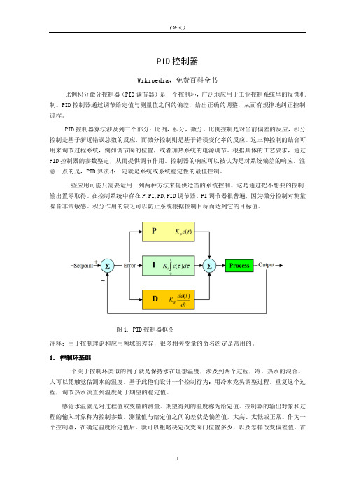
图1. PID控制器框图注释：由于控制理论和应用领域的差异，很多相关变量的命名约定是常用的。

1．控制环基础一个关于控制环类似的例子就是保持水在理想温度，涉及到两个过程，冷、热水的混合。

人可以凭触觉估测水的温度。

基于此他们设计一个控制行为：用冷水龙头调整过程。

重复这个过程，调节热水流直到温度处于期望的稳定值。

感觉水温就是对过程值或变量的测量。

期望得到的温度称为给定值。

控制器的输出对象和过程的输入对象称为控制参数。

测量值与给定值之间的差就是偏差值，太高、太低或正常。

作为一个控制器，在确定温度给定值后，就可以粗略决定改变阀门位置多少，以及怎样改变偏差值。

首次估计即是PID 控制器的比例度的确定。

当它几乎正确时，PID控制器的积分作用就是起着逐渐调整温度的作用。

微分作用就是根据水温变得更热、更冷，以及变化速率来决定什么时候、怎样调整那些阀门。

当偏差小时而做了一个大变动，相当于一个大的调整控制器，会导致超调。

外文资料与翻译PID Contro lIntroductionThe PID controller is the most common form of feedback. It was an essential element of early governors and it became the standard tool when process control emerged in the 1940s. In process control today, more than 95% of the control loops are of PID type, most loops are actually PI control. PID controllers are today found in all areas where control is used. The controllers come in many different forms. There are standalone systems in boxes for one or a few loops, which are manufactured by the hundred thousands yearly. PID control is an important ingredient of a distributed control system. The controllers are also embedded in many special purpose control systems. PID control is often combined with logic, sequential functions, selectors, and simple function blocks to build the complicated automation systems used for energy production, transportation, and manufacturing. Many sophisticated control strategies, such as model predictive control, are also organized hierarchically. PID control is used at the lowest level; the multivariable controller gives the set points to the controllers at the lower level. The PID controller can thus be said to be the “bread and butter of control engineering. It is an important component in every co ntrol engineer’s tool box.PID controllers have survived many changes in technology, from mechanics and pneumatics to microprocessors via electronic tubes, transistors, integrated circuits. The microprocessor has had a dramatic influence the PID controller. Practically all PID controllers made today are based on microprocessors. This has given opportunities to provide additional features like automatic tuning, gain scheduling, and continuous adaptation.6.2 The AlgorithmWe will start by summarizing the key features of the PID controller. The “textbook” version of the PID algorithm is described by:()()()()⎪⎪⎭⎫ ⎝⎛++=⎰dt t de d e t e K t u T T d t i 01ττ 6.1 where y is the measured process variable, r the reference variable, u is the control signal and e is the control error （e =sp y − y ）. The reference variable is often calledthe set point. The control signal is thus a sum of three terms: the P-term （which is proportional to the error）, the I-term （which is proportional to the integral of the error）, and the D-term （which is proportional to the derivative of the error）. The controller parameters are proportional gain K, integral time T i, and derivative time T d. The integral, proportional and derivative part can be interpreted as control actions based on the past, the present and the future as is illustrated in Figure 2.2. The derivative part can also be interpreted as prediction by linear extrapolation as is illustrated in Figure 2.2. The action of the different terms can be illustrated by the following figures which show the response to step changes in the reference value in a typical case.Effects of Proportional, Integral and Derivative ActionProportional control is illustrated in Figure 6.1. The controller is given by D6.1E with T i= and T d=0. The figure shows that there is always a steady state error in proportional control. The error will decrease with increasing gain, but the tendency towards oscillation will also increase.Figure 6.2 illustrates the effects of adding integral. It follows from D6.1E that the strength of integral action increases with decreasing integral time T i. The figure shows that the steady state error disappears when integral action is used. Compare with the discussion of the “magic of integral action” in Sec tion 2.2. The tendency for oscillation also increases with decreasing T i. The properties of derivative action are illustrated in Figure 6.3.Figure 6.3 illustrates the effects of adding derivative action. The parameters K and T i are chosen so that the closed loop system is oscillatory. Damping increases with increasing derivative time, but decreases again when derivative time becomes too large. Recall that derivative action can be interpreted as providing prediction by linear extrapolation over the time T d. Using this interpretation it is easy to understand that derivative action does not help if the prediction time T d is too large. In Figure 6.3 the period of oscillation is about 6 s for the system without derivative Chapter 6. PID ControlFigure 6.1Figure 6.2Derivative actions cease to be effective when T d is larger than a 1 s (one sixth of the period). Also notice that the period of oscillation increases when derivative time is increased.A PerspectiveThere is much more to PID than is revealed by （6.1）. A faithful implementation of the equation will actually not result in a good controller. To obtain a good PID controller it is also necessary to consider。

International Conference on Advances in Mechanical Engineering and Industrial Informatics (AMEII 2015)Design and Implementation of UAV Flight Simulation Based onMatlab/SimulinkZheng Xing1,a, Yang He2,b, Cheng Jian1,c1Wuhan Mechanical Technology College, Wuhan, 430075, China2Hubei University of Education, Wuhan, 430205, Chinaa email:********************,b email:*****************,c email:**************************omKey words: UAV, Simulation Training, Matlab/Simulink, Flight Simulation, Mode SwitchAbstract.This paper elaborates the composition and function of the flight simulation system according to characteristics of UAV flight simulation in simulation training device. Flight control model and navigation model are designed based on the Matlab/Simulink to solve mode switch and other key technical difficulties in software.IntroductionUA V has been one of important weapon equipment in modern wars and has been widely used in civil areas. As the UA V plays a more and more important role, while accelerating R&D and equipping of advanced UA V system, countries worldwide pay more attention to research of training system and methods based on practical requirements in order to enhance UA V application performance. Currently, extensive developments and applications have been conducted for UA V simulation training systems of different types. The first aim is to improve the ability of flight personnel through simulation training. In order to implement real flight control training, a flight simulation environment should be established[1]. When the effect of flight simulation is closer to real UA V flight status, UA V control personnel’s skills will be improved more.Composition of Flight Simulation SystemFlight simulation computer hardware is composed of an IPC which communicates with system equipment via network port or serial port[2].The software platform is based on general-purpose Windows operating system. In order to simulate the real-time control function of a stabilized turntable, Ardence RTX products will be used. This product offers a real-time subsystem on Windows platform to ensure real-time control, tracking and response on Windows platform. Software consists of two parts: flight control model and navigation model.The former performs digital simulation of real devices of aircraft including aerodynamic device, flight-control computer, actuator, vertical gyro, rate gyro and magnetic heading sensor; the latter controls the UA V to fly at the designated flight path.Design and Implementation of Flight SimulationFor flight control model and navigation model, the mathematical simulation method is used to simulate real devices including flight-control computer, navigation computer, aircraft power and aerodynamic systems and actuator.Development tool.Graphical simulation modeling tool and simulation programming language are mainly used for modeling, and it is Matlab/Simulink that represents a combination of them. The modeling and debugging for the whole flight simulation including aircraft model, control law, sensor model and actuator model are implemented by Matlab/Simulink[3]. Aircraft model and sensormodel can be selected from Simulink model library [4]. For the control law module, S function interfaces written in C/C++ language provided by Simulink can be used to implement mixed programming of Simulink and C/C++ language; then the model can be easily modified and debugged by calling S function written in C/C++ language and making good use of Simulink visual modeling capability.Composition and function. The whole simulation model consists of flight control model (which is used to simulate dynamic characteristics of the aircraft) and navigation model. A six-DoF nonlinear model of aircraft is established based on aerodynamic data. The key to sensor model in the flight control model is how to simulate sensor noise accurately. According to physical properties of the sensor, noise signals are superposed at the output end of the sensor to simulate measured signal noise and error. Dead area, saturation and other nonlinear factors often exist in the actuator. So in the model, dead area and saturation parameters are properly set to simulate the actuator.Flight control model. In a real UA V system, the flight control system is an integrated controller responsible for coordinating and managing all subsystems of the UA V , and is also the core of UA V flight management and control. Therefore, the implementation of the flight control module is a basic and key part in UA V flight simulation.Mathematical modeling. To research into UA V flight control, we first have to establish a model for the research object. In modeling, the following assumptions are always made: the Earth is the inertial reference system; the aircraft is a rigid body; the weight is a constant; and acceleration of gravity does not change with flight altitude. By reference to airframe coordinates, six dynamic differential equations are established to describe the movement of aircraft.[5] The said equations are complex in structure, so they are only suitable for numeric calculation. For the convenience of controller design, a small-disturbance linearized method can be used to obtain the small-disturbance linear state equation of UA V at the equilibrium point.[6] Furthermore, the aircraft is symmetrical, so linear results are divided into two groups, which describe longitudinal movement and lateral movement, respectively. Therefore, five control modes are established for flight control model, including elevation holding and control, altitude holding and control, roll angle holding and control, course angle holding and control, lateral deviation control.The longitudinal small-disturbance linear equation of UA V with wind disturbance is: [7] X AX BU Fd =++where, 100001000010T F = ; 000x y zW V W U d q W x α−∆==∆∆∂∂ ; U 0 is airspeed component along the vertical axis;W x , W y and W z are three components for wind speed; X = [ΔV Δα q Δθ]T ; U = δe .The lateral small-disturbance linear equation of UA V with wind disturbance is: X AX BU Fd =++ where, 100001000010T F= ; 00z y x W U W z d p r W z β∆∂∂==∆∆∂∂ ; U 0 is airspeed component along the vertical axis; W x , W y and W z are three components for wind speed; []T X p βψγ= ; []T a r U δδ=.Design of control law. PID controller is used for the module. The system is under error-based negative feedback control. The controller takes the difference between system output feedback quantity and an expected value or a set value as the input quantity, and with an algorithm, obtains a control quantity to make the output quantity change with the input quantity.[8]Take the design of longitudinal pitch channel of aircraft as an example. The pitch angle and pitch rate feedback are used for pitch attitude holding and control of the aircraft. Pitch rate feedback is realized by the angular rate compensator and the pitch angle is measured by the sensor. The throttle opening is temporarily deemed to be constant, and is not taken into account. Then, the pitch channelcontrol model is designed with Simulink tool kit in Matlab.Navigation model. The navigation system is an integral part of the UA V system. It is capable of providing support for tactical operations of the UA V through satellite navigation, AWACS guiding, ground guiding and UA V capability of detecting and tracking targets. It is mainly used to implement real-time location and automatic control of flight path of the UA V.UA V’s navigation function is based on the coordinated turn function.[9]First, the system determines the current course of an aircraft according to voyage points, measures and calculates the lateral deviation distance between aircraft and flight path, track deviation angle and current ground velocity of aircraft in real time, and then solves a lateral driving signal in accordance with the navigation control law, and gives a bank angle to control the aircraft to enter coordinated turn, and when both lateral deviation distance and track deviation angle are zero, the aircraft performs a straight and level flight along the current flight course until it enters the next point.The simulation of navigation control law is based on flight control law simulation. The navigation control law is designed by integrating each separate channel into full dimension simulation and taking cross track distance and yaw angle as input values.Implementation of Simulation Technology DifficultiesThe flight simulation system is very close to a real system, but different from the real system. In simulation training, UA V is required to perform some extreme actions and random switch among modes, and humanity principle shall be followed during the training. This leads to considerable difficulty and many logical problems in programming. The whole module is of purely digital analog, so mode switch in real-time module may involve problems about zero clearing of many integral terms. In case of failure in timely zero clearing, accumulated values will affect the whole flight simulation result, and even cause systematic divergence, so that the control law could not be successfully implemented. Mutual independence of longitudinal channel and lateral channel is used. When receiving a command about changing longitudinal movement, the system only clears integral terms under longitudinal control, and integral terms under lateral control will keep accumulating until a command about changing lateral movement is received. Zero clearing of lateral integral terms is performed in a similar way.Abovementioned processes will both satisfy requirements of practical simulation training and show simulative extreme action simulation, thereby training operator’s emergency response capability.ConclusionThe flight simulation design of the simulation training device is implemented in the abovementioned method. According to the simulation result, control of modes of the aircraft meets specification requirements, the transition process during switch among modes is stable and the flight profile trend coincides. The design model can truly simulate UA V flight control and navigation and implement real-time simulation of pre-flight preparation, launch, cruising, program-control, manual control, mode switch and recovery controlled by the ground console. It has high confidence level and reliability in simulation, strong expandability and wide application. AcknowledgementThis work is supported by the natural science foundation of Hubei Province No.2014CFB569. This work is also supported by the research project of Hubei Province Department of Education Grant No.Q20133008.References[1] Peng Hua, Shen Weiqun, Song Zishan, A Real-time Management System of Flight SimulationBased on VxWorks, Journal of System Simulation, 2003, 15(7): 966-968.[2] Zhang Ning, Chen Ning, Ji Yun, Zhu Jiang, Research on The Integrated Method of FlightSimulation System Based on A Flight Simulator, Flight Dynamics, 2010, 28(3): 39-42.[3] Zhang Lei, Jiang Hongzhou, Qi Panguo, Li Hongren, Flight Simulation Based on Matlab,Computer Simulation, 2006, 23(6): 57-61.[4] Shang Wenxuan, Wang He, Gao Ya, The Avionic System Platform Based on Flight Simulationof Simulink and Its Application, Electronics Optics & Control, 2014, 21(8): 6-9.[5] Zhang Minglian, Flight Control System, National Defense Industry Press, 1993.[6] Xu Hailiang, Li Junyang, Fei Shumin, Design and Implementation of Digital Flight SimulationPlatform, Journal of Southeast University(Natural Science Edition), 2011, 41(1): 113-117. [7] Su Jijie, Zheng Xing, Lin Dongsheng, Yang Yi, Design and Implementation of SimulativeTraining System for UAV, Journal of System Simulation, 2009, 21(5): 1343-1346.[8] Li Chao, Wang Jiangyun, Han Liang, Development of Fixed Wing Aircraft Flight SimulationSystem Based on Matlab, Journal of System Simulation, 2013, 25(8).[9] Gen Tongfen, Huang Daqing, Full Process Simulation of UAV Auto-pilot Flight Based onSimulink, Aeronautical Computing Technique, 2010, 40(5): 112-116.。

模型不确定二质量系统的振动抑制与实验研究徐宝申;周波【摘要】针对电机柔性连接负载驱动系统在加减速时会产生不稳定的扭转振动,以及刚度系数测量复杂且难以准确计算的问题,提出了通过对开环系统电机端速度响应进行时频分析,识别系统谐振频率以及调整时间的方法,进而设计了一种IP反馈控制与输入整形前馈相结合的振动抑制控制器,在提高系统响应速度的同时,达到较好的振动抑制效果.在模型不确定二质量扭转谐振平台上进行实验研究,实验结果表明该方法能够有效抑制负载端振动,并显著提高系统响应速度.【期刊名称】《实验技术与管理》【年(卷),期】2019(036)003【总页数】4页(P175-178)【关键词】振动抑制;二质量扭转系统;模型不确定;时频分析;IP控制器【作者】徐宝申;周波【作者单位】北京城市学院资源设备管理办公室 ,北京 101309;北京城市学院信息学部 ,北京 101309【正文语种】中文【中图分类】TP273工业生产设备中普遍存在柔性连接负载,使伺服系统在加减速过程中产生振动,不但严重影响设备安全运行,而且迫使伺服系统降低响应速度,以致影响伺服系统的控制品质。

电机驱动系统通常可视为二质量柔性扭转系统,研究此类柔性负载的振动抑制问题对提高伺服系统性能具有重要意义[1]。

针对二质量系统振动抑制的研究成果包括基于多项式惯量比的低阶IP控制器设计[2]、基于极点配置的PI/PID控制器设计[3-4]、模糊控制及神经网络控制[5-6]等。

其中采用低阶IP控制的方法结构简单、参数设计方便,在工业中得以广泛采用。

此外,为进一步提高系统响应速度,研究人员引入输入整形前馈以实现机构残余振动的快速抑制[7]。

然而,不论是输入整形器还是低阶IP控制器,均依赖系统的模型参数。

但在实际工程应用中,难以对柔性轴的刚度系数和系统谐振频率精确建模。

此外,生产现场伺服系统只有电机端速度可测,而由于传动间隙及减速比等原因,电机端速度振动微小,传统分析手段很难识别出系统的特征参数。

DPST-8000M Pitot Static Test Set“Exceeds RVSM High Accuracy Standards”Cage Code # 3PTA2General InformationT he Model DPST-8000 Pitot Static Test Set is a precision test set with dual channel pressure controller, designed to provide regulated total (PT) pressure and static (PS) pressure outputs to simulate Altitude, Airspeed and Vertical Speed param-eters. The test set can also be used in a laboratory environ-ments to calibrate Altimeters, Airspeeds and ADC’s in maintenance shops or in harsh hangar environments. The test set is compact, light weight and has aremovable storage lid, which can fit in theoverhead compartmenton a commercialairliner.• Ports have self sealing quick connections, which are color coated and keyed to protect the aircraft and test equipment from pressure loss or incorrect system connections.• Internal pumps produce pressure and vacuum, which fill holding tanks for quick start ups and high performance rates. Exceeds 60,000 ft. of altitude, 15,000 ft./min VSI rate and 650 knots of airspeed.• Certified to perform Reduced Vertical Separations Minimum on fixed or rotary wing aircrafts.• Precision microprocessor based with Honeywell sensors, accuracy to 0.001% of full range.• Sun-light readable color TFT display showing real instrument EFD presentation.•The simple pop-up screens display the Altitude, Vertical Speed, Airspeed EPR and other measurements in various units of measure, including Ft, M, Kts, Km/hr, Mach, Ft/min, M/min, EPR (Pt/Ps), inHg, mb and psia. All readings are up-dated every 2 tenths of a second.• Automatic pitot and static leak rate modes automatically perform calculations & system failures.•Precision metering valves with protection shut off seats for maximum control rates.Standard Features Dimensions 20”L x 16”W x 8”H 25 lbs.• Water resistance and temperature corrected for extreme flightline conditions.• Smart AC power supply for safe flight line usage input voltages 85 to 264 V AC / 47 to 440 Hz• Storm Case constructed meets all applicable requirements of MIL-STD-810 removable lid, with fixed storage bag and watertight standards to MIL-108.• Test set is equipped with quick connect fittings and 2 hoses thatare each 20 ft in length.•Calibration meets or exceeds the published specifications,which are traceable to the National Institute Standards andTechnology “N.I.S.T.”.To buy, sell, rent or trade-in this product please click on the link below:/DFW-Instruments-DPST-8000M-Manual-Digital-RVSM-Air-Data-Test-Set.aspxDigital Manual RVSM Pitot Static Test Set DPST-8000M Performance SpecificationsAbsolute Pressure PerformanceStatic Pressure:Range: 0.3 to 40 inHg abs.Accuracy: +/- 0.001 inHg FS Repeatability: +/- 0.0008 inHgDrift: +/- 0.004 inHg per year FS Overpressure: 300 % FS without damagePitot Pressure:Range: 0.8 to 80 inHg abs.Accuracy: +/- 0.001 inHg FS Repeatability: +/- 0.002 +/- 100 ppm/yearDrift: +/- 0.01 inHg per year max. Overpressure: 300 % FS without damage Altitude PerformanceRange: -2000 ft. to 55,000 ft. Resolution: 1 ft.Accuracy: ±2 ft. @ 0 ft.±5 ft. @ 35,000 ft.±12 ft. @ 55,000 ft.Rate of Climb PerformanceRange: 100 ft./min. to 20,000 ft./min. Resolution: 1 ft./min.Accuracy: ±1 % of rate with a min. of 10 ft./min. Airspeed PerformanceRange: 10 to 600 KnotsResolution: 0.5 KnotsAccuracy: ±0.5 Knots@ 20 knots±0.05 Knots @ 600 knotsMach PerformanceRange: 0.0 Mach to 5.0 Mach Resolution: 0.001 MachAccuracy: 0.01 Mach above 0.1 Machfor Ps = 29.921 InHg.EPR PerformanceRange: 0.1 to 3.0 (Ps @ 30inHg) Resolution: 0.001Accuracy: 0.05 %FS PSI Pressure MediumDry AirPressure ConnectionsQuick Disconnects (2 ea.)Safety Seal on Female Quick ConnectDisplay Update RateOnce Every 2 Tenths per SecondOutputsUSB Port / Data Output / RS-485 (Additional Fees) SensorsHoneywell Certified Sensors (NIST Traceable)Power RequirementInput Range: 85 - 264 V ACFrequency Range: 47 Thru 440 Hz Environmental SpecsTemp. Operating: 0° C to +50° CTemp. Storage: -25° C to +60° C Humidity: 0% to 95% RH20 Warranty & CalibrationWarranty: 2 years (parts & labor) Calibration: Up to 1 year (yearly calibration suggested) RVSM CertificationCalibration / Trace to NISTExceed RVSM Accuracy Compliance Specs Physical Dimensions20” L x 15” W x 7“H Mil-STD810FWeight Case23 Lbs. Storm CaseORDERING INFORMATIONMfg. Part Number: DPST-8000M Accessories Include: Protection Quick Release Fittings, Hoses, Shipping Container and Operation Manual.。