Weibull_Reliability_Analysis 威布尔分布(韦伯分布)可靠性分析
- 格式:xlsx
- 大小:37.26 KB
- 文档页数:1
Weibull分布(韦伯分布)(2006-07-04 22:04:01)转载分类:学习Weibull分布,又称韦伯分布、韦氏分布或威布尔分布,由瑞典物理学家Wallodi Weibull于1939年引进,是可靠性分析及寿命检验的理论基础。
Weibull分布能被应用于很多形式,包括1参数、2参数、3参数或混合Weibull。
3参数的该分布由形状、尺度(范围)和位置三个参数决定。
其中形状参数是最重要的参数,决定分布密度曲线的基本形状,尺度参数起放大或缩小曲线的作用,但不影响分布的形状。
另外,通过改变形状参数可以表示不同阶段的失效情况;也可以作为许多其他分布的近似,如,可将形状参数设为合适的值近似正态、对数正态、指数等分布。
形状参数通常在[1,7]间取值。
一般由W(α,β)表示2个参数的Weibull分布,其分布函数为:,其中x>0,α、β>0。
可以看出有两个参数α、β,其中β为形状参数,α为尺度参数。
若取β为1,则F(x)为指数分布。
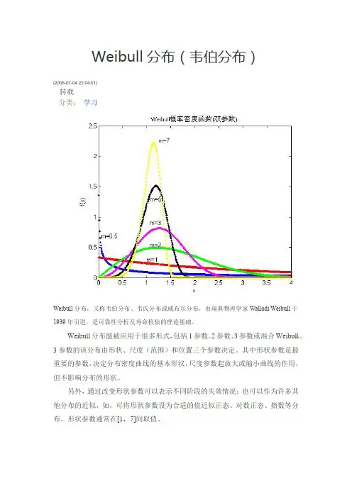
Weibull分布的概率密度函数(pdf)为:。
Weibull双参数的PDF分布见上图。
(自己做的,有点粗糙)下面我们以其pdf图看Weibull分布各参数的作用。
下图是形状参数β对pdf的影响(α固定):下图为尺度参数α对pdf的影响(β固定),横轴为变量x,纵轴为f(x):另外,由于Weibull分布可以近似表示其他别的分布,eg,β=1时,F(x)为指数分布。
将其用到复杂网络中,则此时对应指数网络?当β逐渐增大时,是不是对应分布极不均匀的无尺度网络?这样的话可以通过调整一个参数构造不同的网络?而**人的层次故障节点动态模型就是因此而引入Weibull分布(1参数)的吧?这样的话,β大的网络发生层次故障的规模比较大就可以理解了。
再继续深入分析。


六西格玛培训—验证阶段模块可靠性分析Patrick ZhaoI&CIM Deployment Champion可靠性分析介绍执行可靠性分析可靠性分析介绍执行可靠性分析可靠性与质量•狭义的质量,一般指的是符合性质量,即是否满足标准或规范,通常是以产品出厂时的状态为准,此时传统的质量控制人员已经完成任务。
•可靠性更多关注在产品的全生命周期中的质量表现,即产品是否能够始终满足标准,始终满足客户的应用。
在如今全面质量管理的阶段,产品的可靠性也越来越需要企业投入更多的时间。
•企业中的可靠性分析可以分为产品和过程:•产品:分析产品在客户使用中是否满足可靠性目标。
•过程:一般指设备、工装、模具等在长期使用过程中,是否会出现问题。
可靠性工程的益处•在物质匮乏的年代,衣服可能是作为耐用品使用,而如今衣服已经越来越成为快速消费品。
曾经的手机等电子产品,更换周期也同样有越来越短的趋势。
甚至是汽车也开始加速迭代,不停缩短换车的时间。
•在这样的背景下,可靠性似乎成为了一个不是那么重要的关注点,可是为什么我们仍然在关注可靠性工程?•政府、法规的要求。
•不可靠的产品通常有安全或健康风险。
•产品变得复杂,零件变多,更容易发生故障。
•可靠性的优势可以成为销售和市场部门的宣传点。
•处于保护环境,节约资源的考虑。
可靠性分析的常用术语•浴缸曲线(Bathtub Curve)•MTTF: Mean Time To Failure(平均失效前时间)•MTTR: Mean Time To Repair(平均修复时间)•MTBF: Mean Time Between Failure(平均故障发生间隔时间)•威布尔分布(Weibull Distribution)•数据删失(Data Censoring)•HALT: Highly Accelerated Life Testing(高加速寿命试验)•HASS: Highly Accelerated Stress Screening(高加速应力筛选)•HASA: Highly Accelerated Stress Audit(高加速应力稽核/抽检)浴缸曲线•浴缸曲线(Bathtub Curve)在可靠性分析中是一种常用的概念,它把失效分为三个阶段。

基于非线性最小二乘法的威布尔分布参数估计摘要:针对传统威布尔参数估计方法对于初值要求较高且精度不高的问题,提出了非线性最小二乘法参数估计算法。
首先介绍三参数威布尔分布的函数形式;然后阐述了非线性最小二乘法的基本原理;最后采用某机构液压锁寿命数据作为算例验证本文方法,算例表明基于最小二乘法的威布尔分布参数估计精度较高,具有一定的工程应用价值。
关键字:威布尔分布非线性最小二乘法参数估计前言瑞典科学家W.Weibull根据两参数威布尔分布构建了而三参数威布尔(Weibull)分布。
在估计三参数Weibull分布参数时,现在最常用的方法包括图解法、极大似然法、最小二乘法、线性回归估计法等[3]。
其中,图解法操作简单,但估计值精度不高;后三种解析法在样本量较大时,其估计效果较好,但在当拟合的函数为非线性函数时,估计精度将大为下降,从而使得这三种算法面对非线性函数拟合时失去应用价值。
为此本文引进非线性最小二乘算法。
非线性最小二乘算法非常适合解决非线性函数的参数估计问题。
非线性最小二乘法通过特定的变换方法,将非线性问题转换为线性问题;再得到线性函数估计值后,再根据转换关系式将其转换为非线性函数的估计值。
以某机构液压锁寿命为算例,结果表明非线性最小二乘法参数估计精度较高,具有一定的工程应用价值。
1威布尔分布简介三参数Weibull分布是一种比较完善的分布,在拟合随机数据方面十分灵活,适应性很强。
因此,三参数Weibull分布能更准确地描述疲劳寿命的概率分布,而且,在可靠性研究领域中的几种常用分布,如指数分布、瑞利分布等都可看作是三参数Weibull分布的特例。
若随机变量X服从三参数威布尔分布,则其概率密度函数为:其中,为Gamma函数。
2 非线性最小二乘法当模型中拟合参数与被拟合数据之间呈现为非线性函数关系时,就形成非线性拟合。
非线性拟合较难处理,有时甚至连解的存在性和唯一性都难以确定。
有些非线性拟合,在通过对拟合参数或/和原始数据的适当函数变换后,能使“变换后拟合参数”与“变换后原始数据”之间的关系呈现为线性形式;则称这种非线性拟合是“非本质的非线性”;而这种变换处理方式称为“伪线性化”。


招聘可靠度工程师笔试题与参考答案(某世界500强集团)(答案在后面)一、单项选择题(本大题有10小题,每小题2分,共20分)1、可靠度工程师在进行产品寿命预测时,通常使用以下哪种方法?A、蒙特卡洛模拟B、线性回归分析C、时间序列分析D、神经网络分析2、在可靠性试验中,以下哪个参数是用来描述产品失效时间的?A、平均故障间隔时间(MTBF)B、平均修复时间(MTTR)C、故障率(FR)D、失效率(λ)3、在可靠性工程中,以下哪个指标可以用来评估产品在特定时间内发生故障的概率?A. 平均无故障时间(MTBF)B. 平均故障间隔时间(MTTF)C. 失效率(λ)D. 平均修复时间(MTTR)4、以下哪个选项是可靠性增长的典型曲线?A. S形曲线B. 对数正态分布曲线C. 贝塔分布曲线D. 指数分布曲线5、在可靠性工程中,以下哪个指标是用来衡量产品在规定时间内,完成规定功能的概率?A. 平均无故障时间(MTBF)B. 可靠度(R(t))C. 失效率(λ)D. 浴盆曲线6、以下哪种方法常用于评估产品的可靠性设计是否满足要求?A. 故障树分析(FTA)B. 有限元分析(FEA)C. 质量控制图(QC图)D. 六西格玛分析7、在可靠性工程中,MTBF(平均故障间隔时间)指的是什么?A. 设备从首次使用到发生第一次故障的时间B. 设备在两次连续故障之间的平均运行时间C. 设备修复并重新投入使用的时间D. 设备完全失效后不再修复的时间8、在进行可靠性分析时,哪种分布常用于描述电子产品或机械产品的故障率?A. 正态分布B. 泊松分布C. 指数分布D. 威布尔分布9、在软件可靠度评估中,以下哪个指标通常用于衡量系统在特定时间内发生故障的概率?()A、可靠性增长率B、平均故障间隔时间(MTBF)C、故障率D、平均修复时间(MTTR) 10、在软件可靠性增长模型中,以下哪个模型假设软件缺陷的分布是指数分布的?()A、Weibull模型B、泊松模型C、Gamma模型D、Lognormal模型二、多项选择题(本大题有10小题,每小题4分,共40分)1、以下哪些因素会影响可靠度工程师在评估产品可靠性时所采用的故障模式与影响分析(FMEA)的准确性?()A、故障模式识别的全面性B、故障原因分析的正确性C、潜在影响评估的准确性D、预防措施的有效性E、风险评估的客观性2、在可靠性设计中,以下哪些方法可以提高产品的可靠性?()A、冗余设计B、热设计C、故障安全设计D、环境适应性设计E、标准化设计3、在可靠性工程中,故障模式及影响分析(FMEA)的主要目的是什么?(多选)A. 分析系统可能的故障模式B. 确定每个故障模式对系统的影响C. 提供一种方法来降低产品成本D. 评估现有控制措施的有效性E. 识别并优先处理潜在的设计缺陷4、关于可靠性指标MTBF(平均无故障时间)和MTTR(平均修复时间),下列说法哪些是正确的?(多选)A. MTBF是指设备从一次故障恢复到下一次故障发生的时间间隔B. 较高的MTBF值意味着更好的系统可靠性C. MTTR指的是从故障发生到完全恢复正常运行所需的时间D. 较低的MTTR值表示更快速有效的维护响应E. 在评估系统可靠性时,仅考虑MTBF而不考虑MTTR是充分的5、以下哪些是可靠度工程师在工作中需要掌握的软件工具?()A. MATLABB. SPSSC. ANSYSD. SolidWorksE. Excel6、以下关于可靠性试验的说法,正确的是?()A. 可靠性试验分为环境应力筛选试验和寿命试验B. 环境应力筛选试验的目的是检测产品在特定环境下的可靠性C. 寿命试验的目的是确定产品的失效寿命分布D. 可靠性试验通常需要在实验室进行E. 可靠性试验结果可以用于制定产品的质量标准7、以下哪些因素会影响可靠度工程师在产品寿命周期内的任务重点?()A. 产品设计阶段B. 产品制造阶段C. 产品使用阶段D. 产品维护阶段E. 产品回收阶段8、以下关于可靠性试验的描述,正确的是哪些?()A. 可靠性试验是评估产品可靠性的主要方法之一。
威布尔分布如何根据形状参数,尺度参数,截距等拟合公
式
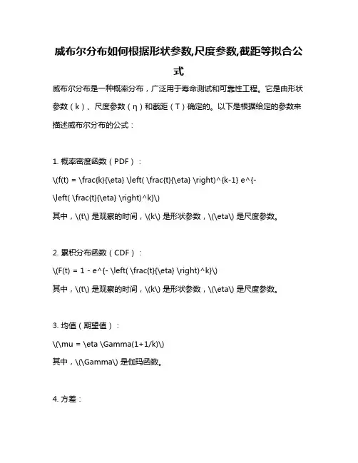
威布尔分布是一种概率分布,广泛用于寿命测试和可靠性工程。
它是由形状参数(k)、尺度参数(η)和截距(T)确定的。
以下是根据给定的参数来描述威布尔分布的公式:
1. 概率密度函数(PDF):
\(f(t) = \frac{k}{\eta} \left( \frac{t}{\eta} \right)^{k-1} e^{-
\left( \frac{t}{\eta} \right)^k}\)
其中,\(t\) 是观察的时间,\(k\) 是形状参数,\(\eta\) 是尺度参数。
2. 累积分布函数(CDF):
\(F(t) = 1 - e^{- \left( \frac{t}{\eta} \right)^k}\)
其中,\(t\) 是观察的时间,\(k\) 是形状参数,\(\eta\) 是尺度参数。
3. 均值(期望值):
\(\mu = \eta \Gamma(1+1/k)\)
其中,\(\Gamma\) 是伽玛函数。
4. 方差:
\(\sigma^2 = \eta^2 \left[ \Gamma(1+2/k) - \Gamma^2(1+1/k)
\right]\)
其中,\(\Gamma\) 是伽玛函数。
这些公式可以根据给定的参数(形状参数、尺度参数和截距)进行拟合。
在实践中,通常会使用最大似然估计法(MLE)或其它统计方法来估计这些参数。

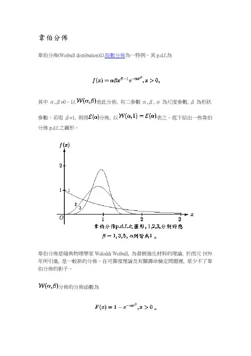
韋伯分佈韋伯分佈(Weibull distribution)以指數分佈為一特例。
其p.d.f.為其中α,β>0。
以表此分佈, 有二參數α,β, α為尺度參數, β為形狀參數。
若取β=1, 則得分佈, 以表之。
底下給出一些韋伯分佈p.d.f.之圖形。
韋伯分佈是瑞典物理學家Waloddi Weibull, 為發展強化材料的理論, 於西元1939年所引進, 是一較新的分佈。
在可靠度理論及有關壽命檢定問題裡, 常少不了韋伯分佈的影子。
分佈的分佈函數為期望值與變異數分別為Characteristic Effects of the Shape Parameter, β, for the Weibull DistributionThe Weibull shape parameter, β, is also known as the slope. This is because the value of β is equal to the slope of the regressed line in a probability plot. Different values of the shape parameter can have marked effects on the behavior of the distribution. In fact, some values of the shape parameter will cause the distribution equations to reduce to those of other distributions. For example, when β = 1, the pdf of the three-parameter Weibull reduces to that of the two-parameter exponential distribution or:where failure rate.The parameter β is a pure number, i.e. it is dimensionless.The Effect of β on the pdfFigure 6-1 shows the effect of different values of the shape parameter, β, on the shape of the pdf. One can see that the shape of the pdf can take on a variety of forms based on the value of β.Figure 6-1: The effect of the Weibull shape parameter on the pdf.For 0 < β1:∙As (or γ),∙As , .∙f(T) decreases monotonically and is convex as T increases beyond the value of γ.∙The mode is non-existent.For β > 1:∙f(T) = 0 at T = 0 (or γ).∙f(T) increases as (the mode) and decreases thereafter.∙For β < 2.6 the Weibull pdf is positively skewed (has a right tail), for 2.6 < β < 3.7 its coefficient of skewness approaches zero (no tail). Consequently, it may approximatethe normal pdf, and for β > 3.7 it is negatively skewed (left tail).The way the value of β relates to the physical behavior of the items being modeled becomes more apparent when we observe how its different values affect the reliability and f ailure ratefunctions. Note that for β = 0.999, f(0) = , but for β = 1.001, f(0) = 0. This abrupt shift is what complicates MLE estimation when β is close to one.The Effect ofβ on the cdf and Reliability FunctionFigure 6-2: Effect of β on the cdf on a Weibull probability plot with a fixed value of η.Figure 6-2 shows the effect of the value of β on the cdf, as manifested in the Weibull probability plot. It is easy to see why this parameter is sometimes referred to as the slope. Note that the models represented by the three lines all have the same value of η. Figure 6-3 shows the effects of these varied values of β on the reliability plot, which is a linear analog of the probability plot.Figure 6-3: The effect of values of β on the Weibull reliability plot.∙R(T) decreases sharply and monotonically for 0 < β < 1 and is convex.∙For β = 1, R(T) decreases monotonically but less sharply than for 0 < β < 1 and is convex.∙For β > 1, R(T) decreases as T increases. As wear-out sets in, the curve goes through an inflection point and decreases sharply.The Effect of β on the Weibull Failure Rate FunctionThe value of β has a marked effect on the failure rate of the Weibull distribution and inferences can be drawn about a population's failure characteristics just by considering whether the value of β is less than, equal to, or greater than one.Figure 6-4: The effect of β on the Weibull failure rate function.As indicated by Figure 6-4, populations with β < 1 exhibit a failure rate that decreases with time, populations with β = 1 have a constant failure rate (consistent with the exponential distribution)and populations with β > 1 have a failure rate that increases with time. All three life stages of the bathtub curve can be modeled with the Weibull distribution and varying values of β.The Weibull failure rate for 0 < β < 1 is unbounded at T = 0 (or γ). The failure rate, λ(T), decreases thereafter monotonically and is convex, approaching the value of zero asor λ( ) = 0. This behavior makes it suitable for representing the failure rate of units exhibiting early-type failures, for which the failure rate decreases with age.When encountering such behavior in a manufactured product, it may be indicative of problems in the production process, inadequate burn-in, substandard parts and components, or problems with packaging and shipping.For β = 1, λ(T) yields a constant value of or:This makes it suitable for representing the failure rate of chance-type failures and the useful life period failure rate of units.For β > 1, λ(T) increases as T increases and becomes suitable for representing the failure rate of units exhibiting wear-out type failures. For 1 < β < 2, the λ(T) curve is concave, consequently the failure rate increases at a decreasing rate as T increases.For β = 2 there emerges a straight line relationship between λ(T) and T, starting at a value ofλ(T) = 0 at T = γ, and increasing thereafter with a slope of . Consequently, the failurerate increases at a constant rate as T increases. Furthermore, if η = 1 the slope becomes equal to 2, and when γ = 0, λ(T) becomes a straight line which passes through the origin with a slope of 2. Note that at β = 2, the Weibull distribution equations reduce to that of the Rayleigh distribution.When β > 2, the λ(T) curve is convex, with its slope increasing as T increases. Consequently, the failure rate increases at an increasing rate as T increases indicating wear-out life.TopCharacteristic Effects of the Scale Parameter, η, for the Weibull DistributionFigure 6-5: The effects of η on the Weibull pdf for a common β.A change in the scale parameter η has the same effect on the distribution as a change of the abscissa scale. Increasing the value of η while holding β constant has the effect of stretching out the pdf. Since the area under a pdf curve is a constant value of one, the "peak" of the pdf curve will also decrease with the increase of η, as indicated in Figure 6-5.∙If η is increased while β and γ are kept the same, the distribution gets stretched out to the right and its height decreases, while maintaining its shape and location.∙If η is decreased while β and γ are kept the same, the distribution gets pushed in towards the left (i.e. towards its beginning or towards 0 or γ), and its height increases.η has the same units as T, such as hours, miles, cycles, actuations, etc.TopCharacteristic Effects of the Location Parameter, γ, for the Weibull DistributionThe location parameter, γ, as the name implies, locates the distribution along the abscissa. Changing the value of γ has the effect of "sliding" the distribution and its associated function either to the right (if γ > 0) or to the left (if γ < 0).Figure 6-6: The effect of a positive location parameter, γ, on the position of the Weibullpdf.∙When γ = 0, the distribution starts at T = 0 or at the origin.∙If γ > 0, the distribution starts at the location γ to the right of the origin.∙If γ < 0, the distribution starts at the location γ to the left of the origin.∙γ provides an estimate of the earliest time-to-failure of such units.∙The life period 0 to +γ is a failure free operating period of such units.∙The parameter γ may assume all values and provides an estimate of the earliest timea failure may be observed. A negative γ may indicate that failures have occurred priorto the beginning of the test, namely during production, in storage, in transit, duringcheckout prior to the start of a mission, or prior to actual use.∙γ has the same units as T, such as hours, miles, cycles, actuations, etc.。
基于Weibull分布计算在造船设备故障发生概率统计中的应用摘要:造船设备故障发生过程大多遵循一定的客观规律,所以,利用Weibull分布计算对造船设备故障发生概率进行统计,可为造船设备保养与维修提供有效的参考依据。
因此,利用Weibull分布计算,针对造船设备故障的发生规律进行分析,可对设备的可靠度以及故障率等进行计算,对造船设备的维修管理水平提升有促进作用。
关键词:Weibull分布计算;造船设备;故障;概率统计引言:造船设备故障维修包含预防性维修以及故障后维修两种方式,在对造船设备故障进行分析维修过程中,要针对造船设备不同故障的发生概率进行统计与分析,这对保证造船设备的实际应用水平方面有促进作用。
在利用Weibull分布计算的视角下,造船设备故障发生概率统计与分析,以浙江舟山启明电力集团公司的造船设备为研究对象,针对造船生产过程中的关键设备故障发生概率进行统计,对保障生产有现实意义[1]。
1Weibull分布计算逻辑分析Weibull分布计算又名威布尔分布计算,可通过浴盆失效概率曲线的各个阶段对不同故障发生概率进行统计,可提高故障概率分析的准确性及有效性[2]。
设备某一局部失效或者局部故障导致设备停运可服从Weibull分布。
在进行Weibull分布计算中,故障发生概率计算公式如下:在上述公式中,β为形状参数,为尺度参数,β<1,则属于设备的早期故障,β>1则属于耗损故障,β=1为偶发故障。
在对可靠度进行计算与分析中,表示固定条件下,固定时间内完成规定的发生概率。
故障率则是在时间t与t时间点之前发生的概率,可通过可靠度以及故障率的计算,对造船设备发生故障的概率进行统计与分析,为设备故障维修及管理等提供参考依据[3]。
2Weibull分布计算在造船设备故障发生概率统计中的应用2.1案例分析结合浙江舟山启明电力集团公司造船设备故障类型,对不同故障发生概率进行统计与分析。
根据造船设备维修台账,对设备正常运行时间、设备维修时间的分布进行统计与分析。
10分布参数体系分布参数体系是概率统计学中的一个重要概念,用于描述随机变量的分布情况。
它包括了多种常见的概率分布,每个分布都有自己的参数来描述它的特征。
下面我将介绍十种常见的分布参数体系。
1. 正态分布(Normal distribution)是最常见的分布之一,它的参数是均值μ和标准差σ。
正态分布是一个对称的钟形曲线,大部分数据点集中在均值附近,标准差越小,曲线越窄。
2. 二项分布(Binomial distribution)描述了重复n次的独立的二元试验中成功的次数。
它的参数是试验次数n和成功的概率p。
4. 几何分布(Geometric distribution)描述了在一系列独立的伯努利试验直到首次成功之间所需的试验次数。
它的参数是成功的概率p。
5. 负二项分布(Negative binomial distribution)描述了在一系列独立的伯努利试验中直到r次成功所需的试验次数。
它的参数是成功的概率p和成功的次数r。
6. 均匀分布(Uniform distribution)描述了一个随机变量在一个有限的区间上取值的概率是相等的。
它的参数是最小值a和最大值b。
9. 威布尔分布(Weibull distribution)是一种常用的可靠性分布,用于描述时间到达或设备故障的概率。
它的参数是形状参数k和尺度参数λ。
10. 贝塔分布(Beta distribution)是用于描述在一个有限区间内的概率分布,例如概率或比例。
它的参数是两个形状参数α和β。
这些分布参数体系是概率统计学中最常见的分布,它们在不同领域的数据分析和建模中发挥了重要的作用。
通过确定合适的参数值,我们可以根据这些分布来描述和预测随机变量的行为。
这对于决策和风险评估非常重要。
Weibull分布(韦伯分布、威布尔分布)
log函数
从概率论和统计学⾓度看,Weibull Distribution是连续性的概率分布,其概率密度为:
其中,x是随机变量,λ>0是⽐例参数(scale parameter),k>0是形状参数(shape parameter)。
显然,它的累积分布函数是扩展的指数分布函数,⽽且,Weibull distribution与很多分布都有关系。
如,当k=1,它是指数分布;k=2时,是Rayleigh distribution(瑞利分布)。
Weibull概率密度函数
k <1的值表⽰故障率随时间减⼩。
如果存在显着的“婴⼉死亡率”或有缺陷的物品早期失效,并且随着缺陷物品被除去群体,故障率随时间降低,则发⽣这种情况。
在创新扩散的背景下,这意味着负⾯的⼝碑:危险功能是采⽤者⽐例的单调递减函数;
k = 1的值表⽰故障率随时间是恒定的。
这可能表明随机外部事件正在导致死亡或失败。
威布尔分布减⼩到指数分布;
k> 1的值表⽰故障率随时间增加。
如果存在“⽼化”过程,或者随着时间的推移更可能失败的部分,就会发⽣这种情况。
在创新扩散的背景下,这意味着积极的⼝碑:危险功能是采⽤者⽐例的单调递增函数。
该函数⾸先是凹的,然后是凸的,拐点为
Weibull累计分布函数。