复旦大学 研究生投资学讲义 CHPT14- The CAPM ---test
- 格式:pdf
- 大小:61.96 KB
- 文档页数:18


复旦大学经济学院2013~2014学年第二学期期末考试试卷A卷答案(共4页)课程名称:投资学原理课程代码: ECON130031.01开课院系:经济学院考试形式:闭卷姓名:学号:专业:一、选择题(单选或多选:4’*5=20’)1、B2、A C3、B D4、ABD5、CDF二、名词(4’*5=20’)1、股权风险溢价股权风险溢价ERP(equity risk premium,ERP)是指市场投资组合或具有市场平均风险的股票收益率与无风险收益率的差额。
从这个定义可看出:一是市场平均股票收益率是投资者在市场参与投资活动的预期“门槛”,若当期收益率低于平均收益时,理性投资者会放弃它而选择更高收益的投资;二是市场平均收益率是一种事前的预期收益率,这意味着事前预期与事后值之间可能存在差异。
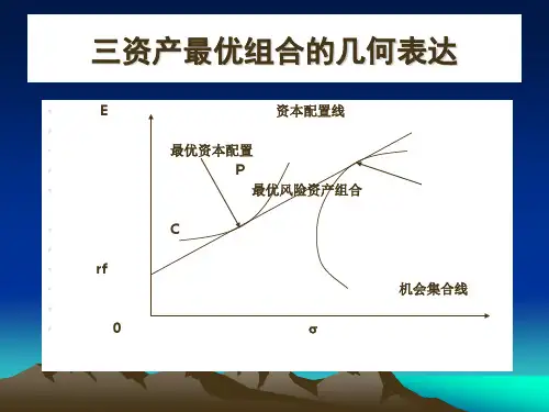
2、资本配置线正是由于无风险资产引入,才可以形成无风险资产和风险资产之间的资本配置线CAL(capital allocation line,CAL),但是CAL仅仅为风险资产和无风险组合的“一般搭配”,并非“最优搭配”;而市场组合M与无风险资产构成全部资产组合的集合形成资本市场线(CML),是与“有效边界”相切的资本配置线,是一种“最优的”资本配置线。
3、市盈率增长因子(PEG)市盈率增长因子(PEG)是对P/E静态性缺陷的重要补充。
PEG是将一只股票的市盈率除以该公司的成长性。
其中,用估计盈利增长率除市盈率可以测算公司成长的速度,这就是著名的预期市盈率增长因子(Prospective PEG)。
市盈率增长因子越低,表示公司的发展潜力越大,公司的潜在价值也就越高。
市盈率/公司利润增长率,大于1说明估值高;小于1说明便宜。
4、动量效应投资者行为的研究表明,股票上涨得越多,就有也越多的投资者认为它继续上涨,因而股价的上涨存在一种自我实现机制,即存在动量效应(momentum effect)。
在股价的正反馈机制中,噪声交易这对股价上涨起到推动作用,而明智的专业投资者将从噪声交易者的追逐动能效应策略的过程中获取收益。
投资学讲义免费的商务管理资料平台第一章財務管理概論恐龍蛋遊戲軟體設計公司,前一陣子推出「水滸傳」網路遊戲軟體。
這個公司成立迄今已有三年,已推出四個頗受市場歡迎的遊戲軟體,公司預計本年度的營收將達2億元。
目前,這家公司資本額為2千萬元,此外,為了籌措營運所需資金,公司準備將自有的廠房及倉庫抵押給銀行以取得4千萬元擔保放款。
這家公司還計畫進一步將營業項目擴展到商用以及教育應用軟體的開發設計。
為因應這些擴充計劃,公司財務副總經理發現現有的資金籌措方式將不足以應付未來公司對資金的需求。
更嚴重的是,公司將立即面臨短期營運現金不足的問題。
這家公司所面臨的幾個問題也正是財務管理這門課所關注的課題:(1)這家公司的未來投資策略應是什麼?(即,這家公司為何要進入商用及教育應用軟體的開發與生產?)如何評估並選擇最佳的投資計劃?(即,錢怎麼投資?)(2)一旦選定投資計畫,公司如何籌措投資計畫所需的資金?(即,錢從那裡來?)(3)這家公司日常營運需要多少週轉金?(即,如何管理現金?)企業選擇最適的投資策略前,必須先確立企業的經營目標。
選定後,經營目標的達成須借助投資計畫的評估,選擇以及執行。
投資計畫的評估,選擇就是投資決策的範疇。
投資決策(或稱資本預算決策,capital budgeting decisions),就是將公司資本支出預算用於購置公司營運所需的固定資產(如:廠房、機器設備)以及無形資產(如:商譽、商標及專利權),而公司經營目標就是追求所購置的資產創造最大的價值且必須大於資本支出。
亦即,若企業投資決策的目標是追求所購置的資產所創造的淨價值最大,則企業經營績效勢必取決於各項投資計畫能為股東創造多少的價值?故企業營運最終的目標就應是追求企業所有人所增加的財富極大。
1. 何謂財務管理?假設朱一決定自行創業成立公司生產CPU專用的散熱風扇。
公司設立前,朱一必須聘請會計、財務以及採購管理人員負責採購生產原物料以及財務、人事管理,找到合適的廠房、機器設備,並招募到足夠的工人從事生產。
Chapter 13 Factor pricing modelFan LongzhenIntroduction•The consumption-based model as a complete answer to most asset pricing question in principle, does not work well in practice;•This observation motivates effects to tie the discount factor m to other data;•Linear factor pricing models are most popular models of this sort in finance;•They dominate discrete-time empirical work.Factor pricing models•Factor pricing models replace the consumption-based expression for marginal utility growth with a linear model of the form•The key question: what should one use for factors 11'+++=t t f b a m 1+t fCapital asset pricing model (CAPM)•CAPM is the model , is the wealth portfolio return.•Credited Sharpe (1964) and Linterner (1965), is the first, most famous, and so far widely used model in asset pricing.•Theoretically, a and b are determined to price any two assets, such as market portfolio and risk free asset.•Empirically, we pick a,b to best price larger cross section of assets;•We don’t have good data, even a good empirical definition for wealth portfolio, it is often deputed by a stock index;•We derive it from discount factor model by •(1)two-periods, exponential utility, and normal returns; •(2) infinite horizon, quadratic utility, and normal returns;•(3) log utility •(4) by seeing several derivations, you can see how one assumption can be traded for another. For example, the CAPM does not require normal distributions, if one is willing to swallow quadratic utility instead.wbR a m +=w RExponential utility, Normal distributions•We present a model with consumption only in the last period, utility is•If consumption is normally distributed, we have •Investor has initial wealth w, which invest in a set of risk-free assets with return and a set of risky assets paying return R.•Let y denote the mount of wealth w invested in each asset, the budget constraint is •Plugging the first constraint into the utility function, we obtain][)]([c eE c U E α−−=2/)()(22))((c c E e c U E σαα+−−=f R f y y w Ry R y c ff f ''+=+=yy R E y R y f f e c U E Σ++−−='2/)]('[2))((ααExponential utility, Normal distributions--continued •Applying the formula to market return itself, we have•The model ties price of market risk to the risk aversion coefficient.)()(2wf w R R R E ασ=−Quadratic value function, Dynamicprogramming-continued•(1) the value function only depends on wealth. If other variables enter the value function, m would depend on other variables. The ICAPM, allows other variables in the value function, and obtain more factors.•(other variable can enter the function, so long as they do not affect marginal utility value of wealth.)•(2) the value function is quadratic, we wanted the marginal value function is linear.Why is the value function quadratic•Good economists are unhappy about a utility function that have wealth in it.•Suppose investors last forever, and have the standard sort of utility function •Investors start with wealth which earns a random return andhave no other source of income;•Suppose further that interest rate are constant and stock returns are iid over time.•Define the value function as the maximized value of the utility function in this environment•∑∞=+=0)(j j t jt c u E U β0w w R {}11;);(..)()(''110,...,...,,max11==−==++∞=+∑++vtt tw tt t w t t j j t jt w w c c t R R c W R W t s c u E W V t t t t ωωβ,Why is the value function quadratic--continued•Without the assumption of no labor income, a constant interest rate, and I.I.d returns come in, the value maybe depend on the environment.For example, if D/P indicates returns would be high for a while, the investor might be happier and have a high value.•Value functions allow you to express an infinite-period problem as a two-period problem. Breaking up the maximization into the first period and the remaining periods, as follows•Or{}{}⎪⎭⎪⎬⎫⎪⎩⎪⎨⎧⎥⎦⎤⎢⎣⎡+=∑∞=+++++++11,...,,...,,,)()()(maxmax2121jjtjtwwccttwctcuEEcuWVttttttββ{}{})()()(1,max++=tttwctWVEcuWVttβLinearizing any model •Goal of linear model: derive variables that drive the discount factor; derive a linear relation between discount factor and these variables;•Following gives three standard tricks to obtain a linear model;Linearizing any model-Talyorexpansion•From •We have)(11++=ttfgm))())((('))((11111+++++−+≈ttttttttfEffEgfEgmComments on the CAPM and ICAPM•Is CAPM conditional or unconditional? Are the parameter changes as conditional information changes ?•The two-period quadratic utility-based deviation results in a conditional CAPM, since the parameters change over time.•The log utility CAPM hold both conditionally or unconditionally.•Should CAPM price options? The quadratic utility CAPM and log utility CAPM should apply to all payoffs.•Why linearize? Why not take the log utility model whichshould price any asset? Turn it into cannot price no normally distributed payoff and must be applied at short horizons.•it is simple to use regression to estimate in CAPM.•Now with GMM approach, nolinear discount factor model is easy to estimate.tt b a ,W R m /1=W t t t t R b a m 11+++=γβ,Comments on the CAPM and ICAPM---continued •Identify the factors: it is a art!。


复旦大学2024年春季基础班测试卷投资学(A)一、单项选择题(每题2分,共30分)1、我国成立的第一个公司制的证券交易所是()。
A.上海证券交易所B.深圳证券交易所C.香港证券交易所D.北京证券交易所2、下列说法正确的是()。
A.用贴现现金流模型计算证券内在价值时,当计算的内部收益率大于必要收益率时,不可以考虑购买这种证券B.用贴现现金流模型计算证券内在价值时,当计算的内部收益率小于必要收益率时,可以考虑购买这种证券C.零增长模型假定对某种股票永远支付固定的股利D.不变增长模型是零增长模型的一个特例3、一张期限为5年的付息债券,票面利率为7%,现在的到期收益率是8%,如果利率保持不变,则一年后的债券价格将()。
A.不变B.更高C.更低D.无法判断4、A、B、C三只股票具有相同的期望收益率和方差,下表为三只股票收益之间的相关C.平均投资于B和CD.全部投资于C5、一位投资者希望构造一个资产组合,并且资产组合的位置在资本配置线上最优风险资产组合的右边,那么()。
A.以无风险资产贷出部分资金,剩余资金投入最优无风险资产B.以无风险利率借入部分资金,剩余部分投入最优风险资产组合C.只投入最优风险资产D.不可能有这样的资产组合6、下列哪一个不属于弱式有效市场假说的检验?()A.相关性检验B.游程检验C.过滤法则检验D.事件研究检验7、近年来,美国经济逐渐从经济危机中复苏过来,根据美林投资钟模型,复苏阶段的最佳资产类别是()。
A.国债B.股票C.大宗商品D.现金8、一个债券的当前价格是98.6,到期收益率为3%,假设到期收益率上升0.3个百分点,债券价格下降到97.4,则此债券的修正久期是()。
A.4.0568B.3.9386C.4.1785D.4.25679、P研究机构正在进行一项覆盖成熟制造行业的调查。
特许金融分析师托尼是这家研根据这些基础数据计算行业的市盈率(P0/E1)为()。
A.10B.15C.20D.3010、夏普指数高表明()。
Chapter 15 the equity market (cross-section patternsand time-series patterns)Fan LongzhenIntroduction•In this class, we again look at the stock return data, but with a very different view point;•Previously, we examined the data through the “eyes”of CAPM. We had a noble intension, although it didn’t work very well;•Now we are going to get our hands “dirty”, and plunge right into the data, without a formal model;•In particular, we will look at some well-established patterns---size,value, and momentum—that have beensuccessful in explaining the cross-sectional stock returns.Multifactor-regressions•For each asset i, we use a multi-factor time-series regression to quantify the asset’s tendency to move with multiple risk factors:• 1. Systematic factors:•:risk premium•:risk premium • 2 idiosyncratic factors:•: no risk premium • 3. Factor loadings:•beta(i): sensitivity to market risk;•: sensitivity to the factor risk.i tt i f t M t i i f t i t e F f r r r r ++−+=−)(βαM t r )(f t M t M r r E −=λtF )(t F F E =λi t e 0)(=i t e E i fThe pricing relation•Given the risk premia of the systematic factors, the determinants of expected returns:•What are the additional systematic factors?FiM i f t i t f r r E λλβ+=−)(Size: small or big•We sort the socks by their market capitalization: share price* number of shares outstandingValue or growth•We can sort the cross-section of stocks by their book-to-market ratios: growth stocks:firm with low book-to-market ratios;•Value stocks:firms with high book-to-market ratios.Other factors•Price-to-earining ratios,•The market skewness fcator•---Havey and Siddique(JF,2000) report that systematic skewness is economically important and commands an average risk premium of 3.6% per year.Time-series behavior•For the time-series behavior of stock returns, we focus in particular on the time-varying nature of expected return and volatility;•We are interested in building dynamic models that explicitly incorporate conditioning information to best describe the behavior of future stock returns.Predictability and marketefficiency•In addition to the random walk test, there is mounting evidence that stock returns are predictable;•Some argue that predictability implies market inefficiency. What do you think?•Others contend it is simple a result of rational variation in expected returns;•Suppose this is true. Can we find a coherent story that relates the variation through time of expected returns to business conditionsWhat cause expected returns to vary?•Using the intuition of CAPM, expected returns canvary for two reasons:• 1. Varying risk aversion;• 2. Varying exposure to market risk, or varying market risk.•When income is high, investor want save more, higher saving lead to lower expected returns;•Empirical implication?Variables related to business condition •Default spreads: difference in yields between defaultable bonds and treasury bonds with similar maturities. When the business condition is bad, the systematic default risk increases, widening the default spread.•Term premiums: difference in yields between long-and short-term treasury bonds. This is a forward-looking variable predictive of future inflation, and is found to be important in forecasting real economic activity.•Financial ratios: book-to-market, dividend yields, ect. Variables that are important in fundamental valuationTime-varying volatility---volatility also changes with time •If the rate of information arrival is time-varying, so is the rate of price adjustment, causing the volatility to change over time;•The time-varying volatility of the market return is related to the time-varying volatility of a variety of economic variables, includinginflation, money growth, and industrial production;•Stock market volatility increases with financial leverage: a decrease in stock price causes an increase in financial leverage, cause volatility to increase;•Investors’s sudden changes of risk attitudes, changes in market liquidity, and temporary imbalance of supply and demand could all cause market volatility to change over time.•What are the testable empirical implications?Stochastic volatility•More generally, volatility is a stochastic process of its own, this is an active area of research in academics and in industry.•Some well-known facts about stochastic volatility:• 1. It is persistent: volatile periods are followed by volatile periods;• 2. It is mean-reverting: over time, volatility converges to its long-run mean.• 3. There is a negative correlation between volatility and return: large negative price jumps are coupled with large positive volatility jumps.。
2015年复旦大学金融硕士(MF)金融学综合真题试卷(题后含答案及解析)题型有:1. 单项选择题 2. 名词解释 3. 计算题 4. 简答题 5. 论述题单项选择题1.根据CAPM模型,假定市场组合收益率为15%,无风险利率为6%,某证券的贝塔系数为1.2,期望收益率为18%,则该证券( )。
A.被高估B.被低估C.合理估值D.以上都不对正确答案:B解析:根据CAPM模型,该证券的必要报酬率=6%+1.2×(15%-6%)=16.8%<18%,即该证券的期望收益率高于必要报酬率,实际价格被低估。
故选B。
2.货币市场的主要功能是( )。
A.短期资金融通B.长期资金融通C.套期保值D.投机正确答案:A解析:货币市场是指以期限在1年以内的金融工具为媒介进行短期资金融通的市场。
其主要功能是短期资金融通。
故选A。
3.国际收支平衡表中将投资收益计入( )。
A.贸易收支B.经常账户C.资本账户D.官方储备正确答案:B解析:在国际收支平衡表中,经常账户包括货物、服务、收入和经常转移。
其中,收入包括职工的报酬和投资收益两类交易。
故选B。
4.下列说法不正确的是( )。
A.当央行进行正回购交易时,商业银行的超额准备金将减少;当央行进行逆回购交易时,商业银行的超额准备金将增加B.法定准备金率对货币供给的影响与公开市场操作及贴现率不同,后两者主要针对基础货币进行调控,法定准备金则直接作用于货币乘数C.法定准备金作为货币政策工具的历史长于其作为稳定金融、防止流动性危机的政策工具D.公开市场操作的有效性受国内金融市场的发达程度影响正确答案:C解析:实行准备金的目的是为了确保商业银行在遇到突然大量提取银行存款时,能有相当充足的清偿能力。
自20世纪30年代以后,法定准备金制度才成为国家调节经济的重要手段,是中央银行对商业银行的信贷规模进行控制的一种制度。
故选C。
5.甲公司现有流动资产500万元(其中速动资产200万元),流动负债200万元。
Chapter 14 The CAPM ---Applications and
tests
Fan Longzhen
Predictions and applications •CAPM: in market equilibrium, investors are only rewarded for bearing
the market risk;
•APT: in the absence of arbitrage, investors are only rewarded for bearing the factor risk;
•Applications:
•---professional portfolio managers: evaluating security returns and fund performance
•---corporate manager: capital budgeting decisions.
Testability of CAPM
•The wide acceptance of the CAPM and APT makes it all more important to test their predictions empirically.•How does a product of abstract reasoning hold in reality?•Unfortunately, the predictions of the CAPM and APT are hard to test empirically
•---neither the market portfolio in CAPM nor the risk factor in APT is observable;
•---expected returns are unobservable, and could be time-varying;
•---volatility is not directly observable, and is time-varying.
An ideal test of the CAPM
•In an idea situation, we have the following input:
• 1. Risk-free borrowing/lending rate ;
• 2. Expected returns on the market and on the risky asset ;• 3. The exposure to market risk ; •These input allow us to examine the relation between reward •and risk :• 1. More risk, more reward?• 2. Do they line up?
• 3. What is the reward for a risk exposure of 1?•
4. Zero risk, zero reward?
f R )(M R E )(i R E )
var(/),cov(M i M i R R R =β))((f i R R E −i
β
Testing the linear relation
•Pick a proxy for the market portfolio, and record N monthly returns:
•For the same sample period, collect a sample of I firms, each with N monthly returns:•Construct sample estimates •For , test the linear relation:
•N
t R M t ,...,2,1:=N t and I i R i t ,...,2,1,...,2,1:==i
M i m m βˆ,ˆ,ˆI i ,...,2,1=i
f i R m βγγˆˆ10+=−
Implication of the CAPM and testing
•Implication of CAPM: with •
: zero exposure, zero reward;•: one unit of exposure, the same reward as the market.•With 43 industrial portfolios, the test tells us that this relation does not hold exactly.
•One possibility: our measures of the expected returns are contaminated by noises that are unrelated to the beta’s;
•What we still would like to know:•---on average, is reward related to risk at all? Or not?•---On average, does zero risk results in zero reward? ? Or not?•---on average, does one unit of risk exposure pay market return?•or not i f i R m βγγˆˆ10+=−00=γf M R m
−=ˆ1γ01=γ00=γ%9.5ˆ1=−=f M R m
γ
A summary of the CAPM tests •In general, the test results depend on the sample data, sample periods, statistical approaches, proxy for the market portfolio, ect. But the
following findings remain robust:
•the relation between risk and reward is much flatter than that predicted by the CAPM;
•The risk beta can not even to begin to explain the cross-sectional variation in the expected returns;
•Contrary to the prediction of the CAPM, the intercept is significant different from zero.
Some possible explanations
• 1. Is the stock market index a good proxy for the market portfolio?
•Only 1/3 non-governmental tangible assets are owned by the corporate sector;•Among the corporate assets, only 1/3 are financed by equity
•What are about intangible assets, like human capital;
•What about international markets?
• 2. Measurement error in beta
•Except for the market portfolio, we never observe the true beta;
•To test CAPM, we use estimates for beta, which are measured with errors • 3. Measurement error in expected returns
•We use sample mean as the unobservable expected returns;
•There are noises in our estimates;
•Is the noises are correlated, then we have a statistical problem(error-in-variables)
• 4. Borrowing restrictions
•Fisher black showed that borrowing restrictions might cause low-beta stocks to have higher expected returns than the CAPM predicts.
Going beyond the CAPM •Is beta a good measure of risk exposure? What about the risk
associated with negative skewness?
•Could there be other risk factors?
•Time-varying volatility,
•Time-varying expected returns,
•Time –varying risk aversion,
•And time-varying beta?。