数学建模多目标规划函数fgoalattain

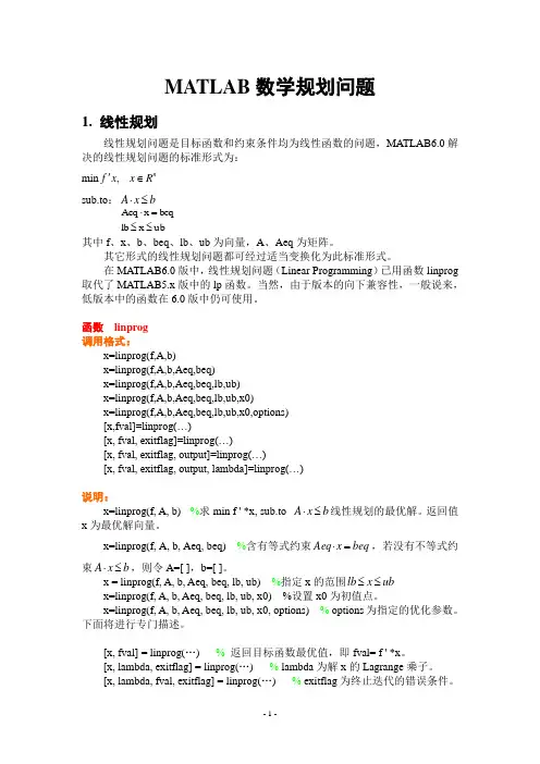
MATLAB数学规划问题1. 线性规划线性规划问题是目标函数和约束条件均为线性函数的问题，MATLAB6.0解决的线性规划问题的标准形式为：',min n Rf∈xxsub.to：b⋅xA≤A e q=⋅xb e q≤lb≤xub其中f、x、b、beq、lb、ub为向量，A、Aeq为矩阵。

其它形式的线性规划问题都可经过适当变换化为此标准形式。

在MATLAB6.0版中，线性规划问题（Linear Programming）已用函数linprog 取代了MATLAB5.x版中的lp函数。

当然，由于版本的向下兼容性，一般说来，低版本中的函数在6.0版中仍可使用。

函数linprog调用格式：x=linprog(f,A,b)x=linprog(f,A,b,Aeq,beq)x=linprog(f,A,b,Aeq,beq,lb,ub)x=linprog(f,A,b,Aeq,beq,lb,ub,x0)x=linprog(f,A,b,Aeq,beq,lb,ub,x0,options)[x,fval]=linprog(…)[x, fval, exitflag]=linprog(…)[x, fval, exitflag, output]=linprog(…)[x, fval, exitflag, output, lambda]=linprog(…)说明：x=linprog(f, A, b)%求min f ' *x, sub.to bA≤⋅线性规划的最优解。

返回值xx为最优解向量。

x=linprog(f, A, b, Aeq, beq) %含有等式约束beq⋅，若没有不等式约Aeq=x束b⋅，则令A=[ ]，b=[ ]。

A≤xx = linprog(f, A, b, Aeq, beq, lb, ub) %指定x的范围ub≤lb≤xx=linprog(f, A, b, Aeq, beq, lb, ub, x0) %设置x0为初值点。

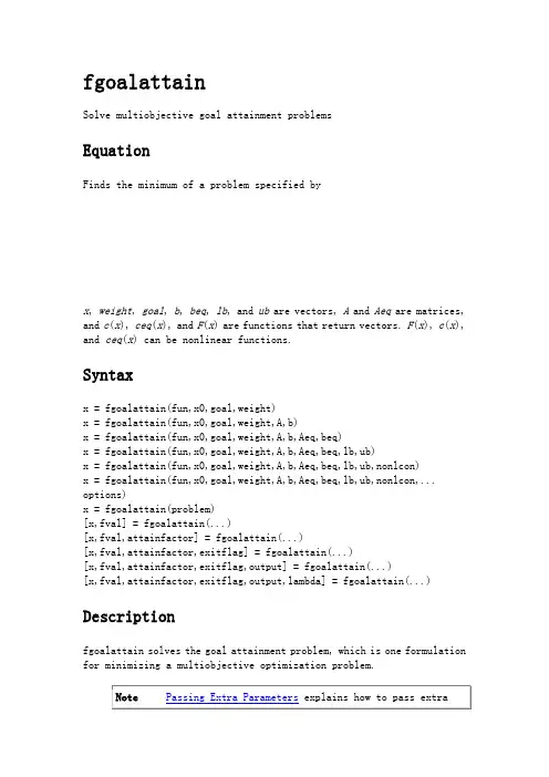
fgoalattainSolve multiobjective goal attainment problemsEquationFinds the minimum of a problem specified byx, weight, goal, b, beq, lb, and ub are vectors, A and Aeq are matrices, and c(x), ceq(x), and F(x) are functions that return vectors. F(x), c(x), and ceq(x) can be nonlinear functions.Syntaxx = fgoalattain(fun,x0,goal,weight)x = fgoalattain(fun,x0,goal,weight,A,b)x = fgoalattain(fun,x0,goal,weight,A,b,Aeq,beq)x = fgoalattain(fun,x0,goal,weight,A,b,Aeq,beq,lb,ub)x = fgoalattain(fun,x0,goal,weight,A,b,Aeq,beq,lb,ub,nonlcon)x = fgoalattain(fun,x0,goal,weight,A,b,Aeq,beq,lb,ub,nonlcon,... options)x = fgoalattain(problem)[x,fval] = fgoalattain(...)[x,fval,attainfactor] = fgoalattain(...)[x,fval,attainfactor,exitflag] = fgoalattain(...)[x,fval,attainfactor,exitflag,output] = fgoalattain(...)[x,fval,attainfactor,exitflag,output,lambda] = fgoalattain(...)Descriptionfgoalattain solves the goal attainment problem, which is one formulation for minimizing a multiobjective optimization problem.x = fgoalattain(fun,x0,goal,weight) tries to make the objective functions supplied by fun attain the goals specified by goal by varying x, starting at x0, with weight specified by weight.x = fgoalattain(fun,x0,goal,weight,A,b) solves the goal attainment problem subject to the linear inequalities A*x ≤ b.x = fgoalattain(fun,x0,goal,weight,A,b,Aeq,beq) solves the goal attainment problem subject to the linear equalities Aeq*x = beq as well. Set A = [] and b = [] if no inequalities exist.x = fgoalattain(fun,x0,goal,weight,A,b,Aeq,beq,lb,ub) defines a set of lower and upper bounds on the design variables in x, so that the solution is always in the range lb ≤ x ≤ ub.x = fgoalattain(fun,x0,goal,weight,A,b,Aeq,beq,lb,ub,nonlcon) subjects the goal attainment problem to the nonlinear inequalities c(x) or nonlinear equality constraints ceq(x) defined in nonlcon. fgoalattain optimizes such that c(x) ≤ 0 and ceq(x) = 0. Set lb = [] and/or ub = [] if no bounds exist.x = fgoalattain(fun,x0,goal,weight,A,b,Aeq,beq,lb,ub,nonlcon,... options) minimizes with the optimization options specified in the structure options. Use optimset to set these options.x = fgoalattain(problem) finds the minimum for problem, where problem is a structure described in Input Arguments.Create the structure problem by exporting a problem from Optimization Tool, as described in Exporting to the MATLAB Workspace.[x,fval] = fgoalattain(...) returns the values of the objective functions computed in fun at the solution x.[x,fval,attainfactor] = fgoalattain(...) returns the attainment factor at the solution x.[x,fval,attainfactor,exitflag] = fgoalattain(...) returns a value exitflag that describes the exit condition of fgoalattain.[x,fval,attainfactor,exitflag,output] = fgoalattain(...) returns a structure output that contains information about the optimization.[x,fval,attainfactor,exitflag,output,lambda] = fgoalattain(...) returns a structure lambda whose fields contain the Lagrange multipliers at the solution x.Input ArgumentsFunction Arguments contains general descriptions of arguments passed into fgoalattain. This section provides function-specific details for fun, goal, nonlcon, options, weight, and problem:fun The function to be minimized. fun is a function that acceptsa vector x and returns a vector F, the objective functionsevaluated at x. The function fun can be specified as a functionhandle for a function file:x = fgoalattain(@myfun,x0,goal,weight)where myfun is a MATLAB function such asfunction F = myfun(x)F = ... % Compute function values at x.fun can also be a function handle for an anonymous function.x = fgoalattain(@(x)sin(x.*x),x0,goal,weight);If the user-defined values for x and F are matrices, they areconverted to a vector using linear indexing.To make an objective function as near as possible to a goalvalue, (i.e., neither greater than nor less than) use optimsetto set the GoalsExactAchieve option to the number of objectivesrequired to be in the neighborhood of the goal values. Suchobjectives must be partitioned into the first elements of thevector F returned by fun.If the gradient of the objective function can also be computedand the GradObj option is 'on', as set byoptions = optimset('GradObj','on')then the function fun must return, in the second outputargument, the gradient value G, a matrix, at x. The gradientconsists of the partial derivative dF/dx of each F at the pointx. If F is a vector of length m and x has length n, where n isthe length of x0, then the gradient G of F(x) is an n-by-m matrixwhere G(i,j) is the partial derivative of F(j) with respect tox(i) (i.e., the jth column of G is the gradient of the jthobjective function F(j)).goal Vector of values that the objectives attempt to attain. The vector is the same length as the number of objectives F returnedby fun. fgoalattain attempts to minimize the values in thevector F to attain the goal values given by goal.nonlcon The function that computes the nonlinear inequality constraints c(x) ≤ 0 and the nonlinear equality constraintsceq(x) = 0. The function nonlcon accepts a vector x and returnstwo vectors c and ceq. The vector c contains the nonlinearinequalities evaluated at x, and ceq contains the nonlinearequalities evaluated at x. The function nonlcon can bespecified as a function handle.x = fgoalattain(@myfun,x0,goal,weight,A,b,Aeq,beq,...lb,ub,@mycon)where mycon is a MATLAB function such asfunction [c,ceq] = mycon(x)c = ... % compute nonlinear inequalities at x.ceq = ... % compute nonlinear equalities at x.If the gradients of the constraints can also be computed andthe GradConstr option is 'on', as set byoptions = optimset('GradConstr','on')then the function nonlcon must also return, in the third andfourth output arguments, GC, the gradient of c(x), and GCeq,the gradient of ceq(x). Nonlinear Constraints explains how to"conditionalize" the gradients for use in solvers that do notaccept supplied gradients.If nonlcon returns a vector c of m components and x has lengthn, where n is the length of x0, then the gradient GC of c(x)is an n-by-m matrix, where GC(i,j) is the partial derivativeof c(j) with respect to x(i) (i.e., the jth column of GC is thegradient of the jth inequality constraint c(j)). Likewise, ifceq has p components, the gradient GCeq of ceq(x) is an n-by-pmatrix, where GCeq(i,j) is the partial derivative of ceq(j)with respect to x(i) (i.e., the jth column of GCeq is thegradient of the jth equality constraint ceq(j)).Passing Extra Parameters explains how to parameterize thenonlinear constraint function nonlcon, if necessary.options Options provides the function-specific details for the options values.weight A weighting vector to control the relative underattainment or overattainment of the objectives in fgoalattain. When thevalues of goal are all nonzero, to ensure the same percentageof under- or overattainment of the active objectives, set theweighting function to abs(goal). (The active objectives are theset of objectives that are barriers to further improvement ofthe goals at the solution.)When the weighting function weight is positive, fgoalattainattempts to make the objectives less than the goal values. Tomake the objective functions greater than the goal values, setweight to be negative rather than positive. To make an objectivefunction as near as possible to a goal value, use theGoalsExactAchieve option and put that objective as the firstelement of the vector returned by fun (see the precedingdescription of fun and options).problem objective Vector of objective functionsx0 Initial point for xgoal Goals to attainweight Relative importance factors of goalsAineq Matrix for linear inequality constraintsbineq Vector for linear inequality constraintsAeq Matrix for linear equality constraintsbeq Vector for linear equality constraintslb Vector of lower boundsub Vector of upper boundsnonlcon Nonlinear constraint functionsolver 'fgoalattain'options Options structure created with optimset Output ArgumentsFunction Arguments contains general descriptions of arguments returned by fgoalattain. This section provides function-specific details for attainfactor, exitflag, lambda, and output:attainfactor The amount of over- or underachievement of the goals. If attainfactor is negative, the goals have been overachieved;if attainfactor is positive, the goals have beenunderachieved.attainfactor contains the value of γ at the solution. Anegative value of γindicates overattainment in the goals.exitflag Integer identifying the reason the algorithm terminated.The following lists the values of exitflag and thecorresponding reasons the algorithm terminated.1 Function converged to a solutions x.4 Magnitude of the search direction lessthan the specified tolerance andconstraint violation less thanoptions.TolCon5 Magnitude of directional derivative lessthan the specified tolerance andconstraint violation less thanoptions.TolCon0 Number of iterations exceededoptions.MaxIter or number of functionevaluations exceeded options.FunEvals-1 Algorithm was terminated by the outputfunction.-2 No feasible point was found.lambda Structure containing the Lagrange multipliers at the solution x (separated by constraint type). The fields of thestructure arelower Lower bounds lbupper Upper bounds ubineqlin Linear inequalitieseqlin Linear equalitiesineqnonlin Nonlinear inequalitieseqnonlin Nonlinear equalitiesoutput Structure containing information about the optimization.The fields of the structure areiterations Number of iterations takenfuncCount Number of function evaluationslssteplength Size of line search step relative tosearch directionstepsize Final displacement in xalgorithm Optimization algorithm usedfirstorderopt Measure of first-order optimalityconstrviolation Maximum of constraint functionsmessage Exit messageOptionsOptimization options used by fgoalattain. You can use optimset to set or change the values of these fields in the options structure options. See Optimization Options for detailed information.DerivativeCheck Compare user-supplied derivatives (gradients ofobjective or constraints) to finite-differencingderivatives. The choices are 'on' or the default,'off'.Diagnostics Display diagnostic information about the functionto be minimized or solved. The choices are 'on' orthe default, 'off'.DiffMaxChange Maximum change in variables for finite-differencegradients (a positive scalar). The default is 0.1.DiffMinChange Minimum change in variables for finite-differencegradients (a positive scalar). The default is 1e-8. Display Level of display.∙'off' displays no output.∙'iter' displays output at each iteration, andgives the default exit message.∙'iter-detailed' displays output at eachiteration, and gives the technical exitmessage.∙'notify' displays output only if the functiondoes not converge, and gives the default exitmessage.∙'notify-detailed' displays output only if thefunction does not converge, and gives thetechnical exit message.∙'final' (default) displays just the finaloutput, and gives the default exit message.∙'final-detailed' displays just the finaloutput, and gives the technical exit message.FinDiffType Finite differences, used to estimate gradients, areeither 'forward' (default), or 'central'(centered). 'central' takes twice as many functionevaluations, but should be more accurate.The algorithm is careful to obey bounds whenestimating both types of finite differences. So, forexample, it could take a backward, rather than aforward, difference to avoid evaluating at a pointoutside bounds.FunValCheck Check whether objective function and constraintsvalues are valid. 'on' displays an error when theobjective function or constraints return a valuethat is complex, Inf, or NaN. The default, 'off',displays no error.GoalsExactAchieve Specifies the number of objectives for which it isrequired for the objective fun to equal the goal goal(a nonnegative integer). Such objectives should bepartitioned into the first few elements of F. Thedefault is 0.GradConstr Gradient for nonlinear constraint functions definedby the user. When set to 'on', fgoalattain expectsthe constraint function to have four outputs, asdescribed in nonlcon in the Input Arguments section.When set to the default, 'off', gradients of thenonlinear constraints are estimated by finitedifferences.GradObj Gradient for the objective function defined by theuser. See the preceding description of fun to seehow to define the gradient in fun. Set to 'on' tohave fgoalattain use a user-defined gradient of theobjective function. The default, 'off',causesfgoalattain to estimate gradients usingfinite differences.MaxFunEvals Maximum number of function evaluations allowed (apositive integer). The default is100*numberOfVariables.MaxIter Maximum number of iterations allowed (a positiveinteger). The default is 400.MaxSQPIter Maximum number of SQP iterations allowed (a positiveinteger). The default is 10*max(numberOfVariables,numberOfInequalities + numberOfBounds)MeritFunction Use goal attainment/minimax merit function if setto 'multiobj', the default. Use fmincon meritfunction if set to 'singleobj'.OutputFcn Specify one or more user-defined functions that anoptimization function calls at each iteration,either as a function handle or as a cell array offunction handles. The default is none ([]). SeeOutput Function.PlotFcns Plots various measures of progress while thealgorithm executes, select from predefined plots orwrite your own. Pass a function handle or a cellarray of function handles. The default is none ([]).∙@optimplotx plots the current point∙@optimplotfunccount plots the function count∙@optimplotfval plots the function value∙@optimplotconstrviolation plots the maximumconstraint violation∙@optimplotstepsize plots the step sizeFor information on writing a custom plot function,see Plot Functions.RelLineSrchBnd Relative bound (a real nonnegative scalar value) onthe line search step length such that the totaldisplacement in x satisfies|Δx(i)| ≤relLineSrchBnd· max(|x(i)|,|typicalx(i)|). This option provides control over themagnitude of the displacements in x for cases inwhich the solver takes steps that are considered toolarge. The default is none ([]).RelLineSrchBndDurat ion Number of iterations for which the bound specified in RelLineSrchBnd should be active (default is 1).TolCon Termination tolerance on the constraint violation,a positive scalar. The default is 1e-6.TolConSQP Termination tolerance on inner iteration SQPconstraint violation, a positive scalar. Thedefault is 1e-6.TolFun Termination tolerance on the function value, apositive scalar. The default is 1e-6.TolX Termination tolerance on x, a positive scalar. Thedefault is 1e-6.TypicalX Typical x values. The number of elements in TypicalXis equal to the number of elements in x0, thestarting point. The default value isones(numberofvariables,1). fgoalattain usesTypicalX for scaling finite differences forgradient estimation.UseParallel When 'always', estimate gradients in parallel.Disable by setting to the default, 'never'. ExamplesConsider a linear system of differential equations.An output feedback controller, K, is designed producing a closed loop systemThe eigenvalues of the closed loop system are determined from the matrices A, B, C, and K using the command eig(A+B*K*C). Closed loop eigenvalues must lie on the real axis in the complex plane to the left of the points [-5,-3,-1]. In order not to saturate the inputs, no element in K can be greater than 4 or be less than -4.The system is a two-input, two-output, open loop, unstable system, with state-space matrices.The set of goal values for the closed loop eigenvalues is initialized as goal = [-5,-3,-1];To ensure the same percentage of under- or overattainment in the active objectives at the solution, the weighting matrix, weight, is set to abs(goal).Starting with a controller, K = [-1,-1; -1,-1], first write a function file, eigfun.m.function F = eigfun(K,A,B,C)F = sort(eig(A+B*K*C)); % Evaluate objectivesNext, enter system matrices and invoke an optimization routine.A = [-0.5 0 0; 0 -2 10; 0 1 -2];B = [1 0; -2 2; 0 1];C = [1 0 0; 0 0 1];K0 = [-1 -1; -1 -1]; % Initialize controller matrixgoal = [-5 -3 -1]; % Set goal values for the eigenvalues weight = abs(goal); % Set weight for same percentagelb = -4*ones(size(K0)); % Set lower bounds on the controllerub = 4*ones(size(K0)); % Set upper bounds on the controller options = optimset('Display','iter'); % Set display parameter[K,fval,attainfactor] = fgoalattain(@(K)eigfun(K,A,B,C),...K0,goal,weight,[],[],[],[],lb,ub,[],options)You can run this example by using the demonstration script goaldemo. (From the MATLAB Help browser or the MathWorks™ Web site documentation, you can click the demo name to display the demo.) After about 11 iterations, a solution isActive inequalities (to within options.TolCon = 1e-006):lower upper ineqlinineqnonlin1 12 24K =-4.0000 -0.2564-4.0000 -4.0000fval =-6.9313-4.1588-1.4099attainfactor =-0.3863DiscussionThe attainment factor indicates that each of the objectives has been overachieved by at least 38.63% over the original design goals. The active constraints, in this case constraints 1 and 2, are the objectives that are barriers to further improvement and for which the percentage of overattainment is met exactly. Three of the lower bound constraints are also active.In the preceding design, the optimizer tries to make the objectives less than the goals. For a worst-case problem where the objectives must be as near to the goals as possible, use optimset to set the GoalsExactAchieve option to the number of objectives for which this is required.Consider the preceding problem when you want all the eigenvalues to be equal to the goal values. A solution to this problem is found by invoking fgoalattain with the GoalsExactAchieve option set to 3.options = optimset('GoalsExactAchieve',3);[K,fval,attainfactor] = fgoalattain(...@(K)eigfun(K,A,B,C),K0,goal,weight,[],[],[],[],lb,ub,[],... options)After about seven iterations, a solution isK =-1.5954 1.2040-0.4201 -2.9046fval =-5.0000-3.0000-1.0000attainfactor =1.0859e-20In this case the optimizer has tried to match the objectives to the goals. The attainment factor (of 1.0859e-20) indicates that the goals have been matched almost exactly.NotesThis problem has discontinuities when the eigenvalues become complex; this explains why the convergence is slow. Although the underlying methods assume the functions are continuous, the method is able to make stepstoward the solution because the discontinuities do not occur at the solution point. When the objectives and goals are complex, fgoalattain tries to achieve the goals in a least-squares sense.AlgorithmMultiobjective optimization concerns the minimization of a set of objectives simultaneously. One formulation for this problem, and implemented in fgoalattain, is the goal attainment problem of Gembicki[3]. This entails the construction of a set of goal values for the objective functions. Multiobjective optimization is discussed in Multiobjective Optimization.In this implementation, the slack variable γis used as a dummy argument to minimize the vector of objectives F(x) simultaneously; goal is a set of values that the objectives attain. Generally, prior to the optimization, it is not known whether the objectives will reach the goals (under attainment) or be minimized less than the goals (overattainment). A weighting vector, weight, controls the relative underattainment or overattainment of the objectives.fgoalattain uses a sequential quadratic programming (SQP) method, which is described in Sequential Quadratic Programming (SQP). Modifications are made to the line search and Hessian. In the line search an exact merit function (see [1] and [4]) is used together with the merit function proposed by [5]and [6]. The line search is terminated when either merit function shows improvement. A modified Hessian, which takes advantage of the special structure of the problem, is also used (see [1] and [4]). A full description of the modifications used is found in Goal Attainment Method in "Introduction to Algorithms." Setting the MeritFunction option to 'singleobj' withoptions = optimset(options,'MeritFunction','singleobj')uses the merit function and Hessian used in fmincon.See also SQP Implementation for more details on the algorithm used and the types of procedures displayed under the Procedures heading when the Display option is set to 'iter'.LimitationsThe objectives must be continuous. fgoalattain might give only local solutions.。

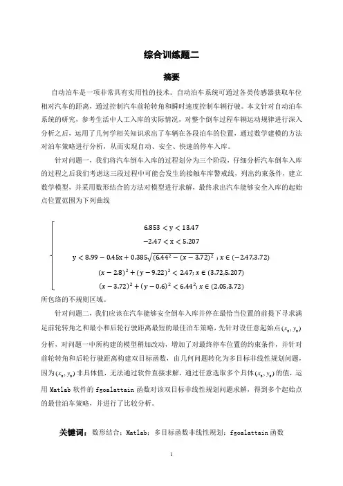
综合训练题二摘要自动泊车是一项非常具有实用性的技术。

自动泊车系统可通过各类传感器获取车位相对汽车的距离，通过控制汽车前轮转角和瞬时速度控制车辆行驶。

本文针对自动泊车系统的研究，参考生活中人工入库的实际情况，对整个倒车过程车辆运动规律进行深入分析之后，运用了几何学相关知识求出了车辆在各段泊车的位置，通过数学建模的方法对泊车策略进行分析，从而实现自动、安全、快速的停车入库。

针对问题一，我们将汽车倒车入库的过程划分为三个阶段，仔细分析汽车倒车入库的过程之后我们考虑这三段过程中可能会发生的接触车库警戒线，列出约束条件，建立数学模型，并采用数形结合的方法对模型进行求解，最终求出汽车能够安全入库的起始点位置范围为下列曲线6.853<y <13.47−2.47<x <5.207y <8.99−0.45x +0.385√(6.442−(x −3.72)2 ;x ∈(−2.47,3.72)(x −2.8)2+(y −9.22)2<2.47;x ∈(3.72,5.207)(x −3.72)2+(y −0.6)2<6.442;x ∈(2.05,3.72)所包络的不规则区域。

针对问题二，我们应该在汽车能够安全倒车入库并停在最恰当位置的前提下寻求满足前轮转角之和最小和后轮行驶距离最短的最佳泊车策略，先针对设任意起始点00(,)x y 分析，对问题一中所构建的模型稍加改动，增加了对最终停车位置的约束条件，并针对前轮转角和后轮行驶距离构建双目标函数，由几何问题转化为多目标非线性规划问题，因为00(,)x y 非具体值，无法通过软件直接求解，通过任意选取多个具体00(,)x y 的值，运用Matlab 软件的fgoalattain 函数对该双目标非线性规划问题求解，得到多个起始点的最佳泊车策略，并进行了比较分析。

关键词：数形结合；Matlab ；多目标函数非线性规划；fgoalattain 函数一、问题重述随着汽车产业及科技的高速发展，智能驾驶汽车成为了国内外公认的未来汽车重要发展方向之一。

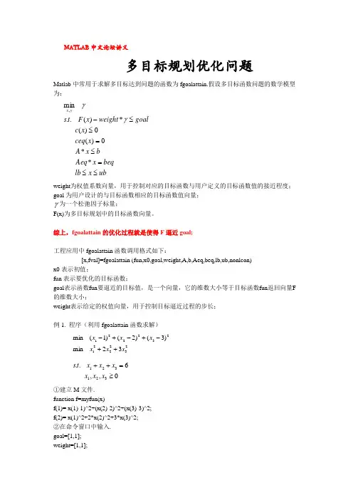
MATLAB 中文论坛讲义多目标规划优化问题Matlab 中常用于求解多目标达到问题的函数为fgoalattain.假设多目标函数问题的数学模型为：ubx lb beqx Aeq bx A x ceq x c goalweight x F t s yx ≤≤=≤=≤≤-**0)(0)(*)(..min ,γγ weight 为权值系数向量，用于控制对应的目标函数与用户定义的目标函数值的接近程度； goal 为用户设计的与目标函数相应的目标函数值向量；γ为一个松弛因子标量；F(x)为多目标规划中的目标函数向量。

综上，fgoalattain 的优化过程就是使得F 逼近goal;工程应用中fgoalattain 函数调用格式如下：[x,fval]=fgoalattain (fun,x0,goal,weight,A,b,Aeq,beq,lb,ub,nonlcon)x0表示初值；fun 表示要优化的目标函数；goal 表示函数fun 要逼近的目标值，是一个向量，它的维数大小等于目标函数fun 返回向量F 的维数大小；weight 表示给定的权值向量，用于控制目标逼近过程的步长；例1. 程序（利用fgoalattain 函数求解）23222123222132min )3()2()1(min x x x x x x ++-+-+-0,,6..321321≥=++x x x x x x t s①建立M 文件.function f=myfun(x)f(1)= x(1)-1)^2+(x(2)-2)^2+(x(3)-3)^2;f(2)= x(1)^2+2*x(2)^2+3*x(3)^2;②在命令窗口中输入.goal=[1,1];weight=[1,1];Aeq=[1,1,1];beq=[6];x0=[1;1;1];lb=[0,0,0]; %也可以写lb=zero(3,1);[x,fval]=fgoalattain(‘myfun’,x0,goal,weight,[ ],[ ],Aeq,beq,lb,[ ])③得到结果.x =3.27271.63641.0909fval =8.9422 19.6364例2.某钢铁公司因生产需要欲采购一批钢材，市面上的钢材有两种规格，第1种规格的单价为3500元/t ，第2种规格的单价为4000元/t.要求购买钢材的总费用不超过1000万元，够得钢材总量不少于2000t.问如何确定最好的采购方案，使购买钢材的总费用最小且购买的总量最多.解：设采购第1、2种规格的钢材数量分别为1x 和2x .根据题意建立如下多目标优化问题的数学模型.0,200010000040003500max 40003500)(min212121211≥≥+≤++=x x x x x x x x x f ①建立M 文件. 在Matlab 编辑窗口中输入：function f=myfun(x)f(1)= 3500*x(1)+4000*x(2);f(2)=-x(1)-x(2);②在命令窗口中输入.goal=[10000000,-2000];weight=[10000000,-2000];x0=[1000,1000];A=[3500,4000;-1,-1];b=[10000000;-2000];lb=[0,0]; %也可以写lb=zero(3,1);[x,fval]=fgoalattain(‘myfun ’,x0,goal,weight,A,b,[ ],[ ],lb,[ ])③得到结果.x =1000 1000fval =7500000 -2000。

优化与决策——多目标线性规划的若干解法及MATLAB 实现摘要：求解多目标线性规划的基本思想大都是将多目标问题转化为单目标规划，本文介绍了理想点法、线性加权和法、最大最小法、目标规划法，然后给出多目标线性规划的模糊数学解法，最后举例进行说明，并用Matlab 软件加以实现。

关键词：多目标线性规划 Matlab 模糊数学。

注：本文仅供参考，如有疑问，还望指正。

一．引言多目标线性规划是多目标最优化理论的重要组成部分，由于多个目标之间的矛盾性和不可公度性,要求使所有目标均达到最优解是不可能的,因此多目标规划问题往往只是求其有效解(非劣解)。

目前求解多目标线性规划问题有效解的方法,有理想点法、线性加权和法、最大最小法、目标规划法。

本文也给出多目标线性规划的模糊数学解法。

二．多目标线性规划模型多目标线性规划有着两个和两个以上的目标函数,且目标函数和约束条件全是线性函数,其数学模型表示为：11111221221122221122max n n n nr r r rn nz c x c x c x z c x c x c x z c x c x c x =+++⎧⎪=+++⎪⎨ ⎪⎪=+++⎩ （1）约束条件为：1111221121122222112212,,,0n n n n m m mn n mn a x a x a x b a x a x a x b a x a x a x bx x x +++≤⎧⎪+++≤⎪⎪ ⎨⎪+++≤⎪≥⎪⎩ （2） 若（1）式中只有一个1122i i i in n z c x c x c x =+++ ，则该问题为典型的单目标线性规划。

我们记:()ij m n A a ⨯=,()ij r n C c ⨯=,12(,,,)T m b b b b = ,12(,,,)T n x x x x = ，12(,,,)T r Z Z Z Z = .则上述多目标线性规划可用矩阵形式表示为:max Z Cx =约束条件：0Ax bx ≤⎧⎨≥⎩（3）三．MATLAB 优化工具箱常用函数[3]在MA TLAB 软件中，有几个专门求解最优化问题的函数，如求线性规划问题的linprog 、求有约束非线性函数的fmincon 、求最大最小化问题的fminimax 、求多目标达到问题的fgoalattain 等,它们的调用形式分别为：①.[x,fval]=linprog(f,A,b,Aeq,beq,lb,ub)f 为目标函数系数,A,b 为不等式约束的系数, Aeq,beq 为等式约束系数, lb,ub 为x 的下限和上限, fval 求解的x 所对应的值。

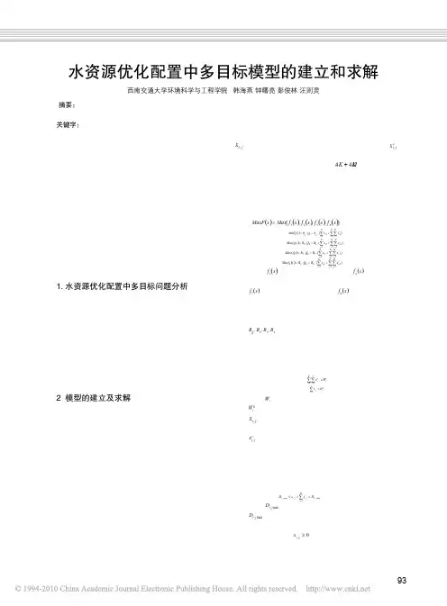
93河南科技2010.2下水资源优化配置是指在流域或特定的区域范围内，运用系统工程理论和优化方法，以水资源的可持续利用和经济社会的可持续发展为目标，遵循公平、高效、统筹兼顾和可持续利用的原则，采取除害与兴利、水量与水质、开源与节流、工程与非工程措施相结合的方法，通过合理抑制需求、有效增加供水、积极保护生态环境等手段和措施，对多种可利用水资源在区域间和各用水部门间进行最优化调配和分配，力求水资源与其他资源合理配置，实现有限水资源的经济、社会和生态环境综合效益最大[1]。

水资源的优化配置研究可为水量和水质在时间和空间上的合理调配和使用以及保障水资源的可持续利用提供科学依据和对策、措施。

因此，水资源的优化配置研究在解决我国的水资源问题，实现水资源的可持续利用等方面均占有重要地位，对促进经济社会的可持续发展具有重要理论和实际意义。

1. 水资源优化配置中多目标问题分析区域水资源系统往往是一个用水部门众多的大系统，在现代水资源优化配置思路中，己经改变了过去以经济效益为中心的基本观念，不仅仅是要获得尽可能大的经济效益，还必须将生态环境保护放到重要位置，同时要兼顾引水保障和粮食安全的问题。

配置中所考虑的不同问题可以作为不同的目标，各个目标之间相互矛盾而又不可公度，这就使得区域水资源优化配置转变成一个多目标优化的问题，在协调各个配置目标时要以公平与高效为基本分配原则，目标是寻求水量在各个用水部门之间的最优分配，实现水资源利用的可持续发展。

2 模型的建立及求解2. 1水资源多目标优化配置模型的建立2. 1.1 决策变量根据区域的地形地貌、水利条件、行政区划，一般可将区域划分为若干分区。

根据各水源在区内的配水特性，可将水源划分成两类:共用水源和独立水源。

所谓共用水源是指能同时向两个或两个以上的分区供水的水源。

独立水源是指只能给水源所在的分区供水的水源。

本研究假设区域划分为K个分区，i =1，2，…，K，本文将k分区内所有独立水源计为1个水源、分别有J(K)个用水部门j=1,2, …，J(K)（本文各区均定为4个，分别为工业、生活、农业、生态）。

§18. 运用目标达到法求解多目标规划用目标达到法求解多目标规划的计算过程，可以通过调用Matlab软件系统优化工具箱中的fgoalattain函数实现。

在Matlab的优化工具箱中，fgoalattain函数用于解决此类问题。

其数学模型形式为：minγF(x)-weight ·γ≤goalc(x) ≤0ceq(x)=0A x≤bAeq x=beqlb≤x≤ub其中，x，weight，goal，b，beq，lb和ub为向量；A和Aeq为矩阵；c(x)，ceq(x)和F(x)为函数。

调用格式：x=fgoalattain(F,x0,goal,weight)x=fgoalattain(F,x0,goal,weight,A,b)x=fgoalattain(F,x0,goal,weight,A,b,Aeq,beq)134x=fgoalattain(F,x0,goal,weight,A,b,Aeq,beq,lb,ub)x=fgoalattain(F,x0,goal,weight,A,b,Aeq,beq,lb,ub,nonlcon)x=fgoalattain(F,x0,goal,weight,A,b,Aeq,beq,lb,ub,nonlcon,options)x=fgoalattain(F,x0,goal,weight,A,b,Aeq,beq,lb,ub,nonlcon,options,P1,P2)[x,fval]=fgoalattain(…)[x,fval,attainfactor]=fgoalattain(…)[x,fval,attainfactor,exitflag,output]=fgoalattain(…)[x,fval,attainfactor,exitflag,output,lambda]=fgoalattain(…)说明：F为目标函数；x0为初值；goal为F达到的指定目标；weight为参数指定权重；A、b为线性不等式约束的矩阵与向量；Aeq、beq为等式约束的矩阵与向量；lb、ub为变量x的上、下界向量；nonlcon为定义非线性不等式约束函数c(x)和等式约束函数ceq(x)；options中设置优化参数。