powerpoint模板-gaussian

高斯模板计算方法English:The Gaussian template refers to a method used to smooth out images and reduce noise while preserving the edges of the objects in the image. The template is a 2D distribution that is defined by the Gaussian function, which is a bell-shaped curve. The method involves convolving the image with this Gaussian template, which means that each pixel in the image is combined with its neighboring pixels based on their weights determined by the Gaussian function. This process results in the blurring of the image, with the degree of blurring determined by the standard deviation of the Gaussian function. A larger standard deviation value leads to a greater blurring effect. The Gaussian template is commonly used in image processing tasks such as edge detection, image enhancement, and noise reduction.中文翻译:高斯模板是一种用于平滑图像、减少噪音并保留图像中物体边缘的方法。

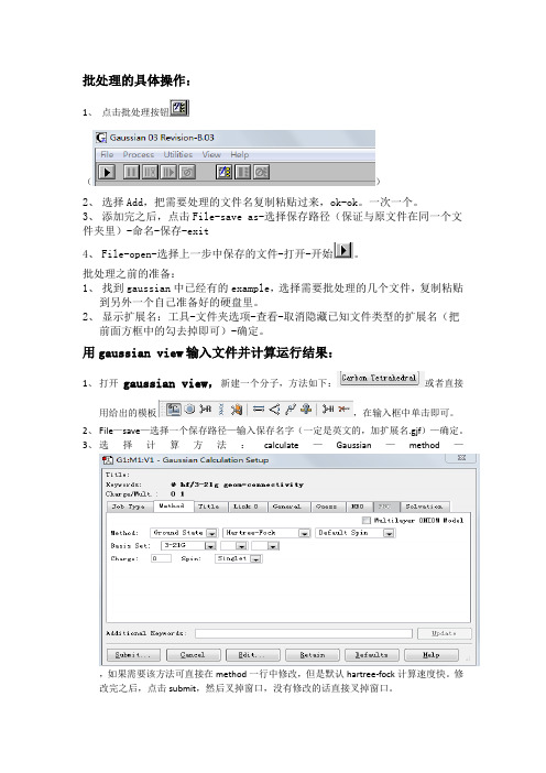
批处理的具体操作：
1、点击批处理按钮
（）
2、选择Add，把需要处理的文件名复制粘贴过来，ok-ok。

一次一个。

3、添加完之后，点击File-save as-选择保存路径（保证与原文件在同一个文件夹里）-命名-保存-exit
4、File-open-选择上一步中保存的文件-打开-开始。

批处理之前的准备：
1、找到gaussian中已经有的example，选择需要批处理的几个文件，复制粘贴
到另外一个自己准备好的硬盘里。

2、显示扩展名：工具-文件夹选项-查看-取消隐藏已知文件类型的扩展名（把
前面方框中的勾去掉即可）-确定。

用gaussian view输入文件并计算运行结果：
1、打开gaussian view，新建一个分子，方法如下：或者直接
用给出的模板，在输入框中单击即可。

2、File—save—选择一个保存路径—输入保存名字（一定是英文的，加扩展名.gjf）—确定。

3、选择计算方法：calculate—Gaussian—method—
，如果需要该方法可直接在method一行中修改，但是默认hartree-fock计算速度快。

修改完之后，点击submit，然后叉掉窗口，没有修改的话直接叉掉窗口。

4、打开刚才保存的文件，对其中的内容进行修改：
，第四行中的改为
opt，把这些东西删掉，之后敲回车键几下，保存文件。

5、打开gaussian，file—open—选择刚刚保存的文件，打开后，点击对话框中的ok，再点击
开始，这时会提示你保存的输出结果，点确定，点开始按钮运行。

（一）目标生成一个（2n+1）×（2n+1）大小的高斯模板h（标准为sigma），然后用此模板对图像进行滤波。

具体要求注：这里采用了多种方法：方法一：自己编写高斯模板，并用imfilter等函数。

方法二：自己编写高斯模板，不能用imfilter等函数。

方法三：利用matlab中的 fspecial 来产生高斯模板。

（二）前言为什么要讨论上述方法呢？通过编程显示便可知道方法的不同产生的高斯函数会略有不同。

编程前，我们首先应该了解一下高斯函数及高斯滤波。

（三）相关知识1.高斯函数的定义根据一维高斯函数，可以推导得到二维高斯函数：参考博文：高斯函数以及在图像处理中的应用总结2.高斯滤波原理高斯滤波就是对整幅图像进行加权平均的过程，每一个像素点的值，都由其本身和邻域内的其他像素值经过加权平均后得到。

高斯滤波的具体操作是：用一个模板（或称卷积、掩模）扫描图像中的每一个像素，用模板确定的邻域内像素的加权平均灰度值去替代模板中心像素点的值。

3.高斯模板公式二维高斯模板可以通过矩阵m来实现，假设模板的大小为（2k+1, 2k+1）, 其中k为模板中心，则m（i，j）的值如下所示：4.模板与图像滤波的实现（实质：卷积）其中，w表示高斯算子，a，b表示算子大小。

（四）不同方法实现高斯模板的区别这里先放结果，代码部分见方法一由于不同标准差会造成不同效果，编程代码见附录2，这里显示我以0.5：0.5：4.5的sigma来设计不同的15*15高斯低通模板显示不同高斯模板之间的区别，如下所示：下面为我根据高斯函数表达书编写的高斯模板三维显示图：matlab中自带高斯模板函数，显示如下：由上述可知，sigma越小，函数越窄越高，与前述的理论不同。

高斯模板与自己编写的区别主要是在模板中心值的不同，中心像素值的不同会导致周围的值也有所不同，运行方法一中代码你就知道了，这里我就不放了。

（五）实现过程与结果1.方法1实验结果如下所示：自己编写的滤波效果：matlab自带对比如下：（左边自己，后边matlab)实验代码：n_size =15;center_n =(n_size +1)/2;n_row = n_size;n_col = n_size;array_sigma =0.5:0.5:4.5;map_x =1:n_row; map_y =1:n_col;figure('name','不同高斯模板三维图')for k =1:9sigma =array_sigma(k);fori=1: n_rowforj=1: n_coldistance_s =double((i-center_n-1)^2+(j-center_n-1)^2);g_ry(i,j)=exp((-1)* distance_s/(2*sigma^2))/(2*pi*(sigma^2));endenddisp(num2str(sigma));disp(g_ry)subplot(3,3,k);surf(map_x,map_y,g_ry);title(num2str(sigma));endfigure('name','matlab不同高斯模板三维图')for k =1:9sigma =array_sigma(k);gausfilter =fspecial('gaussian',[n_row n_col],sigma);disp(num2str(sigma));disp(gausfilter)subplot(3,3,k);surf(map_x,map_y,g_ry);tit le(num2str(sigma));endfigure('name','不同高斯模板滤波效果(my)')srcimg =imread('pic_3_x2.jpg');subplot(3,4,1);imshow(uint8(srcimg));title('原图');grayimg =rgb2gray(srcimg);subplot(3,4,5);imshow(uint8(grayimg));title('灰度图');image_noise =imnoise(grayimg,'gaussian');subplot(3,4,9);imshow(uint8(image_noise));title('加噪图');for k =1:9sigma =array_sigma(k);fori=1: n_rowforj=1: n_coldistance_s =double((i-center_n-1)^2+(j-center_n-1)^2);g_ry(i,j)=exp((-1)* distance_s/(2*sigma^2))/(2*pi*(sigma^2));endendsubplot(3,4,k+ceil(k/3));gry_img=imfilter(image_noise,g_ry);imshow(gry_img);title(num2str(sigma));endfigure('name','不同高斯模板滤波效果(matlab)')subplot(3,4,1);imshow(uint8(srcimg));title('原图');subplot(3,4,5);imshow(uint8(grayimg));title('灰度图');subplot(3,4,9);imshow(uint8(image_noise));title('加噪图');for k =1:9sigma =array_sigma(k);gausfilter =fspecial('gaussian',[n_row n_col],sigma);subplot(3,4,k+ceil(k/3));gry_img =imfilter(image_noise,gausfilter);imshow(gry_img);title(num2str(sigma));end2.方法2实验结果如下：实验代码：srcimg=imread('pic_3_x2.jpg');grayimg=rgb2gray(uint8(srcimg));k =size(grayimg);[grayimg_row,grayimg_col]=size(grayimg);sigma =1.6;n =7;n_row =2*n+1;n_col =2*n+1;image_noise =imnoise(grayimg,'gaussian');g_ry =[];fori=1:n_rowforj=1:n_coldistance_s=double((i-n-1)^2+(j-n-1)^2);g_ry(i,j)=exp(-distance_s/(2*sigma*sigma))/(2*pi*sigma*sigma);endendg_ry=g_ry/sum(g_ry(:));dstimg_gry =zeros(grayimg_row,grayimg_col);fori=1:grayimg_rowforj=1:grayimg_coldstimg_gry(i,j)=image_noise(i,j);endendtemp=[];for ai=n+1:grayimg_row-n-1for aj=n+1:grayimg_col-n-1temp=0;for bi=1:n_rowfor bj=1:n_coltemp= temp+(dstimg_gry(ai+bi-n-1,aj+bj-n-1)*g_ry(bi,bj));endenddstimg_gry(ai,aj)=temp;endenddstimg_gry=uint8(dstimg_gry);gausfilter =fspecial('gaussian',[n_row n_col],sigma);gmf_img=imfilter(image_noise,gausfilter,'conv');figure('name','不处理边界的高斯滤波对比')subplot(2,2,1);imshow(grayimg);title('原图');subplot(2,2,2);imshow(image_noise);title('噪声图');subplot(2,2,3);imshow(dstimg_gry);title('my高斯滤波');subplot(2,2,4);imshow(gmf_img);title('matlab高斯滤波');方法2和方法3可参考matlab实现图像滤波——高斯滤波【这篇博文】3.方法3实验结果：实验代码：srcimg=imread('pic_3_x2.jpg');grayimg=rgb2gray(uint8(srcimg));[grayimg_row,grayimg_col]=size(grayimg);sigma =1.6;n =7;n_row =2*n+1;n_col =2*n+1;image_noise =imnoise(grayimg,'gaussian');g_ry =[];fori=1:n_rowforj=1:n_coldistance_s=double((i-n-1)^2+(j-n-1)^2);g_ry(i,j)=exp(-distance_s/(2*sigma*sigma))/(2*pi*sigma*sigma);endendg_ry=g_ry/sum(g_ry(:));dstimg_gry =zeros(grayimg_row,grayimg_col);midimg=zeros(grayimg_row+2*n,grayimg_col+2*n);fori=1:grayimg_rowforj=1:grayimg_colmidimg(i+n,j+n)=image_noise(i,j);endenddstimg_ry=zeros(grayimg_row,grayimg_col);temp=[];for ai=n+1:grayimg_row+nfor aj=n+1:grayimg_col+ntemp_row=ai-n;temp_col=aj-n;temp=0;for bi=1:n_rowfor bj=1:n_rowtemp= temp+(midimg(temp_row+bi-1,temp_col+bj-1)*g_ry(bi,bj));endenddstimg_ry(temp_row,temp_col)=temp;endenddstimg_ry=uint8(dstimg_ry);gausfilter =fspecial('gaussian',[n_row n_col],sigma);gmf_img=imfilter(image_noise,gausfilter,'conv');figure('name','高斯滤波对比')subplot(2,2,1);imshow(grayimg);title('原图');subplot(2,2,2);imshow(image_noise);title('噪声图');subplot(2,2,3);imshow(dstimg_ry);title('my高斯滤波');subplot(2,2,4);imshow(gmf_img);title('matlab高斯滤波');。

频域滤波模板
常见的频域滤波模板包括：
1. 高通滤波器（High-Pass Filter）：能够滤除低频信号，只保
留高频信号。

适用于去除图像中的低频噪声、模糊和平滑等，同时保留边缘和细节信息。

常见的高通滤波器包括Butterworth、Gaussian、Laplacian等。

2. 低通滤波器（Low-Pass Filter）：能够滤除高频信号，只保
留低频信号。

适用于去除图像中的高频噪声、平滑等，常见的低通滤波器包括Butterworth、Gaussian、Mean、Median等。

3. 带通滤波器（Band-Pass Filter）：只保留选定的频带信号，
去除其他频率信号。

适用于去除一定频率范围内的噪声和干扰，在物体检测、医学影像处理等方面有着广泛的应用。

常见的带通滤波器包括IIR、FIR等。

4. 带阻滤波器（Band-Stop Filter）：只滤除选定的频带信号，
保留其他频带信号。

适用于去除某些频率范围内的干扰和噪声。

常见的带阻滤波器包括IIR、FIR等。

5. 频率加突滤波器（Frequency Notch Filter）：用于去除特定
的频率干扰，保留其他频率信号，用于解决丢失或偏移频率问题。

数字图像处理-频域滤波-⾼通低通滤波频域滤波频域滤波是在频率域对图像做处理的⼀种⽅法。

步骤如下：滤波器⼤⼩和频谱⼤⼩相同，相乘即可得到新的频谱。

滤波后结果显⽰，低通滤波去掉了⾼频信息，即细节信息，留下的低频信息代表了概貌。

常⽤的例⼦，⽐如美图秀秀的磨⽪，去掉了脸部细节信息（痘坑，痘印，暗斑等）。

⾼通滤波则相反。

⾼通/低通滤波1.理想的⾼/低通滤波顾名思义，⾼通滤波器为：让⾼频信息通过，过滤低频信息；低通滤波相反。

理想的低通滤波器模板为：其中，D0表⽰通带半径，D(u，v)是到频谱中⼼的距离（欧式距离），计算公式如下：M和N表⽰频谱图像的⼤⼩，（M/2，N/2）即为频谱中⼼理想的⾼通滤波器与此相反，1减去低通滤波模板即可。

部分代码：# 定义函数，显⽰滤波器模板def showTemplate(template):temp = np.uint8(template*255)cv2.imshow('Template', temp)return# 定义函数，显⽰滤波函数def showFunction(template):row, col = template.shaperow = np.uint16(row/2)col = np.uint16(col/2)y = template[row, col:]x = np.arange(len(y))plt.plot(x, y, 'b-', linewidth=2)plt.axis([0, len(x), -0.2, 1.2])plt.show()return# 定义函数，理想的低通/⾼通滤波模板def Ideal(src, d0, ftype):template = np.zeros(src.shape, dtype=np.float32) # 构建滤波器 r, c = src.shapefor i in range(r):for j in range(c):distance = np.sqrt((i - r/2)**2 + (j - c/2)**2)if distance < d0:template[i, j] = 1else:template[i, j] = 0if ftype == 'high':template = 1 - templatereturn templateIdeal2. Butterworth⾼/低通滤波Butterworth低通滤波器函数为：从函数图上看，更圆滑，⽤幂系数n可以改变滤波器的形状。