《统计学—基于SPSS》((06)第6章 假设检验(S3)
- 格式:pptx
- 大小:1.69 MB
- 文档页数:89

SPSS假设检验1. 简介SPSS(Statistical Package for the Social Sciences)是一种非常常用的统计软件,被广泛应用于社会科学研究中。
其中,假设检验是SPSS中常用的统计方法之一,用于验证研究者对总体或样本的某种假设。
2. 假设检验的概念假设检验是统计学中的一种重要方法,用于判断一个统计推断是否与样本数据一致。
在假设检验中,通常会提出一个原假设(H0)和一个备择假设(H1),然后根据样本数据对两个假设进行检验,以确定是否拒绝原假设,从而对总体进行推断。
3. SPSS中的假设检验SPSS中提供了丰富的假设检验方法,涵盖了多种统计推断的情况。
下面将介绍几种常见的假设检验方法。
3.1 单样本 t 检验单样本 t 检验用于判断一个样本的均值是否与一个已知的常数有显著性差异。
在SPSS中,进行单样本 t 检验的步骤如下:1.导入数据:在SPSS中打开或导入数据文件。
2.选择变量:选择要进行 t 检验的变量。
3.进行检验:选择菜单栏上的“分析”-“比较均值”-“单样本 t 检验”。
4.设置参数:选择相关的变量和检验参数,点击“确定”进行分析。
5.查看结果:SPSS将显示 t 检验的结果,包括均值、标准差、t 值、自由度和显著性等。
3.2 独立样本 t 检验独立样本 t 检验用于判断两个独立样本的均值是否存在显著性差异。
在SPSS中,进行独立样本 t 检验的步骤如下:1.导入数据:在SPSS中打开或导入数据文件。
2.选择变量:选择需要进行对比的两个变量。
3.进行检验:选择菜单栏上的“分析”-“比较均值”-“独立样本 t 检验”。
4.设置参数:选择相关的变量和检验参数,点击“确定”进行分析。
5.查看结果:SPSS将显示独立样本 t 检验的结果,包括均值、标准差、t 值、自由度和显著性等。
3.3 配对样本 t 检验配对样本 t 检验用于判断同一组个体在两个不同时间点或条件下的均值是否存在显著性差异。

SPSS假设检验实验⽬的::实验⽬的1、学会使⽤SPSS的简单操作。
2、掌握假设检验。
:实验内容:实验内容1.⼀个总体均值的检验(⼩样本);2.两个总体均值之差的检验;3.绘制正态概率图;4.S—W检验。
实验步骤: 1.⼀个总体均值的检验(⼩样本):单总体的Z检验和t检验。
设是取⾃正态总体的⼀个样本,要检验。
其中为已知的常数。
为了说明如何构造检验统计量和拒绝域,先看⼀个简单的情形。
设总体⽅差是已知的,记为,设为样本均值,则。
设为真,即,对作标准化,得到上述的Z就是要构造的检验统计量。
设定显著性⽔平为0.05,因为,的概率为0.05,所以检验的拒绝域是。
如果由样本计算得到,与⼩概率原理⽭盾,从⽽拒绝原假设。
在实际应⽤中,总体的⽅差是未知的。
因⽽需要样本⽅差代替总体⽅差,相应地,检验统计量编程了t统计量。
设与分别为样本的均值和样本⽅差,当为真时,可知统计量对于给定的显著性⽔平,检验的拒绝域是。
其中临界值满⾜条件。
它就是⾃由度为(N-1)的t分布的双侧分为点。
如果由样本观测值代⼊,计算得到的t值满⾜,则拒绝原假设。
SPSS检验结果不给出临界值,⽽是在给出t值的同时给出它的显著性概率(也成为p值或相伴概率,记为p或Sig)。
计算⼀个双侧检验问题,SPSS操作如下:“分析”→“⽐较均值”→“单样本T检验”,在打开的对话框中填好“检验变量”列表框和“检验值”⽂本框。
单击“确定”。
输出结果中的Sig.(双侧)就是p值。
⽐较p值与检验⽔准。
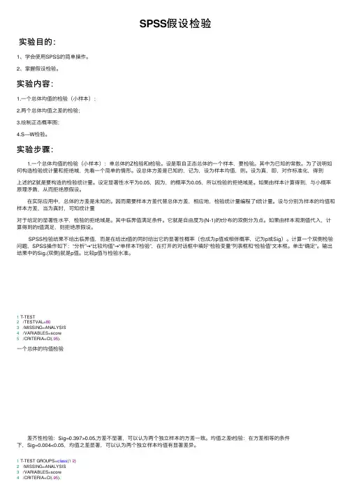
1 T-TEST2 /TESTVAL=803 /MISSING=ANALYSIS4 /VARIABLES=score5 /CRITERIA=CI(.95).⼀个总体的均值检验 差齐性检验:Sig=0.397>0.05,⽅差不显著,可以认为两个独⽴样本的⽅差⼀致。
均值之差t检验:在⽅差相等的条件下,Sig=0.004<0.05,均值之差显著,可以认为两个独⽴样本均值有显著差异。
SPSS数据统计分析与实践主讲:周涛副教授北京师范大学资源学院2007 -10 -16教学网站:/Courses/SPSS第六章假设检验(Hypothesis Testing)本章内容:一、单样本假设检验z基本统计原理z SPSS应用实例二、独立双样本假设检验z基本原理z SPSS应用实例三、配对双样本假设检验z基本原理z SPSS应用实例几个基本常识z统计分析常常采取抽样的研究方法。
即从总体中抽取一定数量的样本进行研究来推论总体的特征。
z由于总体中的每个个体间存在差异,即使严格遵守随机抽样原则也会有样本统计量与总体参数之间有所不同。
z实验者测量技术的差别或测量仪器精确程度的差别等也会造成一定的偏差,使样本统计量与总体参数之间存在差异。
几个基本常识Cont. z均值不相等的两个样本不一定来自均值不同的总体?(从均值相等的总体等抽样的均值可能不相等,这是抽样造成的)z两个样本的均值不同,其差异是否具有统计意义,能否说明总体差异?(只有样本均值的差异具有统计意义时,才能推断总体均值有差异)z校验假设的基本思想是统计学的“小概率反证法”一、单样本假设检验z基本统计原理z SPSS应用实例单样本假设检验的用途z The goal in a one-sample t test is to test if the mean ofa single sample differs from a hypothesized populationvalue.z e.g. You read that in the U.S., the average IQ is 100and you know that the average IQ for your coworkers is127.5. Are you coworkers smarter than the averageperson in the U.S.?z To answer this type of question in SPSS, request a one-sample t test to compare the mean of the sample IQvalue with the constant 100.单样本假设检验的基本统计原理主要内容:•Hypothesis Testing Methodology (假设检验的方法论)•Z Test for the Mean (σ Known) (Z检验方法,σ已知)•p-Value Approach to Hypothesis Testing(P-值检验方法)•t Test of Hypothesis for the Mean (t检验方法)z A hypothesis is an assumption about the population parameter.z A parameter is a Populationmean or proportionz The parameter must beidentified before analysis.I assume the mean GPA(总平均成绩) of this class is 3.5!What is a Hypothesis?The Null Hypothesis (零假设),H0z States the Assumption (numerical) to be testede.g. The average # TV sets in US homes is atleast 3(H: µ ≥3)z Begin with the assumption that the nullhypothesis is TRUE.(Similar to the notion of innocent until proven guilty)•Refers to the Status Quo (现状)•Always contains the‘= ‘sign•The Null Hypothesis may or may not be rejected.z Is the opposite of the null hypothesise.g. The average # TV sets in US homes isless than 3(H 1: µ< 3)z Challenges the Status Quo (现状)z Never contains the ‘=‘signz The Alternative Hypothesis may or may not be accepted The Alternative Hypothesis (备择假设),H 1Identify the ProblemSteps:z State the Null Hypothesis (H0: µ≥3)z State its opposite, the Alternative: µ< 3)Hypothesis (H1z Hypotheses are mutually exclusive (互斥的)&exhaustive(无遗漏的)z Sometimes it is easier to form thealternative hypothesis first.PopulationAssume the populationmean age is 50.(Null Hypothesis)REJECT The Sample Mean Is 20SampleNull Hypothesis50?20=≅=µX Is Hypothesis Testing ProcessNo, not likely!Sample Meanµ= 50Sampling DistributionIt is unlikely that we would get a sample mean of this value ...... if in fact this were the population mean.... Therefore, we reject the null hypothesis thatµ= 50.20H 0Reason for Rejecting H 0zDefines Unlikely Values of Sample Statistic if Null Hypothesis Is TruezCalled Rejection Region of Sampling DistributionzDesignated α(alpha)zTypical values are 0.01, 0.05, 0.10z Selected by the Researcher at the Start zProvides the Critical Value(s)of the TestLevel of Significance,α(临界值)Level of Significance,α and the Rejection RegionH 0:µ≥3 H 1: µ< 30H 0: µ≤3 H 1: µ> 3H 0: µ= 3 H 1: µ≠3ααα/2Critical Value(s)Rejection RegionsErrors in Making Decisionsz Type I Errorz Reject True Null Hypothesisz Has Serious Consequencesz Probability of Type I Error Isαz Called Level of Significance(显著性水平)z Type II Errorz Do Not Reject False Null Hypothesis(没有拒绝错误的零假设)z Probability of Type II Error Is β(Beta)α &β Have anInverse RelationshipReduce probability of one errorand the other one goes up.βαzConvert Sample Statistic (e.g., ) to Standardized Z VariablezCompare to Critical Z Value(s)zIf Z test Statistic falls in Critical Region , Reject H 0; Otherwise Do Not Reject H 0Z-Test Statistics (σ Known)Test StatisticX nX X Z XXσµσµ−=−=p Value Testz Probability of Obtaining a Test Statistic More Extreme than Actual Sample Value Given H0 Is Truez Called Observed Level of Significancez Smallest Value of a H0Can Be Rejectedz Used to Make Rejection Decisionz If p value ≥α,Do Not Reject H0z If p value <α, Reject H01.State H 0H 0:µ ≥32.State H 1H 1: µ < 33.Choose αα= .054.Choose n n = 1005.Choose Test:Z Test (or p Value)Hypothesis Testing: StepsTest the Assumption that the true mean # ofTV sets in US homes is at least 3.6. Set Up Critical Value(s)Z = -1.6457. Collect Data100 households surveyed 8. Compute Test Statistic Computed Test Stat.= -29. Make Statistical Decision Reject Null Hypothesis10. Express DecisionThe true mean # of TV set is less than 3 in the US households.Hypothesis Testing: StepsTest the Assumption that the average # ofTV sets in US homes is at least 3.(continued)zAssumptionsz Population is normally distributedz If not normal , only slightly skewed & a large sample taken zParametric test procedurezt test statistict-Test: σ UnknownnSX t µ−=Example: One Tail t-TestA random sample of 36boxes showed X = 372.5, and S =15. Test at the α=0.01level.368 gm.H 0: µ ≤368 H 1: µ >368σ is not given,Does an average box of cereal contain more than 368grams of cereal?z α = 0.01z n = 36, df= 35z Critical Value: 2.4377Test Statistic:Decision:Conclusion:Do Not Reject at α = .01No Evidence that True Mean Is More than 368Z02.4377.01Reject Example Solution: One TailH 0: µ ≤368 H 1: µ >36880.136153685.372=−=−=nSX t µSPSS单样本T检验实例SPSS单样本T检验实例A manufacturer of high-performance automobiles produces discbrakes (盘式制动器)that must measure 322 millimeters(毫米)in diameter. Quality control randomly draws 16 discs made by each of eight production machines(总计128个观测量)and measures their diameters.Use One Sample T Test to determine whether or not the mean diameters of the brakes in each sample significantly differ from 322 millimeters.A nominal variable, Machine Number, identifies the productionmachine used to make the disc brake. Because the data from each machine must be tested as a separate sample, the file must first be split into groups by Machine Number.数据文件:brakes.sav操作步骤1. 以变量“Machine Number”分割文件操作步骤2. 调用“One-Sample T Test”过程操作步骤3. 在One-Sample T Test的主对话框中输入要检验的变量,并输入要检验的值(322),并在“Options”中设置置信区间(90%)操作步骤4. 对输出结果进行解释One-Sample Test-.53315.602-.0014858-.006375.0034045.33615.000.0142629.009577.018948-.65515.522-.0017174-.006311.002876-2.61315.020-.0045649-.007628-.0015021.84715.085.0042486.000216.0082821.13415.274.0024516-.001337.0062402.65015.018.0061813.002092.010270-1.71315.107-.0033014-.006680.000077Disc Brake Diameter (mm)Disc Brake Diameter (mm)Disc Brake Diameter (mm)Disc Brake Diameter (mm)Disc Brake Diameter (mm)Disc Brake Diameter (mm)Disc Brake Diameter (mm)Disc Brake Diameter (mm)Machine Number 12345678tdfSig. (2-tailed)Mean Difference Lower Upper 90% Confidence Interval of the Difference Test Value = 3221. The columnlabeled Sig. (2-tailed)displays a probability from the t distribution with 15 degrees of freedom.2.The 90%Confidence Interval of the Differenceprovides an estimate of the boundaries between which the true mean difference lies in 90% of all possible random samples of 16 disc brakes produced by this machine.3. Since their confidence intervals lie entirely above 0.0, you can safely say that machines 2, 5and 7are producing discs that are significantly wider than 322mm on the average.4. Similarly, because its confidenceinterval lies entirely below 0.0, machine 4is producing discs that are not wide enough .二、独立双样本假设检验z基本原理z SPSS应用实例独立双样本假设检验—基本原理主要内容:Comparing Two Independent Samples (两个独立样本的比较): Z Test for the Difference in Two Means (Z检验方法)t Test for Difference in Two Means (t检验方法)•F Test for Difference in two Variances (方差相等检验,F检验)Independent Samples•Different Data Sources:Unrelated (不相关)Independent (独立)Sample selected from one population has no effector bearing on the sample selected from the otherpopulation.•Use Difference Between the 2 Sample Means •Use Pooled Variance(合并方差)t TestzAssumptions (前提假设):zSamples are Randomly and Independentlydrawnz Data Collected are Numerical z Population Variances Are Known zSamples drawn are LargezTest Statistic:Z Test for Differences in Two Means (Variances Known)2221122121n n )()X X (Z σσµµ+−−−=zAssumptions (前提假设):z Both Populations Are Normally Distributed zOr, If Not Normal, Can Be Approximated byNormal DistributionzSamples are Randomly and IndependentlydrawnzPopulation Variances Are Unknown ButAssumed Equalt Test for Differences in Two Means (Variances Unknown)Pooled-Variance t Test (Part 1) 1. Setting Up the Hypothesis:H0: µ 1≤µ 2 H1: µ 1> µ 2H0: µ 1-µ 2= 0 H1: µ 1-µ 2 ≠0H0: µ 1= µ 2 H1: µ 1≠µ 2H0: µ 1≥µ 2H0: µ 1-µ 2≤0H1: µ 1-µ 2> 0H0: µ 1-µ 2≥0H1: µ 1-µ 2 < 0OROROR LeftTailRightTailTwoTailH1: µ 1< µ 2Pooled-Variance t Test (Part 2)2. Calculate the Pooled Sample Variances as an Estimate of the Common Populations Variance:)n ()n (S )n (S )n (Sp1111212222112−+−−+−=2pS 21S 22S 1n 2n = Pooled-Variance = Variance of Sample 1= Variance of sample 2= Size of Sample 1= Size of Sample 2t X X S n S n S n n df n n P=−−−=−×+−×−+−=+−12122112222121211112µµHypothesizedDifference Pooled-Variance t Test (Part 3)3. Compute the Test Statistic:())(()()()()⎟⎟⎠⎞⎜⎜⎝⎛+•112p S n 1n 2__Pooled-Variance t Test: Examplez You’re a financial analyst for Charles Schwab. Isthere a difference in dividend (股息)yield between stocks listed on the NYSE(纽约证券交易所)& NASDAQ? You collect the following data:NYSE NASDAQNumber2125Mean 3.27 2.53Std Dev 1.30 1.16z Assuming equal variances, isthere a difference in averageyield (α = 0.05)?t X X S n n S n S n S n n PP=−−−=−−==−×+−×−+−=−×+−×−+−=1212212211222212223272530151********11112111302511162112511510µµ.......Calculating the Test Statistic:((((((((((()))))))))))⎟⎟⎠⎞⎜⎜⎝⎛+•11⎟⎟⎠⎞⎜⎜⎝⎛+•11z H 0: µ1 -µ2= 0 (µ1 = µ2)z H 1: µ1 -µ2≠0 (µ1≠µ2)z α = 0.05z df = 21 + 25 -2 = 44z Critical Value(s):Test Statistic:Decision:Conclusion:Reject at a = 0.05There is evidence of a difference in means.t0 2.0154-2.0154.025Reject H 0Reject H 0.025t =−=327253151********....Solution⎟⎟⎠⎞⎜⎜⎝⎛+•11F Test for Differences in Two Variances•The F test Statistic:F == Variance of Sample 1n 1 -1 = degrees of freedomn 2 -1 = degrees of freedomF0 21S 21S 22S 22S = Variance of Sample 2zTests for Differences in 2 Independent Population Variances z Parametric Test Procedure zAssumptionszBoth Populations Are Normally DistributedzTest Is Not Robust to ViolationsF Test for the Difference in Two Population VarianceszHypotheses z H 0:σ12= σ22z H 1: σ12≠σ22zTest Statistic z F = S 12/S 22zTwo Sets of Degrees of Freedom z df 1= n 1-1;df 2= n 2-1zCritical Values:F L ( )and F U ()F L = 1/F U *(* degrees of freedom switched)F Test for the Difference in Two Population VariancesReject H 0Reject H 0α/2α/2Do Not Reject F0F LF Un 1-1, n 2-1n 1 -1 , n 2 -1F Test: An Examplez Assume you are a financial analyst for Charles Schwab. You want to compare dividend yields between stocks listed on the NYSE & NASDAQ. You collect the following data:NYSE NASDAQNumber2125Mean 3.27 2.53Std Dev 1.30 1.16z Is there a difference in thevariances between the NYSE& NASDAQ at the 0.05level?z H 0:σ12= σ22z H 1: σ12≠σ22z α=.05z df 1=20 df 2=24z Critical Value(s):Test Statistic:Decision:Conclusion:Do not reject at a = 0.05There is no evidence of a difference in variances.0F2.330.415.025Reject Reject .025F ===22130116125...F Test: Example Solution21S 22SH 0: σ12≥σ22H 1: σ12< σ22F Test: One TailH 0: σ12≤σ22H 1: σ12> σ22Reject α =.05F0FReject α =.05α= .05F LF UF L =F U 1or (n 2 -1, n 1-1)Degrees of freedom switchedSPSS双独立样本T检验实例SPSS双独立样本T检验z An analyst at a department store(百货公司) wants to evaluate a recent credit card promotion. To this end, 500 cardholders wererandomly selected. Half received an ad promoting a reduced interest rate on purchases made over the next three months, and halfreceived a standard seasonal ad.z Use Independent-Samples T Test to compare the spending of the two groups.操作步骤:1.打开数据文件(creditpromo.sav)2.调用Independent-Samples T Test。


如何在SPSS数据分析报告中进行假设检验?关键信息项:1、假设检验的类型独立样本 t 检验配对样本 t 检验单因素方差分析多因素方差分析卡方检验2、数据准备要求数据的完整性数据的准确性数据的正态性异常值处理3、假设的设定原假设和备择假设的明确表述假设的合理性和基于的理论或经验基础4、检验步骤选择合适的检验方法在 SPSS 中输入数据和执行检验操作解读检验结果5、结果报告内容检验统计量的值自由度p 值效应量(如适用)6、结果的解释和结论根据 p 值做出决策对效应大小的解释结果在研究背景下的意义11 假设检验的类型在 SPSS 数据分析报告中,常见的假设检验类型包括但不限于以下几种:111 独立样本 t 检验用于比较两个独立样本的均值是否存在显著差异。
例如,比较两组不同治疗方法下患者的康复时间。
112 配对样本 t 检验适用于配对数据,即同一组对象在不同条件下或不同时间点的测量值。
比如,比较同一批患者治疗前后的体重变化。
113 单因素方差分析用于检验一个因素的不同水平对因变量的均值是否有显著影响。
例如,研究不同教育程度对收入的影响。
114 多因素方差分析当存在多个因素同时影响因变量时,使用多因素方差分析。
比如,研究教育程度和工作经验对收入的共同影响。
115 卡方检验主要用于检验两个分类变量之间是否存在关联。
例如,分析性别与某种疾病的患病率是否有关。
12 数据准备要求在进行假设检验之前,确保数据满足以下要求:121 数据的完整性数据应包含所需的所有变量和观测值,不允许有缺失值。
若存在缺失值,需要采取适当的方法进行处理,如删除含缺失值的观测、均值插补或多重插补等。
122 数据的准确性对数据进行仔细检查,确保其没有录入错误或异常值。
异常值可能会对假设检验的结果产生较大影响,需要谨慎处理。
123 数据的正态性对于一些基于正态分布假设的检验方法(如 t 检验和方差分析),需要检查数据是否近似服从正态分布。
可以通过绘制直方图、正态概率图或进行正态性检验(如 ShapiroWilk 检验)来判断。