Betzig Polarization contrast in near-field scanning optical microscopy

光全息与信息处理用三区三元相位滤波器提高近场光存储系统的焦深方朝龙,张耀举(温州大学物理与电子信息工程学院,浙江温州 325035)提要:为了提高近场固体浸没透镜光存储系统的焦深,设计了三区三元相位滤波器。

设计建立在矢量衍射理论基础上,应用MATLAB 优化工具箱优化设计出可以获得最大焦深的滤波器结构参数。

在设计过程中,我们限定记录光斑的大小与没有滤波器时的光斑大小相等,而光斑的强度减小一半,所设计的滤波器可以使近场固体浸没透镜光存储系统的焦深提高1.6倍。

同时,也与三区二元相位滤波器进行比较,在光斑大小和光斑强度相同的条件下,焦深也有所增加。

这说明在近场固体浸没透镜光存储系统中三区三元相位滤波器具有比三区二元相位滤波器更优越的特性。

关键词:矢量衍射;近场光存储;滤波器;焦深中图分类号:O438.2 文献标识码:A 文章编号:0253-2743(2011)03-0012-02Increasing focal depth of near -field optical storage systems by a three -zone ternary phase filterFANG Chao-long,ZHANG Yao-j u(College of Physic and Electronic Information Engineering,Wenz hou University,Wenzhou,Zhejiang 325035,China)Abs tract:Based on the vector di ffracti on theory and by using the optimizing tool box in MATLAB,a three-z one ternary phas e filter is desi gned to increase the focal depth of a near-field solid i mmersion lens optical storage s ys tem.In the proces s of des ign,the spot intens ity is cons trained to half of the s pot i ntensi ty without a filter and the spot siz e is constrained to equal to the spot si ze without a fil ter.When the designed filter is applied a SIL near -field optical s torage system,it can i mprove the focal depth by 1.6ti mes.At the same ti mes,compared with an optimally des igned three-zone binary filter,the focal depth also i ncreased obvi ously on the condition of identical spot si ze and i ntensi ty.These resul ts are useful to near-fi eld hi gh-density optical s torage.K ey words :vector diffraction;near-field optical storage;filter;focal depth O CIS codes;210.1960,210.4245,210.4770,210.4590收稿日期:2011-04-06基金项目:国家自然科学基金(60777005)资助项目。

APPLICATION OF BAYESIAN REGULARIZED BP NEURALNETWORK MODEL FOR TREND ANALYSIS,ACIDITY ANDCHEMICAL COMPOSITION OF PRECIPITATION IN NORTHCAROLINAMIN XU1,GUANGMING ZENG1,2,∗,XINYI XU1,GUOHE HUANG1,2,RU JIANG1and WEI SUN21College of Environmental Science and Engineering,Hunan University,Changsha410082,China;2Sino-Canadian Center of Energy and Environment Research,University of Regina,Regina,SK,S4S0A2,Canada(∗author for correspondence,e-mail:zgming@,ykxumin@,Tel.:86–731-882-2754,Fax:86-731-882-3701)(Received1August2005;accepted12December2005)Abstract.Bayesian regularized back-propagation neural network(BRBPNN)was developed for trend analysis,acidity and chemical composition of precipitation in North Carolina using precipitation chemistry data in NADP.This study included two BRBPNN application problems:(i)the relationship between precipitation acidity(pH)and other ions(NH+4,NO−3,SO2−4,Ca2+,Mg2+,K+,Cl−and Na+) was performed by BRBPNN and the achieved optimal network structure was8-15-1.Then the relative importance index,obtained through the sum of square weights between each input neuron and the hidden layer of BRBPNN(8-15-1),indicated that the ions’contribution to the acidity declined in the order of NH+4>SO2−4>NO−3;and(ii)investigations were also carried out using BRBPNN with respect to temporal variation of monthly mean NH+4,SO2−4and NO3−concentrations and their optimal architectures for the1990–2003data were4-6-1,4-6-1and4-4-1,respectively.All the estimated results of the optimal BRBPNNs showed that the relationship between the acidity and other ions or that between NH+4,SO2−4,NO−3concentrations with regard to precipitation amount and time variable was obviously nonlinear,since in contrast to multiple linear regression(MLR),BRBPNN was clearly better with less error in prediction and of higher correlation coefficients.Meanwhile,results also exhibited that BRBPNN was of automated regularization parameter selection capability and may ensure the excellentfitting and robustness.Thus,this study laid the foundation for the application of BRBPNN in the analysis of acid precipitation.Keywords:Bayesian regularized back-propagation neural network(BRBPNN),precipitation,chem-ical composition,temporal trend,the sum of square weights1.IntroductionCharacterization of the chemical nature of precipitation is currently under con-siderable investigations due to the increasing concern about man’s atmospheric inputs of substances and their effects on land,surface waters,vegetation and mate-rials.Particularly,temporal trend and chemical composition has been the subject of extensive research in North America,Canada and Japan in the past30years(Zeng Water,Air,and Soil Pollution(2006)172:167–184DOI:10.1007/s11270-005-9068-8C Springer2006168MIN XU ET AL.and Flopke,1989;Khawaja and Husain,1990;Lim et al.,1991;Sinya et al.,2002; Grimm and Lynch,2005).Linear regression(LR)methods such as multiple linear regression(MLR)have been widely used to develop the model of temporal trend and chemical composition analysis in precipitation(Sinya et al.,2002;George,2003;Aherne and Farrell,2002; Christopher et al.,2005;Migliavacca et al.,2004;Yasushi et al.,2001).However, LR is an“ill-posed”problem in statistics and sometimes results in the instability of the models when trained with noisy data,besides the requirement of subjective decisions to be made on the part of the investigator as to the likely functional (e.g.nonlinear)relationships among variables(Burden and Winkler,1999;2000). On the other hand,recently,there has been increasing interest in estimating the uncertainties and nonlinearities associated with impact prediction of atmospheric deposition(Page et al.,2004).Besides precipitation amount,human activities,such as local and regional land cover and emission sources,the actual role each plays in determining the concentration at a given location is unknown and uncertain(Grimm and Lynch,2005).Therefore,it is of much significance that the model of temporal variation and precipitation chemistry is efficient,gives unambiguous models and doesn’t depend upon any subjective decisions about the relationships among ionic concentrations.In this study,we propose a Bayesian regularized back-propagation neural net-work(BRBPNN)to overcome MLR’s deficiencies and investigate nonlinearity and uncertainty in acid precipitation.The network is trained through Bayesian reg-ularized methods,a mathematical process which converts the regression into a well-behaved,“well-posed”problem.In contrast to MLR and traditional neural networks(NNs),BRBPNN has more performance when the relationship between variables is nonlinear(Sovan et al.,1996;Archontoula et al.,2003)and more ex-cellent generalizations because BRBPNN is of automated regularization parameter selection capability to obtain the optimal network architecture of posterior distri-bution and avoid over-fitting problem(Burden and Winkler,1999;2000).Thus,the main purpose of our paper is to apply BRBPNN method to modeling the nonlinear relationship between the acidity and chemical compositions of precipitation and improve the accuracy of monthly ionic concentration model used to provide pre-cipitation estimates.And both of them are helpful to predict precipitation variables and interpret mechanisms of acid precipitation.2.Theories and Methods2.1.T HEORY OF BAYESIAN REGULARIZED BP NEURAL NETWORK Traditional NN modeling was based on back-propagation that was created by gen-eralizing the Widrow-Hoff learning rule to multiple-layer networks and nonlinear differentiable transfer monly,a BPNN comprises three types ofAPPLICATION OF BAYESIAN REGULARIZED BP NEURAL NETWORK MODEL 169Hidden L ayerInput a 1=tansig(IW 1,1p +b 1 ) Output L ayer a 2=pu relin(LW 2,1a 1+b 2)Figure 1.Structure of the neural network used.R =number of elements in input vector;S =number of hidden neurons;p is a vector of R input elements.The network input to the transfer function tansig is n 1and the sum of the bias b 1.The network output to the transfer function purelin is n 2and the sum of the bias b 2.IW 1,1is input weight matrix and LW 2,1is layer weight matrix.a 1is the output of the hidden layer by tansig transfer function and y (a 2)is the network output.neuron layers:an input layer,one or several hidden layers and an output layer comprising one or several neurons.In most cases only one hidden layer is used (Figure 1)to limit the calculation time.Although BPNNs with biases,a sigmoid layer and a linear output layer are capable of approximating any function with a finite number of discontinuities (The MathWorks,),we se-lect tansig and pureline transfer functions of MATLAB to improve the efficiency (Burden and Winkler,1999;2000).Bayesian methods are the optimal methods for solving learning problems of neural network,which can automatically select the regularization parameters and integrates the properties of high convergent rate of traditional BPNN and prior information of Bayesian statistics (Burden and Winkler,1999;2000;Jouko and Aki,2001;Sun et al.,2005).To improve generalization ability of the network,the regularized training objective function F is denoted as:F =αE w +βE D (1)where E W is the sum of squared network weights,E D is the sum of squared net-work errors,αand βare objective function parameters (regularization parameters).Setting the correct values for the objective parameters is the main problem with im-plementing regularization and their relative size dictates the emphasis for training.Specially,in this study,the mean square errors (MSE)are chosen as a measure of the network training approximation.Set a desired neural network with a training data set D ={(p 1,t 1),(p 2,t 2),···,(p i ,t i ),···,(p n ,t n )},where p i is an input to the network,and t i is the corresponding target output.As each input is applied to the network,the network output is compared to the target.And the error is calculated as the difference between the target output and the network output.Then170MIN XU ET AL.we want to minimize the average of the sum of these errors(namely,MSE)through the iterative network training.MSE=1nni=1e(i)2=1nni=1(t(i)−a(i))2(2)where n is the number of sample set,e(i)is the error and a(i)is the network output.In the Bayesian framework the weights of the network are considered random variables and the posterior distribution of the weights can be updated according to Bayes’rule:P(w|D,α,β,M)=P(D|w,β,M)P(w|α,M)P(D|α,β,M)(3)where M is the particular neural network model used and w is the vector of net-work weights.P(w|α,M)is the prior density,which represents our knowledge of the weights before any data are collected.P(D|w,β,M)is the likelihood func-tion,which is the probability of the data occurring,given that the weights w. P(D|α,β,M)is a normalization factor,which guarantees that the total probability is1.Thus,we havePosterior=Likelihood×PriorEvidence(4)Likelyhood:A network with a specified architecture M and w can be viewed as making predictions about the target output as a function of input data in accordance with the probability distribution:P(D|w,β,M)=exp(−βE D)Z D(β)(5)where Z D(β)is the normalization factor:Z D(β)=(π/β)n/2(6) Prior:A prior probability is assigned to alternative network connection strengths w,written in the form:P(w|α,M)=exp(−αE w)Z w(α)(7)where Z w(α)is the normalization factor:Z w(α)=(π/α)K/2(8)APPLICATION OF BAYESIAN REGULARIZED BP NEURAL NETWORK MODEL171 Finally,the posterior probability of the network connections w is:P(w|D,α,β,M)=exp(−(αE w+βE D))Z F(α,β)=exp(−F(w))Z F(α,β)(9)Setting regularization parametersαandβ.The regularization parameters αandβdetermine the complexity of the model M.Now we apply Bayes’rule to optimize the objective function parametersαandβ.Here,we haveP(α,β|D,M)=P(D|α,β,M)P(α,β|M)P(D|M)(10)If we assume a uniform prior density P(α,β|M)for the regularization parame-tersαandβ,then maximizing the posterior is achieved by maximizing the likelihood function P(D|α,β,M).We also notice that the likelihood function P(D|α,β,M) on the right side of Equation(10)is the normalization factor for Equation(3). According to Foresee and Hagan(1997),we have:P(D|α,β,M)=P(D|w,β,M)P(w|α,M)P(w|D,α,β,M)=Z F(α,β)Z w(α)Z D(β)(11)In Equation(11),the only unknown part is Z F(α,β).Since the objective function has the shape of a quadratic in a small area surrounding the minimum point,we can expand F(w)around the minimum point of the posterior density w MP,where the gradient is zero.Solving for the normalizing constant yields:Z F(α,β)=(2π)K/2det−1/2(H)exp(−F(w MP))(12) where H is the Hessian matrix of the objective function.H=β∇2E D+α∇2E w(13) Substituting Equation(12)into Equation(11),we canfind the optimal values for αandβ,at the minimum point by taking the derivative with respect to each of the log of Equation(11)and set them equal to zero,we have:αMP=γ2E w(w MP)andβMP=n−γ2E D(w MP)(14)whereγ=K−αMP trace−1(H MP)is the number of effective parameters;n is the number of sample set and K is the total number of parameters in the network. The number of effective parameters is a measure of how many parameters in the network are effectively used in reducing the error function.It can range from zero to K.After training,we need to do the following checks:(i)Ifγis very close to172MIN XU ET AL.K,the network may be not large enough to properly represent the true function.In this case,we simply add more hidden neurons and retrain the network to make a larger network.If the larger network has the samefinalγ,then the smaller network was large enough;and(ii)if the network is sufficiently large,then a second larger network will achieve comparable values forγ.The Bayesian optimization of the regularization parameters requires the com-putation of the Hessian matrix of the objective function F(w)at the minimum point w MP.To overcome this problem,the Gauss-Newton approximation to Hessian ma-trix has been proposed by Foresee and Hagan(1997).Here are the steps required for Bayesian optimization of the regularization parameters:(i)Initializeα,βand the weights.After thefirst training step,the objective function parameters will recover from the initial setting;(ii)Take one step of the Levenberg-Marquardt algorithm to minimize the objective function F(w);(iii)Computeγusing the Gauss-Newton approximation to Hessian matrix in the Levenberg-Marquardt training algorithm; (iv)Compute new estimates for the objective function parametersαandβ;And(v) now iterate steps ii through iv until convergence.2.2.W EIGHT CALCULATION OF THE NETWORKGenerally,one of the difficult research topics of BRBPNN model is how to obtain effective information from a neural network.To a certain extent,the network weight and bias can reflect the complex nonlinear relationships between input variables and output variable.When the output layer only involves one neuron,the influences of input variables on output variable are directly presented in the influences of input parameters upon the network.Simultaneously,in case of the connection along the paths from the input layer to the hidden layer and along the paths from the hidden layer to the output layer,it is attempted to study how input variables react to the hidden layer,which can be considered as the impacts of input variables on output variable.According to Joseph et al.(2003),the relative importance of individual input variable upon output variable can be expressed as:I=Sj=1ABS(w ji)Numi=1Sj=1ABS(w ji)(15)where w ji is the connection weight from i input neuron to j hidden neuron,ABS is an absolute function,Num,S are the number of input variables and hidden neurons, respectively.2.3.M ULTIPLE LINEAR REGRESSIONThis study attempts to ascertain whether BRBPNN are preferred to MLR models widely used in the past for temporal variation of acid precipitation(Buishand et al.,APPLICATION OF BAYESIAN REGULARIZED BP NEURAL NETWORK MODEL173 1988;Dana and Easter,1987;MAP3S/RAINE,1982).MLR employs the following regression model:Y i=a0+a cos(2πi/12−φ)+bi+cP i+e i i=1,2,...12N(16) where N represents the number of years in the time series.In this case,Y i is the natural logarithm of the monthly mean concentration(mg/L)in precipitation for the i th month.The term a0represents the intercept.P i represents the natural logarithm of the precipitation amount(ml)for the i th month.The term bi,where i(month) goes from1to12N,represents the monotonic trend in concentration in precipitation over time.To facilitate the estimation of the coefficients a0,a,b,c andφfollowing Buishand et al.(1988)and John et al.(2000),the reparameterized MLR model was established and thefinal form of Equation(16)becomes:Y i=a0+αcos(2πi/12)+βsin(2πi/12)+bi+cP i+e i i=1,2,...12N(17)whereα=a cosϕandβ=a sinϕ.a0,α,β,b and c of the regression coefficients in Equation(17)are estimated using ordinary least squares method.2.4.D ATA SET SELECTIONPrecipitation chemistry data used are derived from NADP(the National At-mospheric Deposition Program),a nationwide precipitation collection network founded in1978.Monthly precipitation information of nine species(pH,NH+4, NO−3,SO2−4,Ca2+,Mg2+,K+,Cl−and Na+)and precipitation amount in1990–2003are collected in Clinton Crops Research Station(NC35),North Carolina, rmation on the data validation can be found at the NADP website: .The BRBPNN advantages are that they are able to produce models that are robust and well matched to the data.At the end of training,a Bayesian regularized neural network has the optimal generalization qualities and thus there is no need for a test set(MacKay,1992;1995).Husmeier et al.(1999)has also shown theoretically and by example that in a Bayesian regularized neural network,the training and test set performance do not differ significantly.Thus,this study needn’t select the test set and only the training set problem remains.i.Training set of BRBPNN between precipitation acidity and other ions With regard to the relationship between precipitation acidity and other ions,the input neurons are taken from monthly concentrations of NH+4,NO−3,SO2−4,Ca2+, Mg2+,K+,Cl−and Na+.And precipitation acidity(pH)is regarded as the output of the network.174MIN XU ET AL.ii.Training set of BRBPNN for temporal trend analysisBased on the weight calculations of BRBPNN between precipitation acidity and other ions,this study will simulate temporal trend of three main ions using BRBPNN and MLR,respectively.In Equation(17)of MLR,we allow a0,α,β,b and c for the estimated coefficients and i,P i,cos(2πi/12),and sin(2πi/12)for the independent variables.To try to achieve satisfactoryfitting results of BRBPNN model,we similarly employ four unknown items(i,P i,cos(2πi/12),and sin(2πi/12))as the input neurons of BRBPNN,the availability of which will be proved in the following. 2.5.S OFTWARE AND METHODMLR is carried out through SPSS11.0software.BRBPNN is debugged in neural network toolbox of MATLAB6.5for the algorithm described in Section2.1.Concretely,the BRBPNN algorithm is implemented through“trainbr”network training function in MATLAB toolbox,which updates the weight and bias according to Levenberg-Marquardt optimization.The function minimizes both squared errors and weights,provides the number of network parameters being effectively used by the network,and then determines the correct combination so as to produce a network that generalizes well.The training is stopped if the maximum number of epochs is reached,the performance has been minimized to a suitable small goal, or the performance gradient falls below a suitable target.Each of these targets and goals is set at the default values by MATLAB implementation if we don’t want to set them artificially.To eliminate the guesswork required in determining the optimum network size,the training should be carried out many times to ensure convergence.3.Results and Discussions3.1.C ORRELATION COEFfiCIENTS OF PRECIPITATION IONSFrom Table I it shows the correlation coefficients for the ion components and precipitation amount in NC35,which illustrates that the acidity of precipitation results from the integrative interactions of anions and cations and mainly depends upon four species,i.e.SO2−4,NO−3,Ca2+and NH+4.Especially,pH is strongly correlated with SO2−4and NO−3and their correlation coefficients are−0.708and −0.629,respectively.In addition,it can be found that all the ionic species have a negative correlation with precipitation amount,which accords with the theory thatthe higher the precipitation amount,the lower the ionic concentration(Li,1999).3.2.R ELATIONSHIP BETWEEN PH AND CHEMICAL COMPOSITIONS3.2.1.BRBPNN Structure and RobustnessFor the BRBPNN of the relationship between pH and chemical compositions,the number of input neurons is determined based on that of the selected input variables,APPLICATION OF BAYESIAN REGULARIZED BP NEURAL NETWORK MODEL175TABLE ICorrelation coefficients of precipitation ionsPrecipitation Ions Ca2+Mg2+K+Na+NH+4NO−3Cl−SO2−4pH amountCa2+ 1.0000.4620.5480.3490.4490.6270.3490.654−0.342−0.369Mg2+ 1.0000.3810.9800.0510.1320.9800.1230.006−0.303K+ 1.0000.3200.2480.2260.3270.316−0.024−0.237Na+ 1.000−0.0310.0210.9920.0210.074−0.272NH+4 1.0000.7330.0110.610−0.106−0.140NO−3 1.0000.0500.912−0.629−0.258Cl− 1.0000.0490.075−0.265SO2−4 1.000−0.708−0.245pH 1.0000.132 Precipitation 1.000 amountcomprising eight ions of NH+4,NO−3,SO2−4,Ca2+,Mg2+,K+,Cl−and Na+,and the output neuron only includes pH.Generally,the number of hidden neurons for traditional BPNN is roughly estimated through investigating the effects of the repeatedly trained network.But,BRBPNN can automatically search the optimal network parameters in posterior distribution(MacKay,1992;Foresee and Hagan, 1997).Based on the algorithm of Section2.1and Section2.5,the“trainbr”network training function is used to implement BRBPNNs with a tansig hidden layer and a pureline output layer.To acquire the optimal architecture,the BRBPNNs are trained independently20times to eliminate spurious effects caused by the random set of initial weights and the network training is stopped when the maximum number of repetitions reaches3000epochs.Add the number of hidden neurons(S)from1to 20and retrain BRBPNNs until the network performance(the number of effective parameters,MSE,E w and E D,etc.)remains approximately the same.In order to determine the optimal BRBPNN structure,Figure2summarizes the results for training many different networks of the8-S-1architecture for the relationship between pH and chemical constituents of precipitation.It describes MSE and the number of effective parameters changes along with the number of hidden neurons(S).When S is less than15,the number of effective parameters becomes bigger and MSE becomes smaller with the increase of S.But it is noted that when S is larger than15,MSE and the number of effective parameters is roughly constant with any network.This is the minimum number of hidden neurons required to properly represent the true function.From Figure2,the number of hidden neurons (S)can increase until20but MSE and the number of effective parameters are still roughly equal to those in the case of the network with15hidden neurons,which suggests that BRBPNN is robust.Therefore,using BPBRNN technique,we can determine the optimal size8-15-1of neural network.176MIN XU ET AL.Figure2.Changes of optimal BRBPNNs along with the number of hidden neurons.parison of calculations between BRBPNN(8-15-1)and MLR.3.2.2.Prediction Results ComparisonFigure3illustrates the output response of the BRBPNN(8-15-1)with a quite goodfit.Obviously,the calculations of BRBPNN(8-15-1)have much higher correlationcoefficient(R2=0.968)and more concentrated near the isoline than those of MLR. In contrast to the previous relationships between the acidity and other ions by MLR,most of average regression R2achieves less than0.769(Yu et al.,1998;Baez et al.,1997;Li,1999).Additionally,Figures2and3show that any BRBPNN of8-S-1architecture hasbetter approximating qualities.Even if S is equal to1,MSE of BRBPNN(8-1-1)ismuch smaller and superior than that of MLR.Thus,we can judge that there havebeen strong nonlinear relationships between the acidity and other ion concentration,which can’t be explained by MLR,and that it may be quite reasonable to apply aAPPLICATION OF BAYESIAN REGULARIZED BP NEURAL NETWORK MODEL177TABLE IISum of square weights(SSW)and the relative importance(I)from input neurons to hidden layer Ca2+Mg2+K+Na+NH+4NO−3Cl−SO2−4 SSW 2.9589 2.7575 1.74170.880510.4063 4.0828 1.3771 5.2050 I(%)10.069.38 5.92 2.9935.3813.88 4.6817.70neural network methodology to interpret nonlinear mechanisms between the acidity and other input variables.3.2.3.Weight Interpretation for the Acidity of PrecipitationTo interpret the weight of the optimal BRBPNN(8-15-1),Equation(15)is used to evaluate the significance of individual input variable and the calculations are illustrated in Table II.In the eight inputs of BRBPNN(8-15-1),comparatively, NH+4,SO2−4,NO−3,Ca2+and Mg2+have greater impacts upon the network and also indicates thesefive factors are of more significance for the acidity.From Table II it shows that NH+4contributes by far the most(35.38%)to the acidity prediction, while SO2−4and NO−3contribute with17.70%and13.88%,respectively.On the other hand,Ca2+and Mg2+contribute10.06%and9.38%,respectively.3.3.T EMPORAL TREND ANALYSIS3.3.1.Determination of BRBPNN StructureUniversally,there have always been lowfitting results in the analysis of temporal trend estimation in precipitation.For example,the regression R2of NH+4and NO−3 for Vhesapeake Bay Watershed in Grimma and Lynch(2005)are0.3148and0.4940; and the R2of SO2−4,NH+4and NO−3for Japan in Sinya et al.(2002)are0.4205, 0.4323and0.4519,respectively.This study also applies BRBPNN to estimate temporal trend of precipitation chemistry.According to the weight results,we select NH+4,SO2−4and NO−3to predict temporal trends using BRBPNN.Four unknown items(i,P i,cos(2πi/12),and sin(2πi/12))in Equation(17)are assumed as input neurons of BRBPNNs.Spe-cially,two periods(i.e.1990–1996and1990–2003)of input variables for NH+4 temporal trend using BRBPNN are selected to compare with the past MLR results of NH+4trend analysis in1990–1996(John et al.,2000).Similar to Figure2with training20times and3000epochs of the maximum number of repetitions,Figure4summarizes the results for training many different networks of the4-S-1architecture to approximate temporal variation for three ions and shows the process of MSE and the number of effective parameters along with the number of hidden neurons(S).It has been found that MSE and the number of effective parameters converge and stabilize when S of any network gradually increases.For the1990–2003data,when the number of hidden neurons(S)can178MIN XU ET AL.Figure4.Changes of optimal BRBPNNs along with the number of hidden neurons for different ions.∗a:the period of1990–2003;b:the period of1990–1996.increase until10,we canfind the minimum number of hidden neurons required to properly represent the accurate function and achieve satisfactory results are at least 6,6and4for trend analysis of NH+4,SO2−4and NO−3,respectively.Thus,the best BRBPNN structures of NH+4,SO2−4and NO−3are4-6-1,4-6-1,4-4-1,respectively. Additionally for NH+4data in1990–1996,the optimal one is BRBPNN(4-10-1), which differs from BRBPNN(4-6-1)of the1990–2003data and also indicates that the optimal BRBPNN architecture would change when different data are inputted.parison between BRBPNN and MLRFigure5–8summarize the comparison results of the trend analysis for different ions using BRBPNN and MLR,respectively.In particular,for Figure5,John et al. (2000)examines the R2of NH+4through MLR Equation(17)is just0.530for the 1990–1996data in NC35.But if BRBPNN method is utilized to train the same1990–1996data,R2can reach0.760.This explains that it is indispensable to consider the characteristics of nonlinearity in the NH+4trend analysis,which can make up the insufficiencies of MLR to some extent.Figure6–8demonstrate the pervasive feasibility and applicability of BRBPNN model in the temporal trend analysis of NH+4,SO2−4and NO−3,which reflects nonlinear properties and is much more precise than MLR.3.3.3.Temporal Trend PredictionUsing the above optimal BRBPNNs of ion components,we can obtain the optimal prediction results of ionic temporal trend.Figure9–12illustrate the typical seasonal cycle of monthly NH+4,SO2−4and NO−3concentrations in NC35,in agreement with the trend of John et al.(2000).APPLICATION OF BAYESIAN REGULARIZED BP NEURAL NETWORK MODEL179parison of NH+4calculations between BRBPNN(4-10-1)and MLR in1990–1996.parison of NH+4calculations between BRBPNN(4-6-1)and MLR in1990–2003.parison of SO2−4calculations between BRBPNN(4-6-1)and MLR in1990–2003.Based on Figure9,the estimated increase of NH+4concentration in precipita-tion for the1990–1996data corresponds to the annual increase of approximately 11.12%,which is slightly higher than9.5%obtained by MLR of John et al.(2000). Here,we can confirm that the results of BRBPNN are more reasonable and im-personal because BRBPNN considers nonlinear characteristics.In contrast with180MIN XU ET AL.parison of NO−3calculations between BRBPNN(4-4-1)and MLR in1990–2003Figure9.Temporal trend in the natural log(logNH+4)of NH+4concentration in1990–1996.∗Dots (o)represent monitoring values.The solid and dashed lines respectively represent predicted values and estimated trend given by BRBPNN method.Figure10.Temporal trend in the natural log(logNH+4)of NH+4concentration in1990–2003.∗Dots (o)represent monitoring values.The solid and dashed lines respectively represent predicted values and estimated trend given by BRBPNN method.。

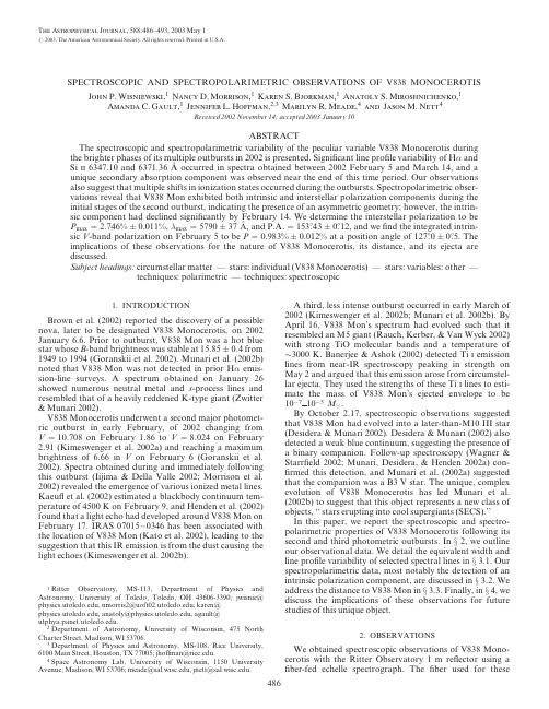
SPECTROSCOPIC AND SPECTROPOLARIMETRIC OBSERVATIONS OF V838MONOCEROTISJohn P.Wisniewski,1Nancy D.Morrison,1Karen S.Bjorkman,1Anatoly S.Miroshnichenko,1Amanda C.Gault,1Jennifer L.Hoffman,2,3Marilyn R.Meade,4and Jason t 4Received 2002November 14;accepted 2003January 10ABSTRACTThe spectroscopic and spectropolarimetric variability of the peculiar variable V838Monocerotis during the brighter phases of its multiple outbursts in 2002is presented.Significant line profile variability of H andSi ii 6347.10and 6371.36A˚occurred in spectra obtained between 2002February 5and March 14,and a unique secondary absorption component was observed near the end of this time period.Our observations also suggest that multiple shifts in ionization states occurred during the outbursts.Spectropolarimetric obser-vations reveal that V838Mon exhibited both intrinsic and interstellar polarization components during the initial stages of the second outburst,indicating the presence of an asymmetric geometry;however,the intrin-sic component had declined significantly by February 14.We determine the interstellar polarization to be P max ¼2:746%Æ0:011%, max ¼5790Æ37G ,and P :A :¼153=43Æ0=12,and we find the integrated intrin-sic V -band polarization on February 5to be P ¼0:983%Æ0:012%at a position angle of 127=0Æ0=5.The implications of these observations for the nature of V838Monocerotis,its distance,and its ejecta are discussed.Subject headings:circumstellar matter —stars:individual (V838Monocerotis)—stars:variables:other —techniques:polarimetric —techniques:spectroscopic1.INTRODUCTIONBrown et al.(2002)reported the discovery of a possible nova,later to be designated V838Monocerotis,on 2002January 6.6.Prior to outburst,V838Mon was a hot blue star whose B -band brightness was stable at 15:85Æ0:4from 1949to 1994(Goranskii et al.2002).Munari et al.(2002b)noted that V838Mon was not detected in prior H emis-sion-line surveys.A spectrum obtained on January 26showed numerous neutral metal and s -process lines and resembled that of a heavily reddened K-type giant (Zwitter &Munari 2002).V838Monocerotis underwent a second major photomet-ric outburst in early February,of 2002changing from V ¼10:708on February 1.86to V ¼8:024on February 2.91(Kimeswenger et al.2002a)and reaching a maximum brightness of 6.66in V on February 6(Goranskii et al.2002).Spectra obtained during and immediately following this outburst (Iijima &Della Valle 2002;Morrison et al.2002)revealed the emergence of various ionized metal lines.Kaeuflet al.(2002)estimated a blackbody continuum tem-perature of 4500K on February 9,and Henden et al.(2002)found that a light echo had developed around V838Mon on February 17.IRAS 07015À0346has been associated with the location of V838Mon (Kato et al.2002),leading to the suggestion that this IR emission is from the dust causing the light echoes (Kimeswenger et al.2002b).A third,less intense outburst occurred in early March of 2002(Kimeswenger et al.2002b;Munari et al.2002b).By April 16,V838Mon’s spectrum had evolved such that it resembled an M5giant (Rauch,Kerber,&Van Wyck 2002)with strong TiO molecular bands and a temperature of $3000K.Banerjee &Ashok (2002)detected Ti i emission lines from near-IR spectroscopy peaking in strength on May 2and argued that this emission arose from circumstel-lar ejecta.They used the strengths of these Ti i lines to esti-mate the mass of V838Mon’s ejected envelope to be 10À710À5M .By October 2.17,spectroscopic observations suggested that V838Mon had evolved into a later-than-M10III star (Desidera &Munari 2002).Desidera &Munari (2002)also detected a weak blue continuum,suggesting the presence of a binary companion.Follow-up spectroscopy (Wagner &Starrfield 2002;Munari,Desidera,&Henden 2002a)con-firmed this detection,and Munari et al.(2002a)suggested that the companion was a B3V star.The unique,complex evolution of V838Monocerotis has led Munari et al.(2002b)to suggest that this object represents a new class of objects,‘‘stars erupting into cool supergiants (SECS).’’In this paper,we report the spectroscopic and spectro-polarimetric properties of V838Monocerotis following its second and third photometric outbursts.In x 2,we outline our observational data.We detail the equivalent width and line profile variability of selected spectral lines in x 3.1.Our spectropolarimetric data,most notably the detection of an intrinsic polarization component,are discussed in x 3.2.We address the distance to V838Mon in x 3.3.Finally,in x 4,we discuss the implications of these observations for future studies of this unique object.2.OBSERVATIONSWe obtained spectroscopic observations of V838Mono-cerotis with the Ritter Observatory 1m reflector using a fiber-fed echelle spectrograph.The fiber used for these 1Ritter Observatory,MS-113,Department of Physics and Astronomy,University of Toledo,Toledo,OH 43606-3390;jwisnie@,nmorris2@,karen@,anatoly@,agault@.2Department of Astronomy,University of Wisconsin,475North Charter Street,Madison,WI 53706.3Department of Physics and Astronomy,MS-108,Rice University,6100Main Street,Houston,TX 77005;jhoffman@.4Space Astronomy Lab,University of Wisconsin,1150University Avenue,Madison,WI 53706;meade@,jnett@.The Astrophysical Journal ,588:486–493,2003May 1#2003.The American Astronomical Society.All rights reserved.Printed in U.S.A.486observations has a diameter of200l m,which corresponds to roughly500on the sky.Nine nonadjacent orders of a width of70A˚were observed in the range5285–6595A˚. Data were recorded on a1200Â800Wright Instruments D,with22:5Â22:5l m pixels.With R =D ’26;000;the spectral resolution element,D ,is about4.2pixels owing to a widened entrance slit.Observations were reduced with IRAF5using standard techniques.Fur-ther details about the reduction of Ritter data can be found in Morrison et al.(1997).Unless otherwise noted,all data were shifted to the heliocentric rest frame and continuum normalized.We obtained spectropolarimetric observations of V838 Mon with the University of Wisconsin’s Halfwave Polar-imeter(HPOL)spectropolarimeter,which is the dedicated instrument on the0.9m Pine BluffObservatory(PBO)tele-scope.These data were recorded with a400Â1200pixel CCD camera,covering the wavelength range of3200–10500 A˚,with a spectral resolution of7A˚below6000A˚and10A˚above this point(Nordsieck&Harris1996).Observations were made with dual600Â1200apertures,with the600slit aligned east-west and the1200decker aligned north-south on the sky.The two apertures allow simultaneous star and skydata to be recorded,providing a reliable means for subtrac-tion of background sky polarization and,hence,allowing accurate observations to be made even in nonphotometric skies.We processed these data using REDUCE,a spectro-polarimetric software package developed by the University of Wisconsin–Madison(Wolff,Nordsieck,&Nook1996). Further details about HPOL and REDUCE may be found in Nook(1990)and Harries,Babler,&Fox(2000).Instru-mental polarization is monitored on a weekly to monthly basis at PBO via observations of polarized and unpolarized standard stars,and over its13yr existence,HPOL has proved to be a very stable instrument.We have corrected our data for instrumental effects to an absolute accuracy of 0.025%and1 in the V band(K.H.Nordsieck,2002,private communication).HPOL spectroscopic data are not cali-brated to an absoluteflux level due to the nonphotometric skies routinely present(Harries et al.2000).Table1pro-vides a log of the observations from both observatories.3.RESULTS3.1.Spectroscopic VariabilityWe now discuss the spectral evolutionary history of V838 Monocerotis from February5to March14.Our observa-tions of V838Mon from February5to February9,during the onset of the second photometric outburst,indicate an overall shift toward a higher ionization state(Iijima&Della Valle2002;Morrison et al.2002)as compared with initial observations(Zwitter&Munari2002).H shows a strong P Cygni profile,with electron scatter-ing wings extending at leastÆ1100km sÀ1from February5 to February8and about850km sÀ1on February9,and an average heliocentric blue-edge radial velocity ofÀ300km sÀ1(see Fig.1and Table2).This radial velocity is slightly lower than the terminal velocity ofÀ500km sÀ1observed in late January in Ca ii,Ba ii,Na i,and Li i lines(Munari et al.2002c).Goranskii et al.(2002)report that a spectrum on February5shows H with FWZI=3100km sÀ1and an absorption component atÀ300km sÀ1,which is inconsis-tent with ourfindings.The extent of the electron scattering wings strongly depends on accurate continuum placement. We are confident that,within the limits of the signal-to-noise ratio of our data,we see a5A˚‘‘flat’’continuum region at each end of the spectral interval containing H ; hence,we are accurately determining the continuum level. The total equivalent width peaked on February6(see Table 3)and then began a steady decrease.Equivalent width errors were calculated using 2¼N½h =ðS=NÞ 2ðfÃ=f cÞ, where N is the number of pixels across a line,h is the disper-sion in A˚pixelÀ1,fÃis theflux in the line,f c is theflux at the continuum,and S/N is the signal-to-noise ratio(Chalabaev &Maillard1983).In early February,all the strong lines exhibited significant line profile variability.In H (Fig.1),the emission peak migrated to longer wavelengths with time.The high-velocity component of Si ii6347.1and6371.4A˚(Fig.2)weakens with time,and the intrinsic component of Na i5889.95and 5895.9A˚(Fig.3)also shows variability.Note that since the interstellar Na i components appear to be saturated,they could notfit with Gaussians and subtracted to reveal the pure intrinsic component.The low-resolution HPOL spec-trum(Fig.4)on February8clearly depicts the P Cygni pro-files of Fe ii4923.9,5018.4,and5169.0A˚and the Ca ii infrared triplet8498.0,8542.1,and8662.1A˚.Hydrogen Paschen absorption lines at8438.0,8467.3,8598.4,8750.5, 8862.8,9014.9,and9229.0A˚are observed,as well as H i 10049.4A˚,which has a clear P Cygni profile.By February14,the P Cygni profile of H had weakened considerably(Table3,Fig.1),and its absorption and emis-sion components were approaching equality in strength. The strong electron scattering wings previously observed had disappeared by our February14observation.Goran-skii et al.(2002)noted that the H electron scattering wings had disappeared in their spectrum taken on February16. These results are consistent with a decreasing excitation level in the circumstellar envelope.A low-resolution red5IRAF is distributed by the National Optical Astronomy Observatory, which is operated by the Association of Universities for Research in Astronomy,Inc.,under contract with the National Science Foundation.TABLE1Summary of ObservationsSignalÀtoÀNoise Ratios 2002D ate(UT)MJD O bservatory H Si ii Fe i Na i Feb5..........2,452,310.7Rit2422 (18)Feb6..........2,452,311.7Rit8468 (42)Feb8..........2,452,313.6Rit4842 (32)Feb8..........2,452,313.7HPOL............ Feb9..........2,452,314.7Rit6664 (46)Feb13........2,452,318.8HPOL............ Feb14........2,452,319.7Rit42 (28)Feb19........2,452,324.6Rit14......... Mar11.......2,452,344.6Rit6064 (32)Mar14.......2,452,347.6Rit104847834 Note.—‘‘Rit’’denotes Ritter spectroscopy and HPOL denotes HPOL spectropolarimetry.Multiple observations during one night were co-added using standard IRAF techniques to increase the signal-to-noise ratio.The modified Julian dates listed correspond to the midpoint of the observations for a specific night.The signal-to-noise ratios cited are the signal-to-noise ratios per resolution element,calculated in line-free regions of the spectrum.V838MONOCEROTIS487HPOL spectrum obtained on February 13(Fig.5)reveals two other qualitative changes:the emission components of both the P Cygni Ca ii infrared triplet lines and H i 10049.4A˚line significantly decreased in strength.By the end of the third photometric outburst,a significant shift in V838Mon’s spectral characteristics had occurred.Specifically,our spectra on March 11showed that a second high-velocity absorption component had developed in a few lines.H (Fig.1)clearly shows this component centered at a radial velocity of À200km s À1with a blue-edge radial velocity of À280km s À1.Figure 2shows that this feature isalso present in the Si ii 6347.1A˚line centered at À200km s À1with a blue-edge radial velocity of À260km s À1and inthe Si ii 6371.4A˚line centered at À140km s À1with ablue-Fig.1.—H line profiles sorted chronologically.From shorter to longer wavelengths,the tick marks denote À1000,À500,500,and 1000km s À1,respectively.TABLE 2Observed Spectral Lines and Their General CharacteristicsModified Julian DateLine 2,452,310.62,452,311.62,452,313.62,452,314.62,452,318.72,452,319.62,452,324.62,452,344.62,452,347.6H ............................e 1..................Fe ii 4923.9A ˚............p 1..................Fe ii 5018.4A ˚............p 1..................Fe ii 5169.0A ˚............p 1..................Fe ii 5316.2A ˚......p p p 1p ...p?...a a Na i 5889.95A ˚....p p p p ...p ...p p Na i 5895.9A ˚......p p p p ...p ...p p Fe i 6191.6A ˚............................p p Si ii 6347A ˚..........p p p p .........p 2p 2Si ii 6371A˚..........p p p p .........p 2p 2N ii 6380A˚..........a a a a .........a a Fe i 6393.6A˚............................p 2p 2H ......................p p p p p 1p p p 2p 2C ii 6576A˚...............................e e C ii 6583A˚...............................e e Ca ii 8498A ˚..............p 1...p 1............Ca ii 8542A ˚..............p 1...p 1............Ca ii 8662A˚..............p 1...p 1............Paschen.....................a 1...a 1............H i 10049.4A˚............p?1...p?1............Note.—Notation of p =P Cygni profile;a =absorption;e =emission.Superscript ‘‘1’’denotes line identification via low-resolution HPOL spectropolarimetry.Superscript ‘‘2’’denotes multiple absorption components observed.488WISNIEWSKI ET AL.Vol.588edge radial velocity ofÀ190km sÀ1.On the basis of the radial velocities of these dual absorption features,we iden-tify the enormous P Cygni profile around6394A˚seen in Figure2as Fe i6393.6A˚.A strong P Cygni–profiled line in the vicinity of6190A˚,which we attribute to Fe i6191.6A˚, also emerged on March11(Fig.6).Figure1also reveals new spectroscopic features at6544.9,6577.2,and6582.5A˚, which we attribute to Mg ii6545.9A˚and C ii6578.1and 6582.9A˚.The apparent emergence of both higher excitation lines(C ii and Mg ii)simultaneously with lower excitation lines(Fe i)illustrates the complexity of V838Mon’s out-burst.In fact,nearly all nine orders of our spectra show evi-dence for the emergence of new spectral features on March 11and14.Because of the low signal-to-noise ratios as well as uncertainties in line blending and profile shapes,we are unable to identify all lines definitively.Since many of these lines are consistent with the rest wavelengths of Fe i,Ne i, Ni i,Ti ii,Mg ii,and Fe ii,and since,as noted above,we have positively identified two lines of Fe i emerging on March11,these results indicate that V838Mon began to experience a shift to a lower ionization state.The evidence for spectral evolution that we observed will need to be com-bined with that of other authors to portray a comprehensive picture of V838Mon’s outbursts.3.2.Spectropolarimetric VariabilityFigures5and6illustrate the wavelength-dependent polarization of V838Mon on February8and13,respec-tively.The differences between these two observations are readily apparent.The integrated Johnson R-band polariza-tion of the February8data is P¼3:226%Æ0:004%at a position angle of149=0Æ0=1,while the R-band polariza-tion of the later observation is P¼2:667%Æ0:004%at a position angle of153=4Æ0=1.This change strongly suggests the presence of an intrinsic polarization component.TABLE3Equivalent Width in A˚of Selected Spectral Lines for the Eight Nights of Ritter ObservationsModified Julian DateL ine2,452,310.62,452,311.62,452,313.62,452,314.62,452,319.62,452,324.62,452,344.62,452,347.6H (total)...................À29.15Æ0.75À34.22Æ0.25À33.42Æ0.43À27.88Æ0.26À9.01Æ0.15À3.40Æ0.26À0.66Æ0.03À0.73Æ0.02 Si ii6347A˚(abs)........ 1.49Æ0.06 1.22Æ0.020.80Æ0.020.81Æ0.02......0.53Æ0.010.45Æ0.01 Si ii6347A˚(em).........À0.28Æ0.02À0.36Æ0.01À0.35Æ0.01À0.29Æ0.01......À0.11Æ0.01À0.12Æ0.01 Si ii6371A˚(abs)........0.90Æ0.050.81Æ0.020.48Æ0.020.45Æ0.01......0.43Æ0.010.37Æ0.01 Si ii6371A˚(em).........À0.31Æ0.02À0.30Æ0.01À0.25Æ0.01À0.25Æ0.01......À0.25Æ0.01À0.23Æ0.01 N ii6380A˚.................0.19Æ0.010.15Æ0.010.13Æ0.010.13Æ0.01......0.12Æ0.010.13Æ0.01 Fe ii5316.2A˚(abs)..... 1.98Æ0.16 1.51Æ0.07 1.65Æ0.10 1.42Æ0.06 1.03Æ0.09...0.77Æ0.080.55Æ0.04 Fe ii5316.2A˚(em).....À2.27Æ0.20À2.39Æ0.11À2.76Æ0.17À3.01Æ0.10À2.87Æ0.20...À0.55Æ0.09À0.63Æ0.06 Note.—Except for H ,all measurements were made on spectra smoothed with a boxcar function of size3.Fig.2.—Si ii6347.1and6371.4A˚line profiles sorted chronologicallyNo.1,2003V838MONOCEROTIS489Furthermore,the February 8data are characterized by strongly depolarized emission lines,while the February 13polarimetric data show no line features.Polarimetric studies of Be stars (Harrington &Collins 1968;Coyne 1976)have found that,in contrast to continuum photons,line emission,which originates predominantly in Be circumstellar disks,has a low probability of being scattered.With a few excep-tions (McLean &Clarke 1979;Quirrenbach et al.1997),emission lines should show little to no intrinsic polarization.Thus,an intrinsically polarized emission-line star should exhibit depolarized emission lines,e.g.,a superposition of polarized continuum flux and unpolarized line flux.If one employs a similar argument with the ejecta of V838Mon,the strongly depolarized emission lines of February 8may be used to infer the interstellar polarization component (ISP).Similarly,the absence of depolarization effects in the February 13data suggests that this polarization minima may be attributed primarily to interstellar polarization.As previously noted,the electron scattering wings of H disap-peared by February 14.Since one expects electron scattering in the ejecta of V838Mon to be the primary source of any intrinsic polarization,the disappearance of the electron scattering wings is consistent with the hypothesis that the polarization signal observed on February 13is primarily interstellar in nature.In order to parametrize the wavelength dependence of the interstellar polarization in the February 13data,we fitted the empirical Serkowski law (Serkowski,Mathewson,&Ford 1975),as modified by Wilking,Lebofsky,&Rieke (1982),to these data.The resulting ISP parameters are P max ¼2:746%Æ0:011%, max ¼5790Æ37G ,P :A :¼153=43Æ0=12, P :A :¼0,and K ¼0:971.This fit is overlaid in Figures 4and 5.The Serkowski fit provides a near-perfect fit to the February 13observation;furthermore,it fits nicely the depolarized emission lines in the February 8observa-tion.We qualitatively cross-check this claim by using the polarization and extinction relationship formulated by Serkowski et al.(1975),3E B ÀV P max 9E B ÀV .Munari et al.(2002c)established a lower limit for the interstellar red-dening of E B ÀV $0:25and suggested that the finding of Zwitter &Munari (2002),E B ÀV ¼0:80Æ0:05,represents an upper limit.Following the arguments of Munari et al.(2002c),we adopt the midpoint of these values,E B ÀV ¼0:50,which bounds the interstellar polarization along the line of sight to V838Mon by 1:5% P max 4:5%and,thus,qualitatively agrees with our ISP determination.Munari et al.(2002c)reported preliminary polarimetry results in which they suggested the ISP is characterized byP max ¼2:6%at 5500A˚at a position angle of 150 Æ2 .We are thus confident that our parametrization accurately describes the interstellar polarization component.We used these Serkowski parameters to remove the ISP component from the February 8data,as seen in Figure 4,leaving only the intrinsic component.We find the integrated V -band intrinsic polarization to be P ¼0:983%Æ0:012%at a position angle of 127=0Æ0=5.It is interesting that the intrinsic polarization clearly is not wavelength independent,which one would expect in the case of pure electron scatter-ing.Rather,the polarization gradually increases at wave-lengths shortward and longward of $8000A˚,which suggests the presence of an absorptive opacity source in V838Mon’s ejecta.A possible Paschen jump,albeit only at a 1 detection level,is visible in the raw and intrinsic polarization in Figure bined with the spectroscopic observations of strong H electron scattering wings on Feb-ruary 8,this might suggest that hydrogen is the opacity source (Wood et al.1996;Wood,Bjorkman,&Bjorkman1997).Fig.3.—Na i 5889.95and 5895.92A˚line profiles sorted chronologically.Note that the narrow interstellar line components are superposed on the intrinsic components.As discussed in x 3.1,the saturation of the interstellar components prevents the isolation of the intrinsic components.490WISNIEWSKI ET AL.Vol.5883.3.Distance EstimationsThe distance to V838Mon has yet to be agreed upon.Munari et al.(2002b,2002c)followed the propagation of V838Mon’s light echo,assuming a spherical distribution of scattering material,to derive a distance of 790Æ30pc.Kimeswenger et al.(2002b)used the same technique on a different data set to estimate a distance of 640–680pc.Bond et al.(2002)estimated a distance of 2.5kpc from Hubble Space Telescope light echo images;however,it has been sug-gested that the geometry assumed by these authors is unreal-istic (Munari et al.2002c;Kimeswenger et al.2002b).More recently,the reported detection of a hot binary companion (Desidera &Munari 2002;Wagner &Starrfield 2002;Munari et al.2002a)has led Munari et al.(2002a)to suggest a distance of 10–11kpc on the basis of spectrophotometric parallax.We add to the above discussion by considering the distance implied by our spectroscopic and polarimetric observations.On the basis of the assumption that cataclysmic variables contain no intrinsic polarization,Barrett (1996)suggested a rough relationship between polarization and distance.When applied to sources near the Galactic plane for distan-ces 1kpc,this relation is given by P =d ¼3:6%kpc À1.Given our estimate of P max of 2.746%,this would suggest a distance to V838Mon of 763pc.V838Mon’s strong,double interstellar Na i D lines pro-vide a different constraint on the distance.At Galactic longi-tude 217=8,radial velocities of objects outside the solar circle are positive and increase monotonically with increas-ing distance from the Sun.Thus,the radial velocity of the longer wavelength component provides a lower limit on the distance to V838Mon.The radial velocities of the two com-ponents of the D lines were measured in the spectra of February 5,6,8,and 9.For D1and D2,the means and stan-dard deviations were,respectively,21:9Æ0:6,22:1Æ0:8,47:9Æ0:8,and 47:5Æ2:8km s À1relative to the LSR.Note that our data are accurate to 2km s À1as compared to the IAU velocity standard Gem,which is constant to better than 0.1km s À1(Larson et al.1993).To read offthe distance of the 48km s À1,more distant cloud,we used the velocity contour map by Brand &Blitz (1993),which does not assume the velocity field of Galactic rotation to be axisymmetric.The Galactic longitude of V838Mon coincides with an interesting feature in this map,an ‘‘island ’’of high velocities of about 50km s À1located about 2500pc from the Sun.We estimate that distances con-sistent with this velocity map,for a radial velocity of+48Fig.4.—HPOL spectropolarimetry from February 8.Upper panel :Flux in units of ergs cm À2s À1A ˚À1,with the red data magnified by a factor of 2.Second and third panels from top :Total polarization and position angle where the red data,e.g.,6000–10500A ˚,are binned to a constant error of 0.075%and blue data,e.g.,3200–6000A˚,are binned to a constant error of 0.12%.Overplotted is the derived Serkowski interstellar polarization component,whose parameters are given by P max ¼2:746%Æ0:011%, max ¼5790Æ37G ,P :A :¼153=43Æ0=12, P :A :¼0,and K ¼0:971.Lower two panels :Intrinsic polarization and posi-tion angle binned to constant errors of 0.07%and 0.10%for the red and blue data,respectively.The wavelength dependence of the intrinsic polarization is not representative of pure electron scattering;rather,it implies the presence of an opacity source such as hydrogen.No.1,2003V838MONOCEROTIS 491Fig.5.—HPOL spectropolarimetry from February13.Upper panel:Flux in units of ergs cmÀ2sÀ1A˚À1.Middle and lower panels:Total polarization and position angle binned to a constant error of0.074%.Solid line:Fitted interstellar polarization component.The intrinsic polarization that was present on February8clearly has disappeared by February13.Fig.6.—A strong P Cygni profile,attributed to Fe i6191.6A˚,is shown in a noncontinuum normalized spectrum from March14km sÀ1,lie in the range2500Æ300pc.This estimate consti-tutes our lower limit on the distance to V838Mon.Veloc-ities as large as50km sÀ1are not reached again in this direction at heliocentric distances less than8kpc.Since this lower limit is greater than1kpc,the distance estimation technique used with our polarimetric data is no longer applicable.4.DISCUSSIONOur spectroscopic data offer both qualitative and quanti-tative insight into the initial stages of the2002outburst. Future modeling efforts can be constrained by the equiva-lent width variability of the lines presented.Furthermore, the complex line profile variability and evolution of various species and ionization stages of lines presented in this paper should also provide constraints on future attempts to explain this outburst.In spite of our sparse polarimetric data,these observa-tions clearly demonstrate that the ejecta of V838Monocero-tis deviated significantly from a spherical geometry.We note the similarity between our observations and those of Bjorkman et al.(1994),who found Nova Cygni1992to have an intrinsic polarization signal during the initial stages of outburst.These authors suggest the intrinsic polarization during this initial stage was caused by electron scattering in a slightlyflattened spheroidal shell.As the shell expanded, the electron scattering optical depth decreased;hence,the intrinsic polarization declined.A similar interpretation could be applied to V838Mon.The electron scattering wings around H were sizable on February5but clearly had weakened by February9and disappeared by February 14.Coupled with our discovery of an intrinsic polarization component present on February8but gone by February13, this picture of an expanding,flattened spheroidal shell could provide a viable explanation of the intrinsic polarization observed during the2002outburst.Finally,we consider the implications of these observa-tions for future studies of this object.Munari et al.(2002c) and Kimeswenger et al.(2002b)discuss different classifica-tions of V838Mon,including a nova outburst,a post-AGB star,an M31red–type variable,and a V4332Sgr–type varia-ble:both suggest that V838Mon is most similar to a V4332 Sgr–type variable.As described above,we suggest that the geometry of the outburst,as probed by polarimetry,might be similar to that of a nova outburst.This suggests that the geometry of V4332Sgr’s,V838Mon’s,and nova outbursts might be similar.It would be worthwhile to measure the polarization of V4332Sgr today to verify that,like V838 Mon,it has no intrinsic polarization at a time long after out-burst.Furthermore,we suggest that polarimetric observa-tions immediately following the outbursts of all future V4332Sgr–type variables be made.Such observations would provide an ideal test bed to correlate the geometry of each outburst and,hence,help to identify the true nature of these unique objects.We would like to thank Kenneth H.Nordsieck for pro-viding access to the HPOL spectropolarimeter.We also thank Brian Babler for his help with various aspects of HPOL data reduction and management.We thank the anonymous referee for helping to improve this paper.Sup-port for observational research at Ritter Observatory has been provided by the University of Toledo,with technical support provided by R.J.Burmeister.K.S.B.is a Cottrell Scholar of the Research Corporation and gratefully acknowledges their support.This research has made use of the SIMBAD database operated at CDS,Strasbourg, France,and the NASA ADS system.REFERENCESBanerjee,D.P.K.,&Ashok,N.M.2002,A&A,395,161Barrett,P.1996,PASP,108,412Bjorkman,K.S.,Johansen,K.A.,Nordsieck,K.H.,Gallagher,J.S.,& Barger,A.J.1994,ApJ,425,247Bond,H.E.,Panagia,N.,Sparks,W.B.,Starrfield,S.G.,Wagner,R.M., &Henden,A.A.2002,IAU Circ.7943Brand,J.,&Blitz,L.1993,A&A,275,67Brown,N.J.,et al.2002,IAU Circ.7785Chalabaev,A.,&Maillard,J.P.1983,A&A,127,279Coyne,G.V.1976,A&A,49,89Desidera,S.,&Munari,U.2002,IAU Circ.7982Goranskii,V.P.,Kusakin,A.V.,Metlova,N.V.,Shugarov,S.Y., Barsukova,E.A.,&Borisov,N.V.2002,Astron.Lett.,28,691 Harries,T.J.,Babler,B.L.,&Fox,G.K.2000,A&A,361,273 Harrington,J.P.,&Collins,G.W.,II.1968,ApJ,151,1051Henden,A.,Munari,U.,&Schwartz,M.2002,IAU Circ.7859Iijima,T.,&Della Valle,M.2002,IAU Circ.7822Kaeufl,J.U.,Locurto,G.,Kerber,F.,&Heijligers,B.2002,IAU Circ. 7831Kato,T.,Yamaoka,H.,&Kiyota,S.2002,IAU Circ.7786 Kimeswenger,S.,Lederle,C.,&Schmeja,S.2002a,IAU Circ.7816 Kimeswenger,S.,Lederle,C.,Schmeja,S.,&Armsdorfer, B.2002b, MNRAS,336,L43Larson,A.M.,Irwin,A.W.,Yang,S.L.S.,Goodenough,C.,Walker, G.A.H.,Walker,A.R.,&Bohlender,D.A.1993,PASP,105,825McLean,I.S.,&Clarke,D.1979,MNRAS,186,245Morrison,N.D.,Bjorkman,K.S.,Miroshnichenko,A.,&Wisniewski, J.P.2002,IAU Circ.7829Morrison,N.D.,Knauth,D.C.,Mulliss,C.L.,&Lee,W.1997,PASP, 109,676Munari,U.,Desidera,S.,&Henden,A.2002a,IAU Circ.8005Munari,U.,Henden,A.,Corradi,R.L.M.,&Zwitter,T.2002b,in AIP Conf.Proc.63,Classical Nova Explosions,ed.M.Hernanz&J.Jose (New York:AIP),52Munari,U.,et al.2002c,A&A,389,L51Nook,M.1990,Ph.D.dissertation,Univ.Wisconsin–Madison Nordsieck,K.H.,&Harris,W.1996,in ASP Conf.Ser.97,Polarimetry of the Interstellar Medium,ed.W.G.Roberge&D.C.B.Whittet (San Francisco:ASP),100Quirrenbach,A.,et al.1997,ApJ,479,477Rauch,T.,Kerber,F.,&Van Wyk,F.2002,IAU Circ.7886 Serkowski,K.,Mathewson,D.S.,&Ford,V.L.1975,ApJ,196,261 Wagner,R.M.,&Starrfield,S.G.2002,IAU Circ.7992Wilking,B.A.,Lebofsky,M.J.,&Rieke,G.H.1982,AJ,87,695Wolff,M.J.,Nordsieck,K.H.,&Nook,M.A.1996,AJ,111,856 Wood,K.,Bjorkman,K.S.,&Bjorkman,J.E.1997,ApJ,477,926 Wood,K.,Bjorkman,J.E.,Whitney,B.,&Code,A.1996,ApJ,461,847 Zwitter,T.,&Munari,U.2002,IAU Circ.7812V838MONOCEROTIS493。

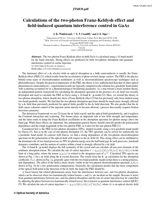
Calculations of the two-photon Franz-Keldysh effect andfield-induced quantum interference control in GaAsJ.K.Wahlstrand,1,2S.T.Cundiff,2and J.E.Sipe2,∗1Department of Physics,University of Maryland,College Park,Maryland20742,USA2JILA,University of Colorado and National Institute of Standards and Technology,Boulder,Colorado80309-0440,USA∗Permanent address:Department of Physics,University of Toronto,Toronto,Ontario M5S1A7,Canadaemail:wahlstrj@Abstract:The two-photon Franz-Keldysh effect in bulk GaAs is calculated using a14-band modelfor the band structure.Strong effects are predicted for both two-photon absorption and quantuminterference control of carrier injection.c 2010Optical Society of AmericaOCIS codes:(190.4180)Multiphoton processesThe dominant effect of a dc electricfield on optical absorption in a bulk semiconductor is usually the Franz-Keldysh effect(FKE)[1],which results from the acceleration of photo-excited charge carriers.The FKE is the physics behind some types of electroabsorption modulators as well as electromodulation spectroscopy techniques such as photoreflectance.Despite the practical importance of the FKE,the theory is less sophisticated than that of other optical phenomena in semiconductors–experimental results are typically compared to the solution for a parabolic band model, with scattering accounted for in a phenomenological broadening parameter.As a step toward a more modern theory, an independent-particle framework for calculating the absorption spectrum in the presence of a dcfield was recently developed and used to calculate the FKE in GaAs using a14-band k·p model[2].Here,we extend this theory to two-photon absorption,which should also show a Franz-Keldysh effect[3]but has previously only been studied using two-band parabolic models.Wefind that the two-photon absorption spectrum should be much more strongly affected by a dcfield than previously predicted for opticalfields parallel to the dcfield direction.We also predict that the dc field causes coherent control of the injected carrier density to become allowed,a process that usually requires broken inversion symmetry.The theoretical framework we use[2]treats the dcfield exactly and the opticalfield perturbatively,and it neglects the Coulomb interaction and scattering.The former plays an important role at lowfield strength and temperature, and the latter tends to damp the Franz-Keldysh oscillations in the absorption spectrum for photon energy above the band gap.While these effects are important,this independent-particle theory should correctly predict the polarization dependence and the rough magnitude of the two-photon FKE,as it does for the one-photon FKE[1].Consideredfirst is the FKE in two-photon absorption(TPA),studied recently using a two-parabolic-band model by Garcia[3].Just as in the case of one-photon absorption[1],the TPA spectrum can be solved for analytically fora parabolic band model.In contrast with Garcia,wefind a strong dependence of the two-photon electroabsorptionspectrum on the polarization of the opticalfield with respect to the dcfield[4].This strong effect can be attributed to the dominant role of two-band processes in TPA for photon energy near the half band gap.In such processes,intraband dynamics contribute,and the motion of carriers within a band is strongly affected by a dcfield.The14-band k·p model displays the full symmetry of the crystal and can calculate all non-zero elements of the nonlinear absorption tensor.We calculate the rate of carrier injection˙n=ηijkl(ω)[E i(ω)E j(ω)]∗E k(ω)E l(ω)in the limit of a long pulse,where the tensorηijkl(ω)is related to the imaginary part ofχ(3).Calculated TPA spectra are shown in Fig.1for a dcfield along theˆz crystal direction.The results from the k·p calculation for the absorption coefficientβ(ω),shown in Fig.1a,generally agree with the two-band parabolic model in that there is a strong polariza-tion dependence.The effect of thefield is more clearly visible in the two-photon electroabsorption spectrum∆β(ω), shown in Fig.1b for a few polarization configurations.Generally,the calculations predict that the more components of the opticalfield point in the direction of the dcfield,the larger the FKE should be.A lesser known but related phenomenon arises from the interference between one-and two-photon absorption,which can be observed when two harmonically related beamsωand2ωare incident on the sample.Because it arises from quantum interference between one-and two-photon absorption and the rate of carrier injection may be controlled by adjusting the phase between two harmonically related waves,this is known as quantum interference control(QUIC)[5].We calculate the rate of carrier injection˙n=ηijk(ω)[E i(ω)E j(ω)]∗E k(2ω),where E l is an optical electricfield © Optical Society of Americaa0.750.800.850.900.95051015 b 0.750.800.850.900.951.5 1.00.50.00.51.0¯h ω(eV)¯h ω(eV)β(ω)(c m /G W )∆β(ω)(c m /G W )Fig.1.Calculated TPA spectra,showing the TPA coefficient β(ω)for light polarized along various crystal directions for a67kV/cm dc field along the z direction.(a)The TPA spectrum in the absence of a field (black),with the optical field linearlypolarized along the ˆxdirection (red)and the ˆz direction (blue).(b)Two-photon electroabsorption spectrum (the change in the absorption spectrum due to the field).Components shown are ηzzzz (ω)(blue),ηxxxx (ω)(red),ηxxzz (ω)(green),and ηxxyy (ω)(black).a0.700.750.800.850.900.95 1.00 20020406080 b 0.700.750.800.850.900.95 1.00020406080100120¯h ω(eV)¯h ω(eV)I m χ(2)(p m /V )I m χ(2)(p m /V )Fig.2.Calculated QUIC spectra,showing the magnitude of Im χ(2)ijk (ω)∝ηijk (ω)for light polarized along various crystaldirections for a 67kV/cm dc field along the ˆzdirection.(a)Field-induced QUIC spectra,in which there is no QUIC carrier injection in the absence of a dc fiponents shown are ηzzz (ω)(black),ηxxz (ω)(red),and ηxzx (ω)(blue).(b)Theconventional population control [5]element ηxyz (ω)with (black)and without (red)a dc field along the z direction.component.When no dc field is present,control of the carrier injection rate is only possible in a crystal lacking inversion symmetry [5].The field-free QUIC tensor for carrier injection is proportional to the imaginary part of the nonlinear susceptibility χ(2),so in GaAs the only nonzero component is ηxyz .We find that a dc electric field enables control for other tensor components as well [6].Figure 2shows QUIC spectra calculated using a 14-band model as a function of ¯h ωnear half the band gap (0.76eV)in GaAs.The field-induced QUIC spectrum,the subject of a recent experiment [6],is shown in Fig.2a for afew different polarization configurations.We find that a dc field enables QUIC especially for energies near the half band gap.The component ηxyz that is nonzero in the absence of a dc field,shown in Fig.2b,is affected by the dc field much as the one-and two-photon absorption spectra are,with an exponential tail for photon energy below and Franz-Keldysh oscillations above the half band gap.The calculations we have done so far neglect decoherence and scattering as well as Coulomb effects,but they should be accurate for experiments performed at low temperature with large applied dc fields.The prediction of a strong polarization dependence in two-photon absorption,in disagreement with previous theories,should stimulate interest in experiments.[1] D.E.Aspnes,“Electric-field effects on optical absorption near thresholds in solids,”Phys.Rev.147,554(1966).[2]J.K.Wahlstrand and J.E.Sipe,“Independent-particle theory of the Franz-Keldysh effect including interband coupling:Application to calculationof electroabsorption in GaAs,”Phys.Rev.B 82,075206(2010).[3]H.Garcia,“Tunneling assisted two-photon absorption:The nonlinear Franz-Keldysh effect,”Phys.Rev.B 74,035212(2006).[4]J.K.Wahlstrand,S.T.Cundiff,and J.E.Sipe,“Polarization dependence of the two-photon Franz-Keldysh effect,”arXiv:1010.3920(unpublished).[5]J.M.Fraser,A.I.Shkrebtii,J.E.Sipe,and H.M.van Driel,“Quantum interference in electron-hole generation in noncentrosymmetric semicon-ductors,”Phys.Rev.Lett.83,4192(1999).[6]J.K.Wahlstrand,H.Zhang,S.Kannan,D.S.Dessau,J.E.Sipe,and S.T.Cundiff,“Electric field-induced quantum interference control in asemiconductor:A new manifestation of the Franz-Keldysh effect,”arXiv:1008.1893(unpublished).。

Single-and double-helix chiralfiber sensorsVictor I.Kopp,1,*Victor M.Churikov,1Guoyin Zhang,1Jonathan Singer,1Christopher W.Draper,1Norman Chao,1Daniel Neugroschl,1and Azriel Z.Genack1,21Chiral Photonics,Inc.,Clifton,New Jersey07012,USA2Department of Physics,Queens College of the City University of New York,Flushing,New York11367,USA*Corresponding author:vickopp@Received March16,2007;revised May22,2007;accepted May23,2007;posted June15,2007(Doc.ID81153);published August8,2007Copropagating core and cladding modes in opticalfibers can be coupled by a grating with a period greatlyexceeding the wavelength,since their propagation constants are similar.In contrast to conventional long-period gratings,in which the modulation is imposed by exposing a photosensitive core to ultraviolet light,wehave created chiral long-period gratings with single-or double-helix symmetry by twisting opticalfibers withnonconcentric or noncircular cores,respectively,as they pass through a short heat zone.The difference in sym-metry between single-and double-helix gratings is manifested in their polarization properties.The use of thesegratings as sensors of liquid level and temperature is demonstrated.©2007Optical Society of AmericaOCIS codes:060.0060,060.2310,060.2340.1.INTRODUCTIONOpticalfibers can be designed so that transmission through thefiber core varies with such changing environ-mental factors as pressure,temperature,and the refrac-tive index of the surrounding medium[1,2].Optical trans-mission may change as a result of either broadband attenuation or a shift of narrow spectral features.Narrow peaks or dips in thefiber transmission or reflection spec-trum are produced by resonant optical interactions with periodicfibers.The use offiber gratings with narrow spec-tral features is advantageous,since the sensitivity to change is enhanced and a singlefiber line may be used to carry signals from a number of remote sensors with fea-tures at different wavelengths arrayed in series.Narrow spectral features are most commonly produced by creat-ing a periodic modulation of the effective refractive index along thefiber by exposing photosensitivefiber to a peri-odic pattern of ultraviolet radiation.Infiber Bragg grat-ings(FBGs),thefiber structure is modulated at a period as short as half the optical wavelength.FBGs reflect light within thefiber core over a range of wavelengths propor-tional to the index contrast along thefiber.The central wavelength of the reflection band is sensitive to the effec-tive refractive index of the core mode,which varies with temperature,and to the structure’s period,which depends upon both thefiber tension and temperature.When the fiber period greatly exceeds the optical wavelength,core and cladding modes are coupled when the difference in their propagation constants equals a multiple of the grat-ing constant.This leads to a series of narrow dips in the transmission spectrum.In this case,in addition to sensi-tivity to temperature and elongation,the spectral position of the dip is also sensitive to the refractive index of the surrounding medium,since this affects the propagation constant the of cladding modes.Thefiber refractive index is most often modulated by exposingfiber with a photosensitive germanium-doped core to modulated ultraviolet light[1].The ultraviolet ra-diation is modulated by the interference of two laser beams or of two orders of diffraction from a phase mask. Long gratings are produced by precisely overlapping suc-cessive interference patterns to produce an extended co-herent pattern of index variation.In gratings with peri-ods greatly exceeding the wavelength,the refractive index may also be modulated by microbending[3],such as may be produced by squeezing thefiber between corru-gated plates,or by local heating with a CO2laser[4]or an electric arc[5].Recently,long-period helicalfiber gratings exhibiting dips in the transmission spectrum have been produced by twisting uniformly heated standard single modefiber in which some nonconcentricity existed[6].A periodic helical structure may also be created via glass microforming as afiber preform passes through a miniature oven[7].In this process,thefiber preform may be similar to conventionalfiber with a diameter as thin as 100␮m.This fabrication approach produces a stable structure with double-or single-helix symmetry in bire-fringentfiber preforms or nonconcentricfibers,respec-tively.While double helix structures are polarization sen-sitive,single helix structures are polarization insensitive. Chiralfibers may be produced with lengths as short as a few hundred micronmeters or as long as several centime-ters.High contrast chiral gratings can be implemented in a broad range of glass materials,which need not be pho-tosensitive.In addition to gratings with constant pitch, gratings with engineered pitch profile and with abrupt changes in twist can be fabricated.Thesefibers can be used as sensors,polarizers,and lasers.Double-helix structures are created by twisting bire-fringentfiber preforms with concentric cores with 180degree rotation symmetry.The period then equals one half the turn so that the pitch is twice the period,P =2a.When the wavelength inside the structure,␭,is close to twice the period,␭ϳ2a=P,the propagation of core modes is directly analogous to propagation in liquid crys-tals.In these self-organized structures,the direction of0740-3224/07/100A48-5/$15.00©2007Optical Society of Americaaverage molecular orientation in the plane rotates with displacement perpendicular to the plane [8].This double-helix structure is also found in structured thin films com-posed of closely packed twisted columns with subwave-length diameter and spacing produced by oblique deposition on a rotating substrate [9].The sinusoidal modulation of these planar birefringent structures results in a single bandgap with modes at the band edge for co-handed light with the same sense of circular polarization as the handedness of the helical structure [10].Orthogo-nally polarized light is freely transmitted at all wave-lengths.In addition to coupling of counterpropagating core modes when P ϳ␭,light may be scattered out of the core into the fiber cladding when P Ͼ␭.In chiral long-period gratings (CLPGs),in which P ӷ␭,core and clad-ding modes are coupled.In traditional LPGs,core and cladding modes are coupled by the grating,when ␤core −␤clad =m ␤gr ,where ␤core and ␤clad are the propagation constants of the core and cladding,respectively,␤gr =2␲/a is the grating constant,and m is the diffraction or-der.A comparison of the wavelengths of the dips and cal-culated propagation constants in the double-helix CLPG shows that the dip corresponding to m =1is not observed.In short-period chiral gratings,in which the core mode is reflected within the core,the deficit in linear momen-tum is taken up by the grating as described in the phase-matching condition above.In this case,the angular mo-mentum of photons changes by two units of ប,since the sense of circular polarization of the counterpropagatingincident and scattered waves is the same.We expect that,analogously,the CLPG couples the cohanded core mode and the crosshanded cladding modes,since these differ in angular momentum by two units of ប.In chiral gratings with pitch intermediate between the short and long peri-ods,the wave is scattered out of the fiber.Except for the middle portion of this intermediate scattering band,scat-tering is polarization selective.This serves as the basis of linear and circular polarizers with bandwidths of over 100nm.In single-helix structures produced by twisting the fi-bers’nonconcentric cores,the period of the refractive in-dex is equal to the pitch,P =a .The periodic modulation of the propagation direction within the helical core does not have a planar analog,but it is similar to fiber long-period gratings produced by microbending.Because fibers al-ways possess some nonconcentricity,twisting optical fi-bers produces structures with a single-helix component of symmetry with period equal to the helical pitch.In prac-tice,we find that when the core is displaced less than 10%of the core diameter,chiral fibers with substantial bire-fringence function as double-helix structures.At present,there is no theory describing the polarization-selective op-tical interaction with twisted fibers,but the qualitative behavior is consistent with the description of scattering presented in [11].In this article,we compare the performance of CLPGs with double-and single-helix structure.We find that core modes are coupled to cladding modes via higher-order scattering in double-helix structures and via first-order scattering in single-helix structures.Whereas the double-helix CLPG is polarization sensitive,opticalpropagationFig.1.Side image and schematic of face image of the (a)double and (b)single-helix gratings studied.Note the offset of the core center in (b)from the fibercenter.Fig.2.(Color online)Ratio of right-to-left circularly polarized transmission through a double-helix CLPG.The inset shows the shift in the spectrum when the fiber is immersed ingasoline.Fig. 3.(Color online)Polarization-insensitive transmission through a single-helix CLPG.in single-helix structures is largely independent of polar-ization.The performance of single-and double-helix long-period gratings as level sensors are compared.Finally,the use of the single-helix long-period grating as a tempera-ture sensor is demonstrated.2.GRATING PREPARATION AND CHARACTERIZATIONImages of the double-and single-helix gratings studied are shown in Fig.1.The fiber preforms used were held be-tween a twisting motor affixed to the upper and lower translation stages.A right-or left-handed structure is produced depending on the sense of rotation of the twist-ing motor.The double-helix CLPGs were created using low-temperature glasses that are passed through a short heat zone of length of ϳ300␮m at a temperature above the softening point.The heating element is an Omega-shaped resistive wire.The high-index rectangular core has an aspect ratio of 1:2,as can be seen in the cross sec-tion shown in Fig.1(a).The refractive indices of the core and cladding are 1.7and 1.5,respectively.The corre-sponding birefringence of the fiber of 0.03is larger than the corresponding values of the index modulation that have been realized in photosensitive glasses.The ratio of co-to crosshanded transmission through a 55mm long CLPG with a pitch of 78␮m is shown in Fig.2.The inset shows the shift of a dip when the CLPG is dipped into gasoline.Single-helix chiral gratings were produced in silica glass fibers using the same apparatus used to produce double-helix fibers,except that the heat source was a power-stabilized focused CO 2laser.The custom fiber pre-form consists of an eccentric elliptical core with a cladding diameter of 140␮m.An example of a twisted fiber pro-duced from that preform is shown in Fig.1(b).The pre-form core has an elliptical shape with major and minoraxes of 6and 3␮m,respectively,with a core center dis-placed by approximately 2␮m from the center of the fiber.The indices of the core and cladding are 1.48and 1.45,re-spectively.Because the core is elliptical,the symmetry of the twisted fiber also has a double-helix component.How-ever,the light does not interact with a double-helix struc-ture in the first order of diffraction,and the optical prop-erties of the structure near the wavelength corresponding to first order diffraction are determined by the single-helix symmetry.The untwisted fiber is twisted to a con-stant pitch,and subsequently the twist is stopped.The twist acceleration and deceleration occur in less than two turns.The region of constant pitch is typically 17mm long.The transmission spectrum of the single helix CLPG shown in Fig.3is essentially polarization insensitive.Note that linearly polarized light is not maintained in the twisted birefringent fiber so that light may have arbitrary polarization at the output for linearly polarized incident light.The polarization insensitivity of single-helix CLPGs refers to the independence of transmission upon incident polarization when there is no polarization analyzer.3.LIQUID LEVEL SENSINGPotential applications of CLPGs to liquid level sensing are suggested by the results presented in Figs.4and 5for double-and single-helix gratings,respectively.The light transmission at the wavelength located at the edge of the transition dip is affected by the liquid level,as it is in con-ventional fiber LPGs [12].As in conventional LPGs,the transmission spectrum in CLPGs is shifted when the fiber is completely covered with liquid.However,the behavior of conventional and chiral gratings is quite different when the fiber is partially covered.In LPGs,dips in transmis-sion are observed peaked at the two wavelengths that cor-respond to the fiber’s being in or out of the liquid [12].Fig.4.(Color online)Transmission through a double-helix LPG at 1484.55nm versus gasolinelevel.Fig.5.(Color online)Transmission through a single-helix LPG at 1656nm versus alcohollevel.Fig.6.(Color online)Spectra of transmission dips of single-helix CLPG covered with alcohol at different heights.The dip with constant width shifts continuously with changingimmersion.Fig.7.(Color online)Wavelength of transmission dip of single-helix CLPG versus temperature.The temperature was measured with a thermocouple.This might be expected if the wave interacts separately with the two portions of the fiber grating.In contrast,in CLPGs,the dip shifts continuously as the level changes,without a change in linewidth.This is seen in the trans-mission spectra for the single-helix CLPG shown in Fig.6.This may indicate a coherent interaction with the entire length of the chiral fiber.The same manufacturing process of twisting glass fiber was used for single-and double-helix grating.The use of microforming as opposed to optical lithography enhances the long-term stability of the gratings in harsh environ-ment.Gasoline and alcohol were the liquids sensed,since fuel level sensors are an important potential application.4.TEMPERATURE SENSINGAs mentioned earlier,the single-helix grating was made from high-temperature silica fiber.This fiber is therefore a candidate as a high-temperature sensor.The tempera-ture testing was carried out in a computer-controlled high-temperature oven in which the temperature was monitored by a thermocouple.Both long-term tempera-ture stability and temperature sensitivity were tested us-ing a Micron Optics fiber interrogator in the temperaturerange 400–1100°e of the interrogator reduces the characterization and testing time and increases the accu-racy with which the dip position can be measured.In ad-dition,the dip position can be traced in real time.A mi-cromirror was attached to each CLPG so that it could be characterized in reflection,as required by the interroga-tor.The wavelength of the CLPG dip produced by the cou-pling of the core mode to the fourth cladding mode in a single-helix CLPG versus temperature is shown in Fig.7.We find that after annealing the dip wavelength shifts to the red by approximately 50nm,as the temperature is raised by 500°C.The sensitivity near 400°C is 0.11nm/°C,as seen in Fig.8.The shift is stable at a given temperature even after repeated cycling,as shown in Fig.8.The variation of the dip wavelength shown in Fig.8is characteristic of fluctuations over a few tempera-ture sweeps and does not reflect long-term drift.5.CONCLUSIONIn conclusion,the characteristics of single-and double-helix chiral fiber gratings that affect their performance as sensors is presented.The main differences and similari-ties of these gratings are summarized in Table 1.Chiral fiber gratings can be used in sensing heads for a wide range of sensing applications.Chiral fibers are particu-larly promising because they can continuously measure liquid levels,function in harsh environments,and be fab-ricated using a flexible procedure that does not require photosensitive glass and in an apparatus that can pro-duce many types of chiral devices.ACKNOWLEDGMENTSWe thank Alexander Tuder for help in preparing and characterizing twisted fibers.This work was supported by the U.S.Department of Commerce,National Institute of Standards and Technology,Advanced Technology Pro-gram,Cooperative Agreement Number 70NANB3H3038,and the National Science Foundation under grant DMR-0538350.REFERENCES1. A.Othonos and K.Kalli,Fiber Bragg Gratings:Fundamentals and Applications in Telecommunications and Sensing (Artech House,1999).2.S.W.James and R.P .Tatam,“Optical fibre long-period grating sensors:characteristics and application,”Meas.Sci.Technol.14,R49–R61(2003).3.C. B.Probst, A.Bjarklev,and S. B.Andreasen,“Experimental verification of microbending theory using mode coupling to discrete cladding modes,”J.Lightwave Technol.7,55–61(1989).4.D.D.Davis,T.K.Gaylord,E.N.Glytsis,S.G.Kosinski,S.C.Mettler,and A.M.Vengsarkar,“Long-period fibre grating fabrication with focused CO 2laser pulses,”Electron.Lett.34,302–303(1998).5.G.Rego,O.Okhotnikov,E.Dianov,and V .Sulimov,“High-temperature stability of long-period fiber gratings produced using an electric arc,”J.Lightwave Technol.19,1574–1579(2001).6.O.V .Ivanov,“Fabrication of long-period fiber gratings by twisting a standard single-mode fiber,”Opt.Lett.30,3290–3292(2005).7.V .I.Kopp,V .M.Churikov,J.Singer,N.Chao, D.Table 1.Key Parameters of Single andDouble-Helix CLPGsParameter Single Helix Double Helix Polarization insensitivity Yes No Independent use of orthogonal polarizations for multiplexing NoYesFabricated in low NA fibersYes NoEasily coupledto standard fiber Yes No Ultranarrow transmission dipsNoYesTemperature,strain,andtwist sensitivityYesYes Fig.8.(Color online)Wavelength of transmission dip of single-helix CLPG versus temperature.The temperature was continu-ously cycled around 400°C for 24h after the fiber was annealed for 2h at 800°C.Neugroschl,and A.Z.Genack,“Chiralfiber gratings,”Science305,74–75(2004).8.S.Chandrasekhar,Liquid Crystals(Cambridge U.Press,1977,1994).9.K.Robbie,D.J.Broer,and M.J.Brett,“Chiral nematicorder in liquid crystals imposed by an engineered inorganic nanostructure,”Nature(London)399,764–766(1999). 10.V.I.Kopp,B.Fan,H.K.M.Vithana,and A.Z.Genack,“Low-threshold lasing at the edge of a photonic stop bandin cholesteric liquid crystals,”Opt.Lett.23,1707–1709 (1998).11.V.I.Kopp,A.Z.Genack,V.M.Churikov,J.Singer,and N.Chao,“Chiralfiber gratings polarize light,”Photonics Spectra38,78(2004).12.S.Khaliq,S.W.James,and R.P.Tatam,“Fiber-opticliquid-level sensor using a long-period grating,”Opt.Lett.26,1224–1226(2001).。

Multimode Detection Performing FluorescencePolarization Assays on theVICTOR NivoIntroductionFluorescence Polarization (FP) is a homogeneous assay formatthat is highly suitable for many applications from occasionalusage to high throughput screening, due to rather inexpensive reagents and its signal stability1. In FP assays, polarized light isused to determine the rotation capabilities of smallfluorescently labelled molecules. With this assay principle, onecan indirectly detect whether tracer molecules are bound to amuch larger molecule or are freely rotating in solution. Theseare rather complex interrelationships on the assay as well as on the device side compared to other homogeneous, plate reader compatible assays. Hence, for users, it is often difficult to set up an FP assay correctly.For this reason, we describe in this T echnical Note how to set up a Fluorescence Polarization assay on the VICTOR® Nivo™multimode plate reader and provide guidance for protocoloptimization. The VICTOR Nivo is a compact multimode plate reader that provides all detection modes which are routinelyused in drug discovery: Absorbance, Luminescence,Fluorescence Intensity, as well as options for Alpha, Time-Resolved Fluorescence and Fluorescence Polarization. Due toits intuitive control software and small footprint, the platereader fits easily in any lab.For research use only. Not for use in diagnostic procedures.As an example assay, the Predictor™ hERG Fluorescence Polarization Assay2 was used and its principle is shown in Figure 1, where the fluorescently labelled small moleculesof the Predictor™ hERG Tracer Red can either bind to the hERG channel protein in Predictor™ membrane fraction or can rotate freely.Blocking of the hERG potassium channel is known to be a potential off-target activity of drug candidates2,3, that can lead to life-threatening arrhythmias. For this reason, effects on the hERG channel are investigated early in the drug discovery process using various methodologies, one of them being the Fluorescence Polarization assay.VICTOR Nivo Multimode Plate Reader2Figure 2. Plate layout for the instrument setup run on the VICTOR Nivo.Instrument Setup Run for Predictor ™ hERG FP Assay The instrument setup run is a step used to optimize the FP measurement protocol specifically for the Predictor ™ hERGFluorescence Polarization Assay (Invitrogen, # PV5365) with regard to Z-height and G factor . For this experiment, a set of assay controls is needed: Buffer Blank, Assay Blank, Free tracer control, Negative control and Positive control. The controls were prepared according to the assay manual 5 and were transferred in triplicates to a black 384-well assay plate (PerkinElmer , ProxiPlate # 6008260 or OptiPlate # 6007270) at a volume of 20 ul/well (Figure 2).1. Selection of FiltersIn order to set up a FP measurement protocol on the VICTOR Nivo, three filters and a dichroic mirror are needed: a 530/30 nm excitation filter, two 580/20 nm emission filters and a 565 nm dichroic mirror. Alternatively, a 50/50 beam splitter can be used, but assay performance may be impaired. Dedicated polarization filters are not needed as the necessary polarizing components are already located inside the plate reader, if the instrument is equipped with FP technology.2. Z-focus Height OptimizationUsing a free tracer control well (reference polarization control), the Z-focus height optimization was demonstrated for a 384-well ProxiPlate and 384-well OptiPlate. A FP Z-focus scan protocol was set up (excitation at 530 nm, emission at 580 nm) with 20 scan points between 0 and 20 mm (Figure 3). The emission values (either S or P) were plotted in the VICTOR Nivo control software (Figure 4). The plate specific optimal Z-focus height was determined at the emissionintensity maximum. For future FP measurements, this Z-focus height was transferred to the FP endpoint protocol ofthe control software.Figure 1. Assay Principle. If polarized light excites Tracer Red bound to the hERG channel protein, the emission light remains polarized, because the tracer-channel-complex rotates slowly during fluorescent lifetime. In contrast, inhibiting compounds in the ion channel block Tracer Red from binding. In case Tracer Red is replaced in the ion channel by a compound, it rotates quickly during fluorescent lifetime due to its small size. This is leading to highly depolarized emission light, which is detected by the instrument not only in S, but also in P orientation.3Figure 3. Z-focus scan protocol for the plate specific optimization of the Z-focus height.3. G Factor CalculationThe G factor is a correction factor used to compensate for differences in parallel and perpendicular optical components of the measurement device. Calculating the G factor isrecommended, if the true polarization should be determined. Here, it was calculated using the free tracer control wells. In the Predictor ™ hERG FP Assay, this reference control has a known value of 50 mP 5. As a first step, the assay plate was measured once with the FP endpoint protocol including a G factor of 1. The S and P channel results were then used to calculate the G factor using Microsoft Excel according to the following formula:G =S*(1 – )mP (T racer )1000P*(1 + )mP (T racer )1000If the literature polarization value is not known for the used fluorophore, the relative change of polarization values (ΔmP) upon treatment can be plotted to create dose-responsecurves. For this, the G factor does not need to be adjusted and can be kept at 1. T o calculate ΔmP , all resulting mP values of the curve are normalized to an assay relevant sample showing low polarization values such as the free tracer control, positive control or even the lowest compound concentration in this example.As a rule of thumb, G is usually 0.8 < G < 1.2. The assayspecific calculated G factor was inserted in the FP endpoint protocol of the control software and the measurement of the assay plate repeated. The G factor was determined correctly, if the known mP value of the reference control (here 50 mP , see above) is obtained as a result.4Figure 5. Final VICTOR Nivo measurement protocol for the Predictor™ hERG FP assay shown here for 384-well ProxiPlates.Compound Testing in the Predictor ™ hERG FP AssayThe known hERG channel inhibitors Astemizole (Cayman chemical, #16967) and T erfenadine (Cayman chemical, #20305) were tested in 16-point dose response curves in a concentration range of 3.3 µM - 0.2 pM in the FP assay. T o allow data correction in case of unspecific compound effects, both compounds were also tested in the presence of a saturating concentration of the inhibitor E-4031 (30 µM). The plate layout is shown in Figure 6.First, the test compounds were dissolved in DMSO and a 3-fold dilution series was prepared. Afterwards, all samples were diluted 1:25 in assay buffer. Compounds were transferred to the assay plate at a volume of 5 µl/well. The tracer was diluted to 4 nM and 5 µl/well were transferred into the assay. Finally, 10 µl/well of the Predictor™ hERG Membrane were dispensed into a ProxiPlate (PerkinElmer, # 6008260). After 2 hours ofincubation at room temperature, the assay plate was placed in the VICTOR Nivo to run the FP protocol with the measurementsettings shown in Figure 5.Figure 4. Z-focus height optimization was demonstrated in PerkinElmer OptiPlate and ProxiPlate using a FP Z-focus scan protocol (excitation at 530 nm, emission at 580 nm) with 20 scan points between 0 and 20 mm. The emission intensity maximum (red intersecting lines) was determined directly in the VICTOR Nivo software.5Figure 6. Plate layout for Compound Profiling in the Predictor ™ hERG assay. The compounds Astemizole and T erfenadine were tested in 16-point dose response (3.3 µM - 0.2 pM, triplicates per concentration) in the presence and absence of the inhibitor E-4031.ResultsAfter optimizing the FP protocol on the VICTOR Nivo, it was used to measure the assay plate containing controls. As shown in Figure 7, the free tracer control results in 50 mP on average, showing that the G factor has been optimized correctly using the literature value 5. Nevertheless, the actual assay window is the span between the negative (tracer and membrane) and positive control (tracer, membrane and 30 µM E-4031) in these experiments ~100 mP . Comparable results were obtained in the OptiPlate and ProxiPlate at a volume of 20 µl (data not shown). In addition, it can be helpful to look not only at the mP results but also to calculate the total intensity with the formula 2*P+S. For example, background signal (assay blank and buffer blank) is often highly polarized, but the intensities are actually very low. T aking the total intensity into account during data analysis can therefore helpavoid misinterpretation of results.Figure 7. Resulting mP values (left) and total intensity (right) of assay controls in ProxiPlate after protocol optimization on the VICTOR Nivo. For each sample, the mean and standard deviation of three wells are shown.In a subsequent experiment, the known inhibitors T erfenadine and Astemizole were tested in dose response in the FP assay, results are shown in Figure 8. The FP signal was detected 2 hours after incubation. Assay statistics for the two independent experiments are summarized in T able 1. For the calculations,16 positive control wells and 16 negative control wells were used. The Z prime values of 0.73 and 0.87 indicate a robust assayperformance for both experiments.Figure 8. The compounds Astemizole and Terfenadine were tested in dose response experiments. The following IC 50 values were determined: IC 50 (Astemizole)= 0.97 nM and IC 50 (Terfenadine)= 2.8 nM. For comparison, the assay manual 5 reports an IC 50 value of 1.9 nM for Astemizole. For each data point, the mean and standard deviation of three wells are shown.For a complete listing of our global offices, visit /ContactUsCopyright ©2021, PerkinElmer, Inc. All rights reserved. PerkinElmer ® is a registered trademark of PerkinElmer, Inc. All other trademarks are the property of their respective owners.211120 (145315) PKIPerkinElmer, Inc. 940 Winter StreetWaltham, MA 02451 USA P: (800) 762-4000 or (+1) 203-925-4602ConclusionWe demonstrated the steps for FP protocol setup and optimization on the VICTOR Nivo and used the established measurement protocol for testing hERG inhibitors in dose response in two independent experiments. Using the protocol optimization steps described in this technical note, VICTOR Nivo’s simple and flexible software enables users to quickly optimize FP assays. Software features such as the graph view for Z-focus scans and the applied G factor make it easy for users to determine the correctmeasurement height and to directly export the polarization values. Also, the innovative filter wheel with its built-in polarizingcomponents makes it possible to use any Fluorescence Intensity filter combination for FP assays. No dedicated polarization filters are needed, only a second identical emission filter is required. In summary, this demonstrates that its ease of use of FP assays is a valuable addition to the VICTOR Nivo, along with its standard detection technologies.References1. Lea WA, Simeonov A. Fluorescence Polarization assays in small molecule screening. Expert Opin Drug Discov. 2011;6(1):17-32. doi:10.1517/17460441.2011.5373222. Piper DR, Duff SR, Eliason HC, et al. Development of the predictor hERG Fluorescence Polarization assay using a membrane protein enrichment approach. Assay Drug Dev T echnol. 2008;6(2):213-223. doi:10.1089/adt.2008.1373. Birgit Priest, Ian M. Bell & Maria Garcia (2008) Role of hERG potassium channel assays in drug development, Channels, 2:2, 87-93, DOI: 10.4161/chan.2.2.60044. Dierk Thomas, Christoph Karle & Johann Kiehn (2004) Modulation of hERG potassium channel function by drug action, Annals of Medicine, 36:sup1, 41-46, DOI: 10.1080/174313804100325805. Predictor hERG Assay Manual (Rev. date: 28 October 2009, https:///order/catalog/product/PV5365#/PV5365)。

Articulatory Tradeoffs Reduce Acoustic Variability DuringAmerican English /r/ ProductionFrank H. Guenther1,2, Carol Y. Espy-Wilson3,2, Suzanne E. Boyce4,2,Melanie L. Matthies5,2, Majid Zandipour2,1, and Joseph S. Perkell2,6 Journal of the Acoustical Society of America (1999), vol. 105, pp. 2854-2865.Address correspondence to:Prof. Frank H. GuentherBoston UniversityCenter for Adaptive Systems andDepartment of Cognitive and Neural Systems677 Beacon StreetBoston, MA, 02215Fax Number: (617) 353-7755Email: guenther@ABSTRACTThe American English phoneme/r/has long been associated with large amounts of articulatory variability during production.This paper investigates the hypothesis that the articulatory variations used by a speaker to produce/r/in different contexts exhibit systematic tradeoffs,or articulatory trading relations,that act to maintain a relatively stable acoustic signal despite the large variations in vocal tract shape.Acoustic and articulatory recordings were collected from seven speakers producing/r/infive phonetic contexts.For every speaker,the different articulator configurations used to produce/r/in the different phonetic contexts showed systematic tradeoffs,as evidenced by significant correlations between the positions of transducers mounted on the tongue.Analysis of acoustic and articulatory variabilities revealed that these tradeoffs act to reduce acoustic variability,thus allowing relatively large contextual variations in vocal tract shape for/r/ without seriously degrading the primary acoustic cue.Furthermore,some subjects appeared to use completely different articulatory gestures to produce/r/in different phonetic contexts.When viewed in light of current models of speech movement control,these results appear to favor models that utilize an acoustic or auditory target for each phoneme over models that utilize a vocal tract shape target for each 1Department of Cognitive and Neural Systems, Boston University2Research Laboratory of Electronics, Massachusetts Institute of Technology3Department of Electrical and Computer Engineering, Boston University4Department of Communication Sciences and Disorders, University of Cincinnati5Department of Communication Disorders, Boston University6Department of Brain and Cognitive Sciences, Massachusetts Institute of Technology1. IntroductionThe American English phoneme/r/has long been associated with relatively large amounts of articulatory variability(Alwan,Narayanan,and Haker,1997;Delattre and Freeman,1968;Espy-Wilson and Boyce,1994;Hagiwara,1994,1995;Ong and Stone,1998;Westbury,Hashi,and Lindstrom,1995, 1998).In fact,the endpoints of the articulatory continuum for/r/can be analyzed as functionally different articulator configurations that use different primary articulators(tongue tip vs.tongue dorsum).These endpoints have been characterized in the literature as“bunched”(using the tongue dorsum)and “retroflexed”(using the tongue blade/tip).Often,the same speaker will use different types of/r/in different productions,e.g.,in different phonetic contexts.At the same time,the primary acoustic cue for/r/is relatively simple and stable:a deep dip in the trajectory of the third spectral energy peak of the acoustic waveform,or third formant frequency(F3)(Boyce and Espy-Wilson,1997;Delattre and Freeman,1968; Westbury et al.,1995,1998).Furthermore,no consistent acoustic difference between bunched and retroflexed /r/’s has been discovered.How is it that a speaker can produce perceptually acceptable/r/’s despite using such variable vocal tract shapes?One possible answer to this question is that the variations in vocal tract shape for/r/are not haphazard,but are instead systematically related in a way that maintains a relatively stable acoustic signal across productions despite large variations in vocal tract shape across productions.In other words,the different vocal tract shapes used to produce/r/by a particular subject might involve articulatory tradeoffs, or trading relations.The concept of articulatory trading relations is illustrated by the following example. Assume that narrowing either of two constrictions at different locations along the vocal tract(call them location1and location2)has the same effect on an important acoustic cue for a phoneme.Assume further that narrowing either constriction causes a reduction in F3.In such a case,one could use different combinations of the two constrictions to achieve the same acoustic effect.For example,to achieve a particular value of F3,one might form a very narrow constriction at location1and a less narrow constriction at location2,or one might alternatively form a very narrow constriction at location2and a less narrow constriction at location1.If a speaker used one of these options in one phonetic context and the other option in a second phonetic context,a negative covariance between the sizes of these two constrictions would be seen across phonetic contexts.The primary purpose of the current study is to investigate the issue of whether the various vocal tract shapes used by an individual to produce/r/in different phonetic contexts exhibit articulatory trading relations that act to maintain a relatively stable acoustic signal.As discussed at the end of this article,this issue has important implications for theories of speech motor control and speech rgely for this reason,several recent experiments have investigated the trading relations issue for phonemes other than/r/(e.g.,de Jong,1997;Perkell et al.,1993;Perkell,Matthies,and Svirsky,1994;Savariaux et al. 1995a),but the results have not been uniform across subjects:although most subjects exhibit expected articulatory trading relations,some others do not.A possible reason for this ambiguity is that these studies have primarily concentrated on one hypothesized trading relationship,and subjects who do not exhibit this trading relation may be exhibit other,unanalyzed trading relations that act to reduce acoustic variability. For example,Perkell et al.(1993)investigated an hypothesized trading relation between lip rounding and tongue body raising for the vowel/u/.Three of four subjects showed weak trading relations,but the fourth subject showed the opposite pattern.This fourth subject may have been using other trading relations that overrode the effect of the lip rounding/tongue body raising relationship.In the current study,we employ analysis procedures that allow us to assess the combined effects of multiple articulatory covariances on the variability of the acoustic signal.Furthermore,American English/r/was chosen1because the large amount of articulatory variability associated with/r/productions should make it easier to detect trading relations if they are present.2. Methods2.1. Data collectionAn electromagnetic midsagittal articulometer(EMMA)system(Perkell et al.,1992)was used to track the movements of six small(5mm long x2.5mm diameter)transducer coils.The coils were attached in the midsagittal plane to the tongue(3coils),lips(2coils),and lower incisor(1coil)with bio-compatible adhesive.Transducers were also placed on the upper incisor and the bridge of the nose,for defining a coordinate system with a maxillary frame of reference.A directional microphone was suspended14inches from the subject's mouth and the acoustic signal was recorded simulatenously with the EMMA signals. Standard EMMA calibration protocols were completed prior to each experiment(c.f.Perkell et al.,1992 for details).The current study focused on the positions of the three tongue transducers,which were located approximately 1, 2.5, and 5 cm back from the tongue tip (with the tongue in a neutral configuration).The seven subjects were young adults,two females(Subjects2and3)andfive males.They had no history of speech,language,or hearing deficits or pronounced regional dialects.Each of the seven subjects produced4-6repetitions of the carrier phrase"Say____for me"for each of thefive test utterances; /warav/,/wabrav/,/wadrav/,/wagrav/,and/wavrav/.The articulatory and acoustic data from these utterances were time-aligned to allow direct comparison between the two data types.2.2. F3 extraction and alignmentThe minimum measured F3value during/r/production,which can be thought of as the acoustic “center”of/r/,served as a landmark for time-alignment of the data across utterances for each speaker. Formant tracks were computed for all utterances using the ESPS/W A VES formant tracker and a51.2ms window and3.2ms frame rate.The F3minimum was detected using an automatic procedure thatfirst identified all sonorant regions,then located the point of minimal F3from the relevant sonorant regions.F3 values and transducer positions within a140ms time window centered at the F3minimum were extracted. Extracted F3traces for some utterances were corrupted due to technical difficulties in automatically tracking low amplitude and low frequency values of F3after stop consonants.Therefore,utterances whose F3tracks changed by more than200Hz in a3.2ms time step were eliminated from the study,leaving12to 27analyzed utterances per subject.After this elimination process,the tongue shapes at the F3minimum of the remaining utterances were visually inspected,and two additional utterances(one each for Subjects1 and4)were identified as having articulations that were incorrectly labeled as/r/by the automatic extraction process. These two utterances were also eliminated from the study.2.3. Effects of vocal tract shape parameters on F3The vocal tract shape for/r/involves a palatal constriction formed by the tongue in the anterior third of the tract.Roughly speaking,the third formant frequency(F3)of/r/is the resonance resulting from the cavities anterior to the palatal constriction(e.g.,Alwan et al.,1997;Espy-Wilson,Narayanan,Boyce,and Alwan,1997;Stevens,1998).This part of the vocal tract consists of an acoustic compliance due to a large front cavity volume and two parallel acoustic masses due to natural tapering by the teeth/lips and the palatal constriction behind the front cavity.The resulting resonance is inversely proportional to the product of the total acoustic mass and the acoustic compliance.Because it is difficult to accurately infer lip aperture from EMMA data,we focus on the effects of the acoustic mass due to the size and location of the palatal constriction.From these considerations,we conclude that the frequency of F3can be decreased by tongue movements that lengthen the front cavity(thereby increasing the acoustic compliance of the front cavity),lengthen the constriction(thereby increasing the acoustic mass of the constriction behind the front cavity),or decrease the area of the constriction(thereby increasing the acoustic mass of the constriction)2.The predicted effects of these movements on F3were confirmed using vocal tract area functions derived from structural MRI scans of a speaker producing/r/3.Two area functions were derived:one representing a“bunched”/r/configuration,and one representing a“retroflexed”/r/configuration.Three manipulations were carried out on each area function to test the effects on F3predicted from acoustic theory:(i)the palatal constriction was extended backward by narrowing the vocal tract area immediately behind the constriction,(ii)the front cavity was lengthened by displacing the palatal constriction backward,and(iii)the vocal tract area at the palatal constriction was decreased.For all three manipulations,an acoustic signal was synthesized(using S.Maeda’s VTCALCS program;Maeda,1990) and compared to the signal synthesized from the original area function.Each manipulation resulted in a lower F3 in both the bunched and retroflexed /r/ cases, as expected from the acoustic theory analysis.Because all three manipulations act to lower F3,subjects could maintain a relatively stable F3despite vocal tract shape variations across contexts if these variations involved tradeoffs between the different manipulations.When looking at the different vocal tract shapes for/r/across contexts,these tradeoffs would be manifested by correlations between constriction length,front cavity length,and constriction area. Specifically,the following three correlations would be expected to aid in maintaining a relatively stable F3 across utterances while allowing variations in vocal tract shape:(1)a negative correlation between constriction length and front cavity length,since increases inconstriction length and front cavity length both act to reduce F3,(2)a positive correlation between constriction length and constriction area,since increases inconstriction length reduce F3 and decreases in constriction area reduce F3, and(3)a positive correlation between front cavity length and constriction area,since increases in frontcavity length reduce F3 and decreases in constriction area reduce F3.2.4. Predicted articulatory covariancesTo determine whether a subject uses any of the three trading relations hypothesized above,we must first describe the trading relations in terms of the x and y coordinates of the tongue transducers.For tongue configurations during/r/production,a forward movement of the tongue front transducer generally corresponds to a shortening of the front cavity,an upward movement of the tongue front transducer generally corresponds to a decrease in the area of the palatal constriction for/r/,and,since the point of maximal constriction for/r/is typically anterior to the tongue back transducer,an upward movement of the tongue back transducer generally corresponds to a lengthening of the palatal constriction and possibly a decrease in the area of the constriction.When determining the signs of the transducer coordinate correlations corresponding to the trading relations delineated above,we must take into account that increasing values of the tongue front horizontal position correspond to decreases in front cavity length,and increasing values of the tongue front vertical position correspond to decreases in constriction area.From these considerations,we can surmise that the three trading relation strategies described above should be evidenced by the following articulatory correlations:(1) a positive correlation between tongue back height and tongue front horizontal position,(2) a negative correlation between tongue back height and tongue front height, and(3) a positive correlation between tongue front horizontal position and tongue front height.Note that the use of all three trading relations by a single subject is unlikely given that they impose competing constraints;i.e.,if tongue back height and tongue front horizontal position are positively correlated as in relation(1),and tongue front horizontal position and tongue front height are positively correlated as in relation(3),it is very likely that tongue back height and tongue front height will also be positively correlated, thus violating relation (2).2.5. Analysis of articulatory and acoustic variancesTo quantify the combined effects of articulatory covariances on F3variability,an analysis was performed using both acoustic and articulatory data to estimate F3variance as a function of articulatory variances.The relationship between transducer coordinates and F3during /r/can be written for each speaker as follows:(1)where the are constants,the are the transducer coordinates,is the number of transducer coordinates considered in the analysis,and is a residual term that accounts for the effects on F3due to all other sources,including articulators not included in the analysis,measurement errors,and nonlinearities in the relationship between F3and the transducer coordinates.The equation relating F3variance to articulatory variances at each point in time is then:.(2)To determine the effects of articulatory covariances on F3variability,we can compare the variance estimate of Equation 2to the following variance estimate that excludes the covariances between the analyzed transducer coordinates:.(3)If the F3variance estimate in the absence of articulatory covariances (Equation 3)is significantly larger than the variance estimate including the articulatory covariances (Equation 2),we conclude that the primary effect of the articulatory covariances is a reduction in the variance of F3.Strictly speaking,a comparison of the F3variance estimates in Equations 2and 3tells us only about the effects of the covariances of the linear component of each transducer’s relation to F3.However,the relationship between F3and transducer coordinates should be linear near a particular configuration of the vocal tract,since F3is presumably a continuous nonlinear function of the vocal tract area function,and such functions are locally linear.One would further expect that the relationship is still approximately linear for the relatively limited range of vocal tract configurations utilized by a particular subject for /r/.The linear approximations reported below captured approximately 80%of the variance when using only three pellet coordinates,providing support for the assertion that the primary effect of articulatory covariances on F3variance can be captured by considering only the linear component of each transducer’s relationship to F3.Furthermore,the sign (positive or negative)of an articulatory covariance’s contribution to F3variance depends only on the sign of the corresponding terms,and we are primarily interested in the sign of the combined effects of articulatory covariances on F3variance.The expected signs of the for tongue back height,tongue front horizontal position,and tongue front height can be deduced from acoustic theory considerations (Sections 2.3and 2.4).values were estimated for each subject using muliple linear regression on the acoustic and articulatory data.As discussed in Section 3.4,all 21estimated values (3values for each of 7 subjects) were of the sign expected from these acoustic theory considerations.F 3A 0A i c i i 1=N∑+=E +A i c i N E Var F 3()A i 2Var c i ()i ∑Var E ()2A i A j Cov c i c j ,()∑i j <∑2A i Cov c i E ,()i ∑+++=Var F 3()A i 2Var c i ()i ∑Var E ()2A i Cov c i E ,()i ∑++=A i A i A i A i3. Results3.1. Temporal progression of tongue shapesFigures1through7show sample lingual articulations used to produce/r/in thefive contexts by the seven subjects.For each context,two schematized tongue shapes and a palatal trace4are shown.The tongue shape schematics were formed by connecting the three tongue transducers with straight lines.The solid tongue shape corresponds to the point in time at which F3reached its minimum value.The tongue shape70ms prior to the F3minimum is indicated by dashed lines.The movement of the tongue can thus be roughly characterized as a transition from the dashed tongue shape to the solid tongue shape.This movement corresponds to the articulation toward the“acoustic center”of/r/;i.e.,the portion of the movement up to the point in time of the F3 minimum.Inspection of the lingual articulations for some subjects suggests that these subjects utilize different articulatory gestures,aimed at different vocal tract shapes,to produce/r/in different phonetic contexts.For example,the backward movement of the tongue,with a slight downward movement of the tongue blade, used by Subject1to produce the/r/in/wadrav/does not appear to be aimed at the same vocal tract shape for/r/as the upward movements of the tongue blade used by the same subject to produce/r/in the/warav/, /wabrav/,and/wavrav/contexts(Figure1).Similarly,the downward movement of the tongue blade used by Subject2to produce the/r/in/wadrav/does not appear to be aimed at the same vocal tract shape as the upward movements of the tongue blade used by the same subject to produce/r/in/warav/,/wabrav/,or /wavrav/(see Figure2).Additional examples of this phenomenon can be seen in Figures1-7.The possible relevance of these observations to theories of speech motor control will be addressed in the Discussion section.3.2. Tongue shapes at acoustic center of /r/Figure8shows tongue configurations at the F3minimum of/r/for each of the seven speakers.For each utterance,the three tongue transducer positions are connected by a straight line.The tongue configurations for all repetitions in all phonetic contexts are superimposed for each speaker.Thus,the fact that different numbers of utterances were analyzed for different subjects and contexts is reflected in this figure.As previously reported elsewhere(e.g.,Delattre and Freeman,1968;Hagiwara,1994,1995;Ong and Stone,1998;Westbury,Hashi,and Lindstrom,1995),a wide range of tongue shapes is seen both within and across subjects.Also of note is the fact that,although most subjects seem to use an approximate continuum of tongue shapes(e.g.,S2,S3,S6,and S7),others show a more bimodal distribution of tongue shapes(e.g.,S4,S5).Finally,the tongue shapes across subjects appear to form an approximate continuum between a bunched configuration(e.g.,S6)and a retroflexed configuration(e.g.,S4).A more detailed indication of the effects of the different phonetic contexts on the tongue shapes for/r/can be gained from Figure9,which shows the average tongue shapes used by each subject in each phonetic context,coded by phonetic context.Figures10through16show the corresponding average F3traces,starting from the point of the F3minimum for/r/and continuing for70ms,for each speaker coded by phonetic context.With the exception of the/wadrav/productions of Subject2,which had considerably higher values of F3than the other utterances for that subject,the subjects showed minimum F3values well below2000Hz in all contexts, as expected from earlier studies of /r/ production.Figure17shows the midsagittal palatal outline(thick solid line)and mean tongue shapes at the time of the F3minimum for/r/for each of the seven subjects.For each subject,mean configurations from two phonetic contexts(solid and dashed lines)are shown to illustrate the range of tongue shapes used by that subject.Tongue outlines were created by connecting the average positions of the three tongue transducers for a given utterance with a smooth curve to roughly approximate tongue shape5.A line was then extendeddownward from the tongue front transducer position,then forward to the lower incisor transducer position,to provide a rough estimate of the relative size of the front cavity across contexts 6.Also shown in the upper left corner of this figure are two superimposed,highly schematic vocal tract outlines that illustrate trading relations for maintaining a relatively stable F3.The effect on F3of the longer front cavity of the dashed outline,which can be roughly characterized as a retroflexed /r/,is counteracted by the effects of the longer and slightly narrower constriction of the solid outline,which can be roughly characterized as a bunched /r/.Similarly,the vocal tract outlines for all subjects indicate that shorter front cavity lengths are accompanied by a compensating increase in constriction length and/or decrease in the constriction area.Furthermore,the tongue shapes during /wagrav/(solid lines)are generally much closer in shape to tongue shapes for /g/than are the /r/shapes for /wabrav/or /warav/(dashed lines),suggesting that subjects utilize /r/configurations that are reached relatively easily in the current phonetic context.3.3. Articulatory trading relationsFor each subject,Pearson correlation coefficients corresponding to the predicted covariances described in Section 2.4were estimated across utterances at the point of F3minimum and are listed in Table 1.All subjects showed a significant positive correlation between tongue back height (TBY inTableFigures 1-3.Sample lingual articulations used by Subjects 1-3to produce /r/in the five phonetic contexts.For each context,two schematized tongues shapes and a palatal trace are shown.Each tongue shape schematic was formed by connecting the three tongue transducers with straight lines.The tongue shape at the F3minimum for /r/is drawn with solid lines.The tongue shape 70ms prior to the F3minimum is drawn with dashed lines.1)and tongue front horizontal position (TFX),indicative of a trading relation between constriction length and front cavity length.Six of seven subjects also showed a second strong trading relation:five subjects showed a trading relation between constriction length and constriction area as evidenced by a negative correlation between TBY and tongue front height (TFY),and one subject showed a trading relation between front cavity length and constriction area as evidenced by a positive correlation between TFX and TFY .One subject (Subject 7)showed only very weak correlations other than the strong trading relation between tongue back height and tongue front horizontal position.3.4. Analysis of acoustic and articulatory variabilitiesThe results in Section 3.3indicate that most subjects exhibited two of three hypothesized articulatory trading relationships that act to reduce acoustic variability.Furthermore,as described in Section 2.4,it is unlikely or impossible for a subject to utilize all three trading relations because they counteract one another.However,it is still possible that the significant correlations that violate the trading relations could effectively “override”the beneficial articulatory tradeoffs,potentially nullifying or even reversingtheFigures 4-6.Sample lingual articulations used by Subjects 4-6to produce /r/in the five phonetic contexts.For each context,two schematized tongues shapes and a palatal trace are shown.Each tongue shape schematic was formed by connecting the three tongue transducers with straight lines.The tongue shape at the F3minimum for /r/is drawn with solid lines.The tongue shape 70ms prior to the F3minimum is drawn with dashed lines.Figure 8.Tongue configurations at the F3minimum of /r/for each of the seven speakers.For each utterance,the threetongue transducer positions are connected by straight lines.The tongue configurations for all repetitions in all phoneticcontexts are superimposed for each speaker.Figure 7.Sample lingual articulations used by Subject 7to produce /r/in the five phonetic contexts.For each context,two schematized tongues shapes and a palatal trace are shown.Each tongue shape schematic was formed by connecting the three tongue transducers with straight lines.The tongue shape at the F3minimum for /r/is drawn with solid lines.The tongue shape 70ms prior to the F3minimum is drawn with dashed lines.effect of the utilized trading relations on acoustic variability.It is therefore necessary to estimate the net effect of all three articulatory covariances, as outlined in Section 2.5.F3variance estimates with and without covariance terms (Equations 2and 3,respectively)were calculated using the tongue back height,tongue front horizontal position,and tongue front height transducer coordinates.The corresponding F3standard deviations were then averaged across subjects.The values for each speaker were estimated using multiple linear regression across utterances and time bins and are provided in Table 2;the value of for a particular time bin was simply the residual of the regression in that time bin.R 2values for the F3fit (without the residual term)ranged from 0.75to 0.87for the different subjects,with an average R 2of 0.79.If covariances are high and the actual effect of an articulator’s position on F3is very low,the regression analysis can possibly result in estimates of transducer contributions that have the wrong sign,which could in turn cause some articulatory covariances to decrease estimated F3variability when in reality they increase or have no significant effect on F3variability.The fact that none of the transducer contribution estimates produced by the regression were of the opposite sign as expected from acoustic theory considerations and the MRI-based area function analysis indicates that this potential problem did not affect our results.F3standard deviation estimates with and without covariance terms are shown in Figure 18as a function of time starting at the F3minimum for /r/,averaged across subjects.(Standard deviations were plotted in place of variances to produce values whose units are Hz.)Also plotted is the standard deviation obtained from measured values of F3.When articulatory covariances are included,the F3standard deviation estimate is equal to the measured F3standard deviation;this is as expected because of the inclusion of the residual term in the variance estimate calculations.The solid line in the figure thus represents both the measured F3standard deviation and the estimated F3standard deviation including the covariance terms.When articulatory covariances are removed from the estimates,the estimated F3standard deviation increases substantially.The dashed line in Figure 18represents estimated F3standard deviation without covariances using the three tongue transducer coordinates.According to this estimate,then,F3standard deviation would be 105%higher at the acoustic center of /r/if the articulatory tradeoffs had not been present.Figure 9.Averaged tongue configurationsat the F3minimum of /r/for each of theseven speakers.The averaged positions ofthe three tongue transducer positions foreach of the five phonetic contexts areconnected by straight lines.A i E。