Phase structure of a surface model with many fine holes

第一届凝聚态物理会议The 1st Conference on Condensed Matter Physics2015年7月15日- 17日清华大学目录01 会议概况02 组织委员会04 会议日程•总日程•大会报告•分会场报告•海报会场会议概况为了配合凝聚态物理在中国的迅速发展和国际地位的全面提升，进一步加强国内科研工作者在不同前沿领域的交流，推进国内和国际在凝聚态物理领域的相互交流和合作，为青年学生和研究人员学习和了解国际前沿进展创造更广泛的交流平台，拟定在过去已经成功举办了13届的“凝聚态理论与材料计算国际会议”系列会议的基础上，拓宽会议的主题，特别是加强凝聚态物理实验和理论的交流与融合，于2015年7月15日－17日在北京举办“第一届凝聚态物理会议”年会。

2015年第一届凝聚态物理会议是由清华大学物理系、中国科学院物理研究所、北京大学物理学院、量子物质科学协同创新中心联合主办。

这是国内首次在凝聚态物理方面举办的大型学术交流会。

本次会议是凝聚态理论与材料计算国际会议的延续和拓展，旨在增进国内外物理学者的学术交流，分享前沿科研成果，提高国内凝聚态物理的科研水平，扩大学术声誉。

第一届凝聚态物理会议将于2015年7月15日－17日在清华大学举行。

会议主题包括：拓扑量子态和多铁性、超导和多体物理、能源和低维物理、Quantum many-body theory and statistical physics、计算凝聚态物理、量子信息及其它与凝聚态物理的交叉领域等六个主题。

本次会议共设30个专题分会，将以大会特邀报告、分会特邀报告、口头报告和张贴海报等形式进行交流探讨。

组织委员会主办单位•清华大学物理系•中国科学院物理研究所•北京大学物理学院•量子物质科学协同创新中心顾问委员会：（按姓氏拼音序）崔田、杜瑞瑞、冯世平、龚新高、解士杰、李东海、李建新、林海青、李树深、陆卫、卢仲毅、吕力、沈保根、沈健、沈志勋、苏刚、王恩哥、王孝群、王玉鹏、向涛、薛其坤、张富春、张振宇组织委员会•清华大学物理系：陈曦、薛其坤•中科院物理研究所：胡江平、戴希、方忠、丁洪、周兴江、向涛•北京大学物理学院：谢心澄分会场负责人•拓扑量子态和多铁性：胡江平、陈曦、吕力、戴希、翁红明、寇谡鹏、吴从军•超导和多体物理：孙力玲、杨义峰、刘俊明、雒建林、袁辉球、李永庆、万歆、周毅•能源和低维物理：张振宇、李泓、陈弘、赵怀周、张远波•Quantum many-body theory and statistical physics：孟子扬、张广铭、郭文安、姚宏•计算凝聚态物理：姚裕贵、段文晖、龚新高、孟胜•量子信息及其它与凝聚态物理的交叉领域：范珩、田琳、翟荟、崔晓玲会议协调人•清华大学物理系：任俊（总协调人）•中国科学院物理研究所：齐建为、刘青梅•会务组：黄文艳、唐林、井小苏、周丹、骆洁、甘翠云、付德永、杨红、肖琳、胡文婷赞助单位•清华大学物理系•量子物质科学协同创新中心•中国科学院物理研究所•北京大学物理学院2015年第一届凝聚态物理会议分会场主题：A.拓扑量子态和多铁性A1拓扑半金属IA2拓扑半金属IIA3拓扑超导体和Majorana 费米子A4多铁性材料模拟与计算A5多铁性体系B.超导和多体物理B1铬基和锰基超导体B2极端条件下的超导行为B3铁基超导B4凝聚物质的激发态和动力学理论和实验B5重费米子物理C.能源和低维物理C1锂电池中的物理C2二维材料C3二维电子系统中的物理C4硅烯的最新进展C5热电中的新物理D.Quantum many-body theory and statistical physicsD1 Recent developments in strongly correlated quantum systems ID2 Recent developments in strongly correlated quantum systems IID3 Recent developments in strongly correlated quantum systems IIID4 Recent developments in strongly correlated quantum systems IVD5 Recent developments in strongly correlated quantum systems V注意事项：为了尊重外籍邀请报告人，如无特殊情况，D分会场报告请用英文。

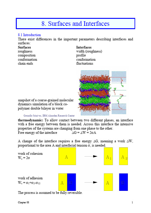
8. Surfaces and Interfaces8.1 IntroductionThere exist differences in the important parameters describing interfaces and surfaces:Surfaces Interfacesroughness composition conformation chain ends width (roughness) profile conformation fluctuationssnapshot of a coarse-grained moleculardynamics simulation of a block co-polymer double bilayer in waterGoundla Srinivas, IBM Almaden Research Centerthermodynamic: To allow contact between two different phases, an interface with a free energy between them is needed. Across this interface the intensive properties of the systems are changing from one phase to the other.Free energy of the interface ΔG = ΔW = 2σAA change of the interface requires a free energy ΔG, meaning a work ΔW, proportional to the area A and interfacial tension σ, is needed.work of cohesion W c = 2σwork of adhesion W c= σ1+σ2-σ12The process is assumed to be fully reversible.8.2 Polymer Surfaceair / vacuumpolymer surfacepolymer volume (bulk)Simple microscopic view: attractive forces between the atoms (spring-bead model) with force equilibrium in the volume, but missing partners at the surface→ attraction oriented towards the bulk→ surface tension / surface energy→ change of the structure at surfacea) Chain conformation in the vicinity of the surfaceComputer simulation: Structural properties of a dense polymer melt confined between two hard walls are investigated over a wide range of temperatures by dynamic Monte Carlo simulation using the bondfluctuation lattice model.The effect is present in a region close to the polymer surface. Deviation of the chain conformation is found in a region with an extension of ≈2R g .Baschnagel, Binder, Macromolecules 28, 6808 (1995)As the wall is further approached, the ability of the chains to reorient is progressively hindered, leading to an increase of R g|| and to a decrease of R g ⊥. Therefore the main effect of the wall is to reduce the orientational entropy of the polymers and to align them preferentially parallel to it.Experiments (GISANS): The samples consist of blend films of protonated and deuterated polystyrene (PS) spin coated onto glass substrates. A variation of the thickness of the blend films in a range of about 41 down to 0.66 times the radius of gyration R g of the chains in the bulk enables the determination of film thickness and confinement effects with the advanced scattering technique grazing incidence small angle neutron scattering (GISANS).The effect of the breaking of the translation symmetry by the presence of a surface is found in a more extended region of ≈8R g .Kraus et al., Europhys. Lett. 49, 210 (2000)The polymer molecule is altered in its conformation from an isotropic Gaussian chain (sphere) into an ellipsoidal shapechain segments are oriented in parallel to surfaceb) Chain end distribution Theory:Density of chain ends at the surface (de Gennes, 1992):φφρee N 2=with N length of chainφe number of ends at surfaceφ number of monomers per volume→ chain ends from a region 2R g are enriched in a layer of thickness d (typically 1-2 nm):N dae 2=ρ with segmental length aenrichment of chain ends at the surface due to entropic effects Experiments (NR): Mono-terminated polystyrenes (PS) are synthesized anionically to include a short perdeuteriostyrene sequence adjacent to the end groups for the purpose of selective contrast labeling of the end groups for neutron reflectivity (NR).The location of deuterium serves as a marker to indicate the location of the adjacent end group. Damped oscillatory end group concentration depth profiles at both the air and substrate interfaces are found. The periods of these oscillations correspond approximately to the polymer chain dimensions.contrast density depth profileKoberstein et al; Macromolecules 27,5341 (1994)c) Segment distribution in the vicinity of surfaceComputer simulation: Strong orientation of segments due to the breaking of the translational symmetry of the system by the presence of a surface. The effect is present in region close to surface only, with extension of ≈2R g.Experiments (Force balance): Strong modulation in the density in the vicinity of the surface (effect much more pronounced in case of a solid wall).transition region with significantly decreased densityd) Influence on the kineticsComputer simulation:At the polymer surface a very mobileand quasi-liquid layer is existing wellbelow a melting temperature T m. In thislayer the chain mobility is increased.at surface mobility in movement in parallel to the surface is increased in a thinlayer of thickness d (typically 2 nm)This behavior is similar to many crystal samples. The origin is the reduced number of entanglements at the surface.Experiments (FCS): Comparison of polymer diffusion, polyethyleneglycol (PEG), when adsorbed to a solid surface and in free solution(a) Flexible polymer chains that adsorb are nearly flat at dilute surface coverage (i.e., de Gennes pancake). The sticking energy for each segment is small, so no single segment is bound tightly, but the molecular sticking energy is large. (b) Diffusion coefficients (D) in dilute solution (blue circles) and at dilute coverage on a solid surface (red squares) plotted against the degree of polymerization (N) at 22°C.on surface: changed power law due to excluded volume statisticsDepending on the interaction between polymer and wall the mobility can by unchanged to bulk (neutral wall) or slowed down (attractive wall).How do polymer surfaces look in experiments?Examples:polystyrene machined titanium dual-acid-etched (DAE)titaniumSEMAFMNakamura et al, JDR 84, 515 (2005)Typically polymer surfaces are significantly smoother as compared to metal and metal oxide surfaces (independent of the surface treatment).PMDEGA after swelling in water vapor after 6 days storage in airZhong, PMB et al, Colloid. Polym. Sci. 289, 569 (2011)Homopolymer surfaces are only smooth with low surface roughness and good homogeneity if the homopolymer film is stable. If it is unstable the surface can roughen.If the polymer crystallizes a completely different polymer surface is observed. Due to the crystals present at the polymer surface, the surface roughness is significantly increased.8.3 Interface between polymerscase I: identical polymers A/A or compatible polymers A/B• interdiffusion of segments • adhesion • model of segment movementexample: PS/PS, PMMA/PMMA, PMMA/PVCcase II: incompatible polymers A/B• width of the interface in equilibrium • polymer-polymer interaction parameter (Flory-Huggins parameter) χexample: PS/PBrS, PS/PMMA, PS/PpMS, PS/PnBMAMathematical description of the interface:Rough interface j with mean z-coordinate set to zero and fluctuations in height z j (x)The rough interface can be replaced by an ensemble of smooth interfaces weighted by a probability density P j (φ)with a mean value ∫=dz z zP j j )(μand root-mean-square (rms) roughness ()∫−=dz z P z j j j )(22μσDifferent probability density function are possible and result in different interfaces: Normalized error-function (solid line) and hyperbolic-tangent (dashed line) have very similar refractive index profiles n j (z).Error function profile⎟⎟⎠⎞⎜⎜⎝⎛−−−+=++j j j j j j j z z erf n n n n z n σ222)(11 results from Gaussian probability density (μi =0) ⎟⎟⎠⎞⎜⎜⎝⎛−=222exp 21)(j jj z z P σσπand hyperbolic-tangent profile ⎟⎟⎠⎞⎜⎜⎝⎛−−−+=++j j j j j j j z z n n n n z n σπ32tanh 22)(11results from probability density (μi =0) ⎟⎟⎠⎞⎜⎜⎝⎛=−j jj z z P σπσπ32cosh 34)(2Both examples are based on symmetric probability functions, however, for real samples this symmetry is not ensured and thus asymmetric profiles can occur (e.g. polymer brush with exponential decay).a) Interface width of polymer interfacesComputer simulation (Monte-Carlo simulation by Binder, 1994):A symmetric binary mixture (polymer1, polymer2) below its critical temperature T c of unmixing is considered in a thin-film geometry confined between two parallel walls, where it is assumed that one wall prefers polymer1 and the other wall prefers polymer2. Then an interface between the coexisting unmixed phases is stabilized.with interface width χ6a L = yields rms-roughness πσ2L rms =only valid for smooth interfaces (σrmssmall) with qR g >1 and N →∞with segment length a scattering vector ()dq πλπ2sin 4=Θ=Not taking into account: - concentration dependence of χDifferent approximations in the framework of Mean Field theories:• Binder: expansion of free energy for φ=0.5 and N 1=N 2=N (with qR g >1 and χN>>1)()NaL 26−=χ• Brosetta: Integration of the quadratic gradient term in the vicinity of φ=0.5⎟⎠⎞⎜⎝⎛⎥⎦⎤⎢⎣⎡+−=21112ln 26N N aL χ• Stamm: minimization of the free energy using a "trial"-function⎟⎟⎠⎞⎜⎜⎝⎛⎥⎦⎤⎢⎣⎡+−=2121166N N aL πχ ⇒ It is possible to determine the polymer-polymer interaction parameter χ froma measurement of the interface width L, in case the degree of polymerization Nand the segment length a are known!• Frisch: modification of the profile on different length scales: deviation from the simple tanh-shapeb) entanglement density at the interface between two immiscible polymers The variation of entanglement density with interface width at an interface between two polymers is calculated using the relationships between chain packing and entanglement. The chain packing is obtained by the use of self-consistent mean-field techniques to calculate the average chain conformations within the interface region.calculated number of segmentsbetween entanglements as a functionof χassuming a bulk value of N e,typical for polystyrene, of 130Oslanec and Brown, Macromolecules 36, 5839 (2003)b) time dependent evolution of the interface widthHowever, all these models describe a time average and the final equilibrium interface. With experimental techniques it is possible to prepare interface between polymers far from equilibrium and to follow changes with time resolution.covering a large range of time and length scales the crossover between 4different regimes is observedt < τe: Rouse regimeτe < t < τf: Reptation regimeτf < t < τd: Blob movementτd < t: Fick diffusioncharacteristic power laws: tαRouse regime: α = 0.5Reptation regime: α = 0.25Fick Diffusion: α= 1.08.4 Rouse Model(P.E.Rouse 1953, extension B. Zimm 1956)The Rouse model describes the conformational dynamics of ideal chains. The main assumptions are: 1. no excluded volume interaction2. no hydrodynamic interactionTherefore one expects this model to work at Θ-condition or polymer melt condition.Polymers are interconnected objects with a large conformational entropy. As a consequence, the universal entropy-driven Rouse dynamics prevails at intermediate scales, where local potentials have ceased to be important and entanglements are not yet active. Key signature of the Rouse motion is the sublinear evolution of the segmental mean-square displacement2)(t2/1tr≈neutron spin echo (NSE) results on the single-chain dynamic structure factor: dynamics of poly(vinyl ethylene) on length scales covering Rouse dynamicsMean-square displacementof the protons, the solid linerepresents Rouse dynamicsRicher et al., Europhys. Lett., 66, 239(2004)Both molecular-dynamics (MD) simulations and MCT calculations on coarse-grained polymer models (bead and spring models)Bead-spring modelIn this model of a polymer molecule it consists of beads and springs forming a chain. The beads are hydrodynamics resistance sites that are dragged on by the suspending fluid. They also experience random Brownian forces caused by the thermal fluctuations in the fluid which are significant on the molecular scale. The spring is an entropic force pulling the adjacent beads together. In fact, the spring represents many monomer units that can coil and uncoil in response to the forces. This model is a reasonable representation of the polymer chain dynamics that actual polymer molecules undergo.8.5 Reptation Model(de Gennes, Doi, Edwards, 1971 + 1978)Reptation is the snake-like thermal motion of very long linear, entangled macromolecules in polymer melts or concentrated polymer solutions. It comprises:• entanglements with other chains hinder diffusion• each polymer chain is envisioned as occupying a tube of length L • movement of polymer chain is only possible within this fictive tube• special type of movement: diffusion only via movement of chain ends,keeping chain conformation unchangedtube diameter ddifferent types of movement:t < τe : no hindering in movement by tube (Rouse type movement)t = τe : density fluctuations within the chain are extended up to the length scale of the tube diameterτe < t < τf : polymer chain moves along the tubeτf < t < τd : chain starts to escape the tubet = τd : chain left the original tubet > τd : completely free movement of the chain with no remembering of the tubeExample:PE M w = 190k d = 49Å or PE M w = 17k d = 54ÅPS d ≈ 50ÅN R e , density ρ und temperature TInfluence on the interface profile:shown for different relative diffusion times t/t f 0.1 s mall →0.9 largeThe jump in the concentration profile is caused by the movement of the chain ends across the interface in the framework of the Reptation model.Attention: the profile needs to be convoluted with the tube diameter d8.6 Fick diffusionTranslation of the complete polymer chain is described as diffusion of the centerof masswith diffusion coefficient D Attention: different diffusion coefficients are existing D S self-diffusion coefficient (A moves in a matrix of A) D I inter-diffusions coefficient (A und B move with respect to each other) D T tracer-diffusion coefficient (marker T moves in matrix A)a) self-diffusion:Movement of chains in the identical environment → very difficult to detect experimentally, because no contrast between chain and environmentPossibility of marking individual chains (by deuteration or with fluorescent end-groups), but strictly this is a tracer experiment already Example: PS volume D S ≈4*10-14 cm 2/s thin film (300Å) D S ≈1.5*10-15 cm 2/s surface D S ≈9.3*10-16 cm 2/s⇒ slowing down of the diffusion due to the spatial confinementb) inter-diffusion:An interface between two polymers, which was prepared out of equilibrium (e.g. with the floating technique) is annealed above the glass transition temperature of both polymers→ broadening of the interface following the above arguments → late stages are caused by diffusion (t > τd )Experiment: X-ray- or neutron reflectivity measurementshydrogenated and deuterated polystyrene has been measured at 115 °C in-situ and in real time using NRdiffusion coefficientD = (1.7±0.2) × 10-17 cm 2/sBucknall et al., Macromolecules 32, 5453 (1999)• "fast-mode" theory B T B A A T A B I D N D N D ,,φφ+= • "slow-mode" theoryB T B A A T A B I D N D N D ,,111φφ+=Examples:Low molecular weight liquids D ≈10-6 cm 2/s polymers D ≈10-12-10-17 cm 2/s depending on temperaturec) tracer-diffusionusing small markers, e.g gold atoms in a well defined layered approachAnnealing the sample above the glass transition temperature of the polymer and probing the distances which the gold atoms had moved after defined times tReiter et al. Macromolecules 24, 1179 (1991)Dependence on molecular weight:Stamm et al., Macromolecules, 26, 2134 (1993)tracer-diffusions constant2−∝W T M D8.7 additional contributions to the interface widthIn addition to the width of the interface between two polymers which results from interdiffusion, contribution from other sources have to be taken into account. They arise from preparation: thickness variation of the filmwrinkles, dust particles, holes, impuritiesintrinsic: capillary wavesA capillary wave is a wave traveling along the phase boundary of a fluid, whose dynamics are dominated by the effects of surface tension. These waves are of thermal origin .Assuming a semi-infinite liquid with surface tension γLV a complex movement of the atoms makes a surface wavehaving a dispersion relation()g q q q LV rr r +=ργω32with ρ liquid density g Earth's accelerationSo thermal fluctuations cause a deviation from the ideal flat surface with an excess free energy density()()()()()Ζ⎥⎦⎤⎢⎣⎡ΖΔ+⎟⎠⎞⎜⎝⎛−Ζ∇+=Ζ∫∫22111d l P h A h fA L LV L exr r r γ ()()()()()Ζ⎥⎦⎤⎢⎣⎡Ζ+Ζ∇≈Ζ∫∫221d h P h A h f A L L LV L ex r r r γ yielding the height-height-autocorrelation function and power spectral density()Ζ=Ζr r c LV B q K Tk C 02)(πγ and 22214)(c LV LV B q q T k q L γγπ+=rwith K 0 modified Bessel function of zero ordercapillary waves can only be excited in an interval between λmin and λc for T>>0KA gravitation cut-off of the larges possible wavelength being excited isc c q πλ2=with LVc g q γρ=2 with the capillary length gLVργξ=being the lateral correlation length characteristic for the liquid (on the order of mm)and a short-range cut-off on the scale of the molecule diameter a is needed to avoid divergence of C(Ζ)a q 22maxmin ==πλ with a q π=maxExample: ethanol-vapor interface, σ=6.9 Åx-ray reflectivity and longitudinal diffuse scattering x-ray transverse diffuse scatteringSanyal et al.; Phys. Rev. Lett. 66, 628 (1991)Attention: in case of interfaces instead of surfaces the surface tension γLV is replaced by the interface tension γLL which is orders of magnitude smaller than the surface tension→ contribution of capillary waves to rms-roughness of interface increasedExample: Direct visual observation of thermal capillary waves at the free liquid-gas interface in a phase-separated colloid-polymer mixture imaged with laser scanning confocal microscopy (LSCM) at four different state points approaching the critical point(2004) each image is 17.5 μm by 85 μmAarts et al. Science 304,847Simple liquid → polymer:For highly viscous liquids and polymer melts the capillary waves are overdamped, their amplitude reduced.While, in general, both damped and propagating modes exist, for highly viscous polymers all modes are overdamped, which can be characterized solely by relaxation times τ.physical meaning of the over-damped relaxation timeconstantSinha, University of CaliforniaRoughness measurements are time averaged and cannot reveal the dynamic behavior of the waves.→ Need to probe the dynamics!Experiments: XPCSExample: capillary wave dynamics on glycerol surfaces investigated with XPCS performed at grazing anglesnormalized time correlation function22)()()()(ttt I t I t I g ττ+=described by exponential behavior1exp )(002+⎟⎟⎠⎞⎜⎜⎝⎛−=τττg g→ relaxation times τSeydel et al., Phys. Rev. B 63, 073409 (2001)The capillary wave is identified by its wave vector q and complex frequencyΓ+=i f p ωwhere the real part reflects the propagation frequency and the imaginary part the damping.At the transition from propagating to overdamped behavior f becomes purely imaginary; i.e., ωp =0.The transition from propagating (inelastic) to overdamped (quasielastic) behavior takes place at critical wave vector254ηργLV c q =with surface tension γLV , the dynamic viscosity η, and the density ρ of the polymerExample: Mixture of water and glycerol with 65% weight concentration of glycerolMadsen et al., Phys. Rev. Lett. 92, 096104 (2004)propagation frequency ωp (circles) and the dampingconstant Γ (squares) for the water -glycerol mixture at (a)30 °C and (b) 12 °C.8.8 Thin Film Preparation Techniques a) Solution-castingpreparation of thick polymer films (thickness from 100 nm to several μm)• polymer solution deposited on top of a horizontally oriented substrate• cover full substrate to have chance for uniform film if liquid is not spreading • solvent evaporates under controlled condition (T, p, atmosphere) → a solid film remains on the substrate→ allows for slow drying: films close to equilibrium can be preparedOn the scale of the capillary length the film at the substrate edges differs from the average film.Problems occur in case of pinning effects. If the contact line gets pinned during drying, no homogenous film is formed.Example: ternary blend PS, P αMS and PI cast from toluenePanagiotou, PhD Thesis TU Munich (2004)For complex fluids (highly viscous polymer solutions), the morphology is not determined by the evaporation process, the "coffee stain" effect but essentially by the capillary instabilities.Using the appropriate couple of polymer/solvent, a outward, inward or a lack of Marangoni flow in the droplets, leading to the formation of a rim, a drop or a uniform film, respectively, occurs.b) Spin-coatingpreparation of thin polymer films with thicknesses from 1 to 1000 nm• prepare polymer solution with desired concentration c • cover substrate entirely with polymer solution• select acceleration profile and spinning parameters (time, rotational speed) • start spin-coater after defined wait time → a solid film remains on the substrate→ due to non-equilibrium the film can have enrichment or lateral structuresDepending on rotational speed ω, concentration c, molecular weight Mw and apersonal parameter (wait time, person, machine)Attention: change in slope at entanglement concentration of solutionRuderer, PMB, Chem.Phys.Chem. 10, 664 (2009)Spin-coating is a complicated non-equilibrium processTheoretical description in the framework of a 3-step model (Lawrence, 1988) 1. step – start phasedeposition of solution with C 0 → strong height variationsacceleration of the substrate → most of the solution is flung-off the substrate → film thickness ≈100 μmEnd: Homogeneous film with thickness h 0 with concentration C 0 2. step – mass reduction by conventionevaporation can be neglected in comparison with the flow of solution towards to substrate edges → change of film thickness by convection2/102020341)(−⎟⎟⎠⎞⎜⎜⎝⎛+=t h h t h ηρω 3. step – evaporation of solvent through film surfaceevaporation rate of solvent larger than change in thickness by convection at a film thickness h w → mass reduction only by solvent evaporation, no polymer can leave the substrate anymore → dry, solid film remains()0,1s w f h h φ−=With the initial amount of solvent φs,0Polymer surface depends on the used solvent and on the spin-coating parameters:I: problems with solvents which have very high evaporation rate: → formation of skin on solution surface→ elastic film surface has a changed flow field of the confined polymer solution → hydrodynamic instabilities→ resulting lateral structures which have a star-shape with the center in the center of rotationII: problems with solvents which are hygroscopic and attract water from the surrounding, but are non miscible with water:→ demixing of both components (solvent and water) gives rise to lateral structuresMüller-Buschbaum et al.; Macromolecules 31, 3686 (1998)c) Floating-techniquepreparation of single and multiple polymer films (on non-wetable substrates)Schindler, Diploma Thesis TU Munich (2010)• scratch film with scalpel at 2 mm from substrate edge • put substrate into float box (tilt angle optimal at 10-15°) • add 2-3 drops of deionized water per second • remove substrate after film had decoupled• put second substrate with larger tilt angle into the water • fix polymer film on upper edge of this second substrate • remove water with 2-3 drops/sec • dry films (e.g. 4 h at 50°C)→ typically the needed time is 3-6 hours depending on the M w and film thickness→ not possible for all film thickness (thinner films are more difficult, integer number of R g can work), not possible for heat treated filmsProblems occur in case of wrinkle formation, incorporation of dust particles or trapping of water.Example: freely floating polymer film, tens of nanometers in thickness, wrinkles under the capillary force exerted by a drop of water placed on its surfaceThe wrinkling pattern is characterized by the number and length of the wrinkles.The PS film thickness h was varied from 31 to 233 nm. As the film is made thicker, the number of wrinkles N decreases (there are 111, 68, 49, and 31 wrinkles in these images).Huang et al.; Science 317, 650 (2007)d) Adsorption from solutiondeposition of single molecules, thin layers or thick films from solution with a controlled concentrationSketch:Adsorption is usually described through isotherms, that is, the amount of adsorbate on the adsorbent as a function of its pressure (if gas) or concentration (if liquid) at constant temperature.Isotherms are described bydifferent models:Langmuir isotherm (red) andBET isotherm (green)Computer simulation:Adsorption and self-assembly of linear polymers on smooth surfaces are studied using coarse-grained, bead-spring molecular models and Langevin dynamics computer simulations. The aim is to gain insight on atomic-force microscopy images of polymer films on mica surfaces, adsorbed from dilute solution following a good-solvent to bad-solvent quenching procedure.Chremos et al., Soft Matter5, 637 (2009)Molecular Weight Competition: Upon initial mixing of a formulation, all chains attempt to adsorb on a surface. For adsorbing homopolymers, thermodynamics dictates a preference for adsorption of long chains, and so short chains, originally adsorbed, are displaced form the surface at longer times.Santore+ Fu, Macromolecules 30, 8516 (1997)Fu + Santore, Macromolecules 31, 7014 (1998) Large scale industrial applications involving substantial quantities of complex fluids such as paints, inks, and coatings employ water soluble polymers with a broad distribution of molecular weights: The likelihood that some fraction of the added chains impart the desired interfacial properties means that changes in molecular weight distribution from batch to batch can dramatically impact the properties of a formulation.Experiments: Adsorption of polymers is very common in case of polyeletrolytes and used to build up multi-layers.Layer-by-Layer (LBL) assembly: fabrication of multilayers by consecutive adsorption of polyanions and polycationsDecher et al.; Science 277, 1232 (1997)Fine-tuning the film thickness by ionic strength (addition of salt yields thicker layers; polyanion from salt, polycation from pure water)Decher + Schmitt, Progr. Colloid Polym. Sci. 89, 160 (1992) A small list of polyions already used for multilayer fabrication:e) Spray coatingdeposition of thick films from solution with a controlled concentration, depending on deposition conditions (wet droplets = spraying, dry polymer = airbrush)control parameters: number of depositions, deposition time, solvent, polymer concentration, distance nozzle-surface。

a r X i v :c o n d -m a t /9503139v 1 27 M a r 1995Singularity of the density of states in the two-dimensional Hubbard model from finitesize scaling of Yang-Lee zerosE.Abraham 1,I.M.Barbour 2,P.H.Cullen 1,E.G.Klepfish 3,E.R.Pike 3and Sarben Sarkar 31Department of Physics,Heriot-Watt University,Edinburgh EH144AS,UK 2Department of Physics,University of Glasgow,Glasgow G128QQ,UK 3Department of Physics,King’s College London,London WC2R 2LS,UK(February 6,2008)A finite size scaling is applied to the Yang-Lee zeros of the grand canonical partition function for the 2-D Hubbard model in the complex chemical potential plane.The logarithmic scaling of the imaginary part of the zeros with the system size indicates a singular dependence of the carrier density on the chemical potential.Our analysis points to a second-order phase transition with critical exponent 12±1transition controlled by the chemical potential.As in order-disorder transitions,one would expect a symmetry breaking signalled by an order parameter.In this model,the particle-hole symmetry is broken by introducing an “external field”which causes the particle density to be-come non-zero.Furthermore,the possibility of the free energy having a singularity at some finite value of the chemical potential is not excluded:in fact it can be a transition indicated by a divergence of the correlation length.A singularity of the free energy at finite “exter-nal field”was found in finite-temperature lattice QCD by using theYang-Leeanalysisforthechiral phase tran-sition [14].A possible scenario for such a transition at finite chemical potential,is one in which the particle den-sity consists of two components derived from the regular and singular parts of the free energy.Since we are dealing with a grand canonical ensemble,the particle number can be calculated for a given chem-ical potential as opposed to constraining the chemical potential by a fixed particle number.Hence the chem-ical potential can be thought of as an external field for exploring the behaviour of the free energy.From the mi-croscopic point of view,the critical values of the chemical potential are associated with singularities of the density of states.Transitions related to the singularity of the density of states are known as Lifshitz transitions [15].In metals these transitions only take place at zero tem-perature,while at finite temperatures the singularities are rounded.However,for a small ratio of temperature to the deviation from the critical values of the chemical potential,the singularity can be traced even at finite tem-perature.Lifshitz transitions may result from topological changes of the Fermi surface,and may occur inside the Brillouin zone as well as on its boundaries [16].In the case of strongly correlated electron systems the shape of the Fermi surface is indeed affected,which in turn may lead to an extension of the Lifshitz-type singularities into the finite-temperature regime.In relating the macroscopic quantity of the carrier den-sity to the density of quasiparticle states,we assumed the validity of a single particle excitation picture.Whether strong correlations completely distort this description is beyond the scope of the current study.However,the iden-tification of the criticality using the Yang-Lee analysis,remains valid even if collective excitations prevail.The paper is organised as follows.In Section 2we out-line the essentials of the computational technique used to simulate the grand canonical partition function and present its expansion as a polynomial in the fugacity vari-able.In Section 3we present the Yang-Lee zeros of the partition function calculated on 62–102lattices and high-light their qualitative differences from the 42lattice.In Section 4we analyse the finite size scaling of the Yang-Lee zeros and compare it to the real-space renormaliza-tion group prediction for a second-order phase transition.Finally,in Section 5we present a summary of our resultsand an outlook for future work.II.SIMULATION ALGORITHM AND FUGACITY EXPANSION OF THE GRAND CANONICALPARTITION FUNCTIONThe model we are studying in this work is a two-dimensional single-band Hubbard HamiltonianˆH=−t <i,j>,σc †i,σc j,σ+U i n i +−12 −µi(n i ++n i −)(1)where the i,j denote the nearest neighbour spatial lat-tice sites,σis the spin degree of freedom and n iσis theelectron number operator c †iσc iσ.The constants t and U correspond to the hopping parameter and the on-site Coulomb repulsion respectively.The chemical potential µis introduced such that µ=0corresponds to half-filling,i.e.the actual chemical potential is shifted from µto µ−U412.(5)This transformation enables one to integrate out the fermionic degrees of freedom and the resulting partition function is written as an ensemble average of a product of two determinantsZ ={s i,l =±1}˜z = {s i,l =±1}det(M +)det(M −)(6)such thatM ±=I +P ± =I +n τ l =1B ±l(7)where the matrices B ±l are defined asB ±l =e −(±dtV )e −dtK e dtµ(8)with V ij =δij s i,l and K ij =1if i,j are nearestneigh-boursand Kij=0otherwise.The matrices in (7)and (8)are of size (n x n y )×(n x n y ),corresponding to the spatial size of the lattice.The expectation value of a physical observable at chemical potential µ,<O >µ,is given by<O >µ=O ˜z (µ){s i,l =±1}˜z (µ,{s i,l })(9)where the sum over the configurations of Ising fields isdenoted by an integral.Since ˜z (µ)is not positive definite for Re(µ)=0we weight the ensemble of configurations by the absolute value of ˜z (µ)at some µ=µ0.Thus<O >µ= O ˜z (µ)˜z (µ)|˜z (µ0)|µ0|˜z (µ0)|µ0(10)The partition function Z (µ)is given byZ (µ)∝˜z (µ)N c˜z (µ0)|˜z (µ0)|×e µβ+e −µβ−e µ0β−e −µ0βn (16)When the average sign is near unity,it is safe to as-sume that the lattice configurations reflect accurately thequantum degrees of freedom.Following Blankenbecler et al.[1]the diagonal matrix elements of the equal-time Green’s operator G ±=(I +P ±)−1accurately describe the fermion density on a given configuration.In this regime the adiabatic approximation,which is the basis of the finite-temperature algorithm,is valid.The situa-tion differs strongly when the average sign becomes small.We are in this case sampling positive and negative ˜z (µ0)configurations with almost equal probability since the ac-ceptance criterion depends only on the absolute value of ˜z (µ0).In the simulations of the HSfields the situation is dif-ferent from the case of fermions interacting with dynam-ical bosonfields presented in Ref.[1].The auxilary HS fields do not have a kinetic energy term in the bosonic action which would suppress their rapidfluctuations and hence recover the adiabaticity.From the previous sim-ulations on a42lattice[3]we know that avoiding the sign problem,by updating at half-filling,results in high uncontrolledfluctuations of the expansion coefficients for the statistical weight,thus severely limiting the range of validity of the expansion.It is therefore important to obtain the partition function for the widest range ofµ0 and observe the persistence of the hierarchy of the ex-pansion coefficients of Z.An error analysis is required to establish the Gaussian distribution of the simulated observables.We present in the following section results of the bootstrap analysis[17]performed on our data for several values ofµ0.III.TEMPERATURE AND LATTICE-SIZEDEPENDENCE OF THE YANG-LEE ZEROS The simulations were performed in the intermediate on-site repulsion regime U=4t forβ=5,6,7.5on lat-tices42,62,82and forβ=5,6on a102lattice.The ex-pansion coefficients given by eqn.(14)are obtained with relatively small errors and exhibit clear Gaussian distri-bution over the ensemble.This behaviour was recorded for a wide range ofµ0which makes our simulations reli-able in spite of the sign problem.In Fig.1(a-c)we present typical distributions of thefirst coefficients correspond-ing to n=1−7in eqn.(14)(normalized with respect to the zeroth power coefficient)forβ=5−7.5for differ-entµ0.The coefficients are obtained using the bootstrap method on over10000configurations forβ=5increasing to over30000forβ=7.5.In spite of different values of the average sign in these simulations,the coefficients of the expansion(16)indicate good correspondence between coefficients obtained with different values of the update chemical potentialµ0:the normalized coefficients taken from differentµ0values and equal power of the expansion variable correspond within the statistical error estimated using the bootstrap analysis.(To compare these coeffi-cients we had to shift the expansion by2coshµ0β.)We also performed a bootstrap analysis of the zeros in theµplane which shows clear Gaussian distribution of their real and imaginary parts(see Fig.2).In addition, we observe overlapping results(i.e.same zeros)obtained with different values ofµ0.The distribution of Yang-Lee zeros in the complexµ-plane is presented in Fig.3(a-c)for the zeros nearest to the real axis.We observe a gradual decrease of the imaginary part as the lattice size increases.The quantitative analysis of this behaviour is discussed in the next section.The critical domain can be identified by the behaviour of the density of Yang-Lee zeros’in the positive half-plane of the fugacity.We expect tofind that this density is tem-perature and volume dependent as the system approaches the phase transition.If the temperature is much higher than the critical temperature,the zeros stay far from the positive real axis as it happens in the high-temperature limit of the one-dimensional Ising model(T c=0)in which,forβ=0,the points of singularity of the free energy lie at fugacity value−1.As the temperature de-creases we expect the zeros to migrate to the positive half-plane with their density,in this region,increasing with the system’s volume.Figures4(a-c)show the number N(θ)of zeros in the sector(0,θ)as a function of the angleθ.The zeros shown in thesefigures are those presented in Fig.3(a-c)in the chemical potential plane with other zeros lying further from the positive real half-axis added in.We included only the zeros having absolute value less than one which we are able to do because if y i is a zero in the fugacity plane,so is1/y i.The errors are shown where they were estimated using the bootstrap analysis(see Fig.2).Forβ=5,even for the largest simulated lattice102, all the zeros are in the negative half-plane.We notice a gradual movement of the pattern of the zeros towards the smallerθvalues with an increasing density of the zeros nearθ=πIV.FINITE SIZE SCALING AND THESINGULARITY OF THE DENSITY OF STATESAs a starting point for thefinite size analysis of theYang-Lee singularities we recall the scaling hypothesis forthe partition function singularities in the critical domain[11].Following this hypothesis,for a change of scale ofthe linear dimension LLL→−1),˜µ=(1−µT cδ(23)Following the real-space renormalization group treatmentof Ref.[11]and assuming that the change of scaleλisa continuous parameter,the exponentαθis related tothe critical exponentνof the correlation length asαθ=1ξ(θλ)=ξ(θ)αθwe obtain ξ∼|θ|−1|θ|ναµ)(26)where θλhas been scaled to ±1and ˜µλexpressed in terms of ˜µand θ.Differentiating this equation with respect to ˜µyields:<n >sing =(−θ)ν(d −αµ)∂F sing (X,Y )ν(d −αµ)singinto the ar-gument Y =˜µαµ(28)which defines the critical exponent 1αµin terms of the scaling exponent αµof the Yang-Lee zeros.Fig.5presents the scaling of the imaginary part of the µzeros for different values of the temperature.The linear regression slope of the logarithm of the imaginary part of the zeros plotted against the logarithm of the inverse lin-ear dimension of the simulation volume,increases when the temperature decreases from β=5to β=6.The re-sults of β=7.5correspond to αµ=1.3within the errors of the zeros as the simulation volume increases from 62to 82.As it is seen from Fig.3,we can trace zeros with similar real part (Re (µ1)≈0.7which is also consistentwith the critical value of the chemical potential given in Ref.[22])as the lattice size increases,which allows us to examine only the scaling of the imaginary part.Table 1presents the values of αµand 1αµδ0.5±0.0560.5±0.21.3±0.3∂µ,as a function ofthe chemical potential on an 82lattice.The location of the peaks of the susceptibility,rounded by the finite size effects,is in good agreement with the distribution of the real part of the Yang-Lee zeros in the complex µ-plane (see Fig.3)which is particularly evident in the β=7.5simulations (Fig.4(c)).The contribution of each zero to the susceptibility can be singled out by expressing the free energy as:F =2n x n yi =1(y −y i )(29)where y is the fugacity variable and y i is the correspond-ing zero of the partition function.The dotted lines on these plots correspond to the contribution of the nearby zeros while the full polynomial contribution is given by the solid lines.We see that the developing singularities are indeed governed by the zeros closest to the real axis.The sharpening of the singularity as the temperature de-creases is also in accordance with the dependence of the distribution of the zeros on the temperature.The singularities of the free energy and its derivative with respect to the chemical potential,can be related to the quasiparticle density of states.To do this we assume that single particle excitations accurately represent the spectrum of the system.The relationship between the average particle density and the density of states ρ(ω)is given by<n >=∞dω1dµ=ρsing (µ)∝1δ−1(32)and hence the rate of divergence of the density of states.As in the case of Lifshitz transitions the singularity of the particle number is rounded at finite temperature.However,for sufficiently low temperatures,the singular-ity of the density of states remains manifest in the free energy,the average particle density,and particle suscep-tibility [15].The regular part of the density of states does not contribute to the criticality,so we can concentrate on the singular part only.Consider a behaviour of the typedensity of states diverging as the−1ρsing(ω)∝(ω−µc)1δ.(33)with the valueδfor the particle number governed by thedivergence of the density of states(at low temperatures)in spite of thefinite-temperature rounding of the singu-larity itself.This rounding of the singularity is indeedreflected in the difference between the values ofαµatβ=5andβ=6.V.DISCUSSION AND OUTLOOKWe note that in ourfinite size scaling analysis we donot include logarithmic corrections.In particular,thesecorrections may prove significant when taking into ac-count the fact that we are dealing with a two-dimensionalsystem in which the pattern of the phase transition islikely to be of Kosterlitz-Thouless type[23].The loga-rithmic corrections to the scaling laws have been provenessential in a recent work of Kenna and Irving[24].In-clusion of these corrections would allow us to obtain thecritical exponents with higher accuracy.However,suchanalysis would require simulations on even larger lattices.The linearfits for the logarithmic scaling and the criti-cal exponents obtained,are to be viewed as approximatevalues reflecting the general behaviour of the Yang-Leezeros as the temperature and lattice size are varied.Al-though the bootstrap analysis provided us with accurateestimates of the statistical error on the values of the ex-pansion coefficients and the Yang-Lee zeros,the smallnumber of zeros obtained with sufficient accuracy doesnot allow us to claim higher precision for the critical ex-ponents on the basis of more elaboratefittings of the scal-ing behaviour.Thefinite-size effects may still be signifi-cant,especially as the simulation temperature decreases,thus affecting the scaling of the Yang-Lee zeros with thesystem rger lattice simulations will therefore berequired for an accurate evaluation of the critical expo-nent for the particle density and the density of states.Nevertheless,the onset of a singularity atfinite temper-ature,and its persistence as the lattice size increases,areevident.The estimate of the critical exponent for the diver-gence rate of the density of states of the quasiparticleexcitation spectrum is particularly relevant to the highT c superconductivity scenario based on the van Hove sin-gularities[25],[26],[27].It is emphasized in Ref.[25]thatthe logarithmic singularity of a two-dimensional electrongas can,due to electronic correlations,turn into a power-law divergence resulting in an extended saddle point atthe lattice momenta(π,0)and(0,π).In the case of the14.I.M.Barbour,A.J.Bell and E.G.Klepfish,Nucl.Phys.B389,285(1993).15.I.M.Lifshitz,JETP38,1569(1960).16.A.A.Abrikosov,Fundamentals of the Theory ofMetals North-Holland(1988).17.P.Hall,The Bootstrap and Edgeworth expansion,Springer(1992).18.S.R.White et al.,Phys.Rev.B40,506(1989).19.J.E.Hirsch,Phys.Rev.B28,4059(1983).20.M.Suzuki,Prog.Theor.Phys.56,1454(1976).21.A.Moreo, D.Scalapino and E.Dagotto,Phys.Rev.B43,11442(1991).22.N.Furukawa and M.Imada,J.Phys.Soc.Japan61,3331(1992).23.J.Kosterlitz and D.Thouless,J.Phys.C6,1181(1973);J.Kosterlitz,J.Phys.C7,1046(1974).24.R.Kenna and A.C.Irving,unpublished.25.K.Gofron et al.,Phys.Rev.Lett.73,3302(1994).26.D.M.Newns,P.C.Pattnaik and C.C.Tsuei,Phys.Rev.B43,3075(1991);D.M.Newns et al.,Phys.Rev.Lett.24,1264(1992);D.M.Newns et al.,Phys.Rev.Lett.73,1264(1994).27.E.Dagotto,A.Nazarenko and A.Moreo,Phys.Rev.Lett.74,310(1995).28.A.A.Abrikosov,J.C.Campuzano and K.Gofron,Physica(Amsterdam)214C,73(1993).29.D.S.Dessau et al.,Phys.Rev.Lett.71,2781(1993);D.M.King et al.,Phys.Rev.Lett.73,3298(1994);P.Aebi et al.,Phys.Rev.Lett.72,2757(1994).30.E.Dagotto, A.Nazarenko and M.Boninsegni,Phys.Rev.Lett.73,728(1994).31.N.Bulut,D.J.Scalapino and S.R.White,Phys.Rev.Lett.73,748(1994).32.S.R.White,Phys.Rev.B44,4670(1991);M.Veki´c and S.R.White,Phys.Rev.B47,1160 (1993).33.C.E.Creffield,E.G.Klepfish,E.R.Pike and SarbenSarkar,unpublished.Figure CaptionsFigure1Bootstrap distribution of normalized coefficients for ex-pansion(14)at different update chemical potentialµ0for an82lattice.The corresponding power of expansion is indicated in the topfigure.(a)β=5,(b)β=6,(c)β=7.5.Figure2Bootstrap distributions for the Yang-Lee zeros in the complexµplane closest to the real axis.(a)102lat-tice atβ=5,(b)102lattice atβ=6,(c)82lattice at β=7.5.Figure3Yang-Lee zeros in the complexµplane closest to the real axis.(a)β=5,(b)β=6,(c)β=7.5.The correspond-ing lattice size is shown in the top right-hand corner. Figure4Angular distribution of the Yang-Lee zeros in the com-plex fugacity plane Error bars are drawn where esti-mated.(a)β=5,(b)β=6,(c)β=7.5.Figure5Scaling of the imaginary part ofµ1(Re(µ1)≈=0.7)as a function of lattice size.αm u indicates the thefit of the logarithmic scaling.Figure6Electronic susceptibility as a function of chemical poten-tial for an82lattice.The solid line represents the con-tribution of all the2n x n y zeros and the dotted line the contribution of the six zeros nearest to the real-µaxis.(a)β=5,(b)β=6,(c)β=7.5.。

岩土巨人介绍Ronald F. Scott加州理工学院教授1929– 2005 (2)Karl von Terzaghi (5)William John Macquorn Rankine(土力学学中的朗肯土压力理论的缔造者) (9)Arthur Casagrande (11)教授1929– 2005Ronald Fraser Scott, the Dotty and Dick Hayman Professor of Engineering, Emeritus, died on August 16, 2005. He was 76. An internationally acclaimed expert in soil mechanics and foundation engineering—or geotechnical engineering as it is now known—his research interests included the basic properties of soils and how they deform, the dynamics of landslides, the behavior of soil in earthquakes, the physical chemistry and mechanics of ocean-bottom soil, the physics of the freezing and thawing processes in soils, and the properties of the moon’s surface.Scott was born in London and grew up in Perth, Scotland. After ga ining a bachelor’s degree in civil engineering from Glasgow University in 1951 and an ScD in civil engineering (soil mechanics) from MIT in 1955, he worked with the U.S. Army Corps of Engineers on the construction of pavements on permafrost in Greenland, and with consulting engineers Racey, McCallum and Associates in Toronto, before joining Caltech as an assistant professor of civil engineering in 1958. Rising through the ranks, he became the Hayman Professor in 1987, and retired in 1998.On February 11, a memorial gathering in Scott’s honor was hosted by Norman Brooks (PhD ’54), Irvine Professor of Environmental and Civil Engineering, Emeritus. Caltech provost and professor of civil engineering and applied mechanics Paul Jennings, (MS ’60, PhD ’63, who to ok one of Scott’s soil mechanics classes as a graduate student), told the gathering that Scott had taken on a challenging field. ―As engineering materials, soils are simply not nice,‖ he said. ―They are complicated two-phase media, composed of a porous collection of particles and a fluid in thepores, typically water. As such, soils are kind of noneverything—nonlinear, nonelastic,nonhomogeneous, nonisotropic and therefore from the viewpoint of solid mechanics, noneasy.‖ But, he said, Scott was a Caltech type of engineer—half engineer, half scientist—who developed engineering tools and approaches based on a rigorous understanding of the fundamental mechanics involved.―This real-world messiness of soils translates to the classroom,‖ Jennings added. ―Around the country, soil mechanics courses are often not popular because the material resists the elegant mathematical simplifications that take one so far in other materials, like metals. Ron’s courses were different; they were well-appreciated and popular because he met the challenges of soil complexity head-on in his unique and interesting way.‖When he began teaching, there were no textbooks that suited Scott’s rigorous scientific approach based on the mathematical principles of solid and fluid mechanics, so he wrote several of his own, including Principles of Soil Mechanics (1963) and Foundation Analysis (1981).―His understanding of the theoretical issues was profound,‖ said James Knowles, the Kenan, Jr., Professor and Professor of Applied Mechanics, Eme ritus, ―but his work was always motivated by real-world problems and needs, and he accumulated much practical experience by consulting on such problems as landslides and soil liquefaction.‖ Living as he did in a region highly prone to landslides and earthq uakes, Scott’s expertise was called upon many times by consulting firms and government agencies. He was an advisor during the investigations that followed the Baldwin Hills Dam failure in Los Angeles in 1963 and the Bluebird Canyon landslide in Laguna Beach in 1978, and worked with Fred Raichlen, professor of civil and mechanical engineering, emeritus, to design the foundations of submarine wastewater outfalls to withstand earthquakes and high waves.Scott pioneered the use of centrifuges in soil dynamics, recognizing that the mechanical properties of soils depend on the pressures to which they’re subjected. The soil at the bottom of a large earthen dam, for example, is under an enormous amount of pressure from the weight of the soil above and around it. Laboratory-sized scale models, using much less soil, can’t reproduce this. Scott’s solution was to spin the model in a large centrifuge to achieve forces 50 to 100 times the acceleration due to gravity. His centrifuge also incorporated a computer-controlled shaking table that could model the intense motion of soil during an earthquake. ―This technology has been copied and refined at other labs around the world, but Ron was the originator,‖ said John Hall, professor of civil engineering and dean of students.In the 1960s, Scott’s expertise made him the ideal person to evaluate whether the surface of the moon would be safe to walk on. At the time, many people thought it was covered in a deep layer of fine dust, like talc, that wouldn’t support the weight of a human. As a principal investigator for Surveyors 3 and 7, two unmanned craft preparing the way for the Apollo 11 manned landing, hedesigned an instrument to examine the structure and load-bearing strength of the lunar soil.Scott’s box-shaped, claw-mou thed scoop, or ―soil mechanics surface sampler,‖ as NASA called it, was attached to a telescopic arm and could be moved around and lifted up and down by radio signals from Earth. The scoop could dig trenches, scrape up soil, and even lift large clods and drop them to break up the lumps. And by filling the scoop with soil and compressing it, Scott and JPL engineer Floyd Roberson could estimate its bearing strength.Surveyor 3 landed on the moon in 1967, and ―for the next two weeks,‖ Scott later wrote in th e February 1970 issue of E&S, ―Floyd and I happily and sleeplessly played with the lunar surface soil on the inside surface of a 650-foot-diameter crater.‖ The moon’s surface, they concluded, was like damp sand, and safe to walk on.When the time came for the manned landing, Scott waited anxiously on July 20, 1969, as Neil Armstrong climbed down the ladder of the lunar module Eagle. Everyone remembers Armstrong’s first words, ―That’s one small step for man, one giant leap for mankind,‖ but not many rememb er what he said next: ―I sink in about an eighth of an inch. I’ve left a print on the surface.‖ Those were the words Scott wanted to hear.There’s a postcript to this story. In November 1969, Apollo 12’s module landed close to Surveyor 3, and Charles Conrad and Alan Bean walked over to take a look at it. Conrad cut off the scoop and brought it back to Earth in two Teflon bags. Scott was present when the bags were opened. ―If I had known I would see it again,‖ Scott told E&S, ―I would have left the scoop c ompletely packed with lunar soil.‖The two V iking spacecraft that landed on Mars in 1976 also needed soil scoops, and again, Scott worked on those. As mentioned in E&S, No. 4, 2005, some of the soil collected by the scoops was used in a life-detection experiment designed by another Caltech faculty member, Norman Horowitz, who died shortly before Scott.Former students and colleagues at the memorial gathering mentioned Scott’s high standards. ―He did not tolerate sloppy or inaccurate research or engineer ing,‖ said Raichlen, ―and he had little patience with others who fell into that category.‖ A ―fiercely independent thinker,‖ Scott ―valued academic integrity above all else,‖ said John Ting, MS ’76, professor and dean of engineering at the University of Ma ssachusetts at Lowell. ―It wasn’t about the size of the research group, or the amount of funding—it was about the purity of the academic pursuit, and asking and then answering the key questions in the most elegant (and often the least expensive) way.‖ Two of Scott’s former graduate students, Hon-Yim Ko (MS ’63, PhD ’66), Murphy Professor ofEngineering at the University of Colorado at Boulder, and Thiam-Soon Tan (MS ’82, PhD ’86), associate professor of civil engineering at the National University of Singapore, also paid tribute to their mentor and friend. Many of the speakers remarked on Scott’s wit, his wry sense of humor, and his infectious laugh.Scott cultivated a love of literature and was an omnivorous reader, said his son, Grant, a professor of English at Muhlenberg College in Pennsylvania. And in a fitting tribute to his soil-engineer father, he said ―My father loved words—especially puns—where there was slippage in the slope of language, perhaps a kind of liquefaction where two letters supporting a dam of meaning gave way or there was a semantic friction or failure. He liked to see words collapse into other words, and watch as a seismic shift altered the landscape of a sentence.‖Scott was elected to the National Academy of Engineering in 1974. His awards included the American Society of Civil Engineers’ Walter L. Huber Civil Engineering Research Prize in 1969, the Norman Medal in 1972, and the Thomas A. Middlebrooks A ward in 1982. He was also selected to be the ASCE’s Terzaghi lecturer in 1983, and the British Geotechnical Society’s Rankine lecturer in 1987. Considered to be the two highest honors in Scott’s field, they are rarely awarded to a single person.He is survived by Pamela, his wife of over 46 years, sons Grant, Craig, and Rod, and seven grandchildren.可惜加州理工如今找不到几个教授再研究这个了，这个学科也湮灭在大牛的谈笑风生中了。

a r X i v :0707.3472v 1 [c o n d -m a t .s t a t -m e c h ] 24 J u l 2007Noname manuscript No.(will be inserted by the editor)This work was supported in part by a Grant-in-Aid for Scientific Research from Japan Society for the Promotion of Science.N i X i −¯X2,¯X=1NX 2− X 2 2 ,(9)which can reflect how large the skeleton size fluctuates.If the models un-dergo a collapsing transition,we can see ananomalous peak in C X 2at the transition point.We plot C X 2versus b in Figs.6(a)and 6(b),which were obtained in model 1and model 2,respectively.model N(ℓ,m)b(col)X2colmin X2colmaxb(smo)X2smominX2smomax23602(36,6) 2.652123 2.64140205 26402(48,8) 2.5860175 2.62210330 212102(66,11) 2.58100300 2.62400600 222502(90,15) 2.59190500 2.616801000N(S2− S2 )2 ,(14)which is the variance of S2.C S2of model2can be obtained by replacing Nby N′in Eq.(14).Just as C X2that reflects the collapsing transition,C S2 can also reflect the surfacefluctuation transition through its anomalous be-havior.Figures11(a)and11(b)show C S2versus b of model1and model2,respectively.The curves on thefigures were obtained also by the multihis-togram reweighting technique.Wefind an anomalous peak in C S2of bothmodels in Figs.11(a)and11(b).The peak values increase with increasing N(N′)and,therefore this indicates the existence of phase transition in both models.In order to see the order of the surfacefluctuation transition,we showin Fig.11(c)the log-log plots of the peak values C maxS2against N(N′);Nfor model1and N′for model2.C maxS2were obtained from Figs.11(a)and11(b).The straight lines were drawn byfitting the data toC max S2∝(N)σ2(model1),C maxS2∝(N′)σ2(model2),(15)whereσ2is a critical exponent.Thefittings were done by using the largest four data in model1and the largest three data in model2in Fig.11(c).2=1−(S2− S2 )43 (X2− X2 )2 2,B S。

正式辩论赛结构英语作文The Structure of a Formal Debate Competition.Formal debate competitions are a unique platform that allows individuals to express their thoughts, challenge perspectives, and develop critical thinking skills. These competitions often follow a structured format that ensures fairness, order, and a level playing field for all participants. In this article, we will explore thestructure of a typical formal debate competition.1. Opening Statements.The debate commences with opening statements from both sides. This is where the teams introduce their position on the topic and provide a brief overview of their arguments. The opening statements are designed to set the tone for the debate and give the audience an initial understanding of the perspectives being presented.2. Presentation of Arguments.Following the opening statements, each team presents their arguments in favor of their respective positions. This phase is known as the "Affirmative" case for the team supporting the motion and the "Negative" case for the team opposing it. During this time, team members provide evidence, examples, and logical reasons to support their arguments.3. Cross-Examination.After both teams have presented their arguments, there is a period of cross-examination. This is where members of the opposing team have the opportunity to question the assertions and evidence presented by the other team. This phase tests the knowledge and wit of the debaters as they must quickly think on their feet and defend their arguments against probing questions.4. Rebuttals.Following cross-examination, each team has the opportunity to present a rebuttal. This is a chance to address any points raised by the opposing team and further strengthen their own arguments. Rebuttals often involve refuting opposing arguments, clarifying misunderstandings, and providing additional evidence to support their position.5. Closing Arguments.The debate concludes with closing arguments from both teams. This is where the debaters summarize their main points, emphasize the strength of their arguments, and attempt to persuade the audience and judges of their position. Closing arguments are crucial as they provide a final opportunity to leave a lasting impression on the judges and audience.6. Audience and Judge Deliberations.After the closing arguments, the audience and judges deliberate on which team presented the more convincing arguments and effectively defended their position. Theyconsider the quality of arguments, clarity of presentation, and overall persuasiveness of each team. The judges then deliberate and determine a winner based on these criteria.7. Announcement of Results.Finally, the judges announce the results of the debate competition. The winning team is recognized for their efforts and the entire audience applauds their achievement. The losing team is also applauded for their participation and dedication to the debate.In conclusion, a formal debate competition is a structured event that allows individuals to express their opinions, test their arguments, and develop critical thinking skills. The structure of the competition ensures fairness, order, and a level playing field for all participants. From opening statements to closing arguments, each phase of the debate requires careful preparation and execution, making it a challenging and rewarding experience for all involved.。

Rotational Frequency Shift of a Light BeamJ.Courtial,D.A.Robertson,K.Dholakia,L.Allen,and M.J.PadgettSchool of Physics&Astronomy,University of St.Andrews,St.Andrews,Fife,KY169SS,United Kingdom(Received28May1998)We explain the rotational frequency shift of a light beam in classical terms and measure it using a mm-wave source.The shift is equal to the total angular momentum per photon multiplied by the angular velocity between the source and observer.This is analogous to the translational Doppler shift,which is equal to the momentum per photon multiplied by the translational velocity.We show that the shifts due to the spin and orbital angular momentum components of the light beam act in an additive way. [S0031-9007(98)07769-2]PACS numbers:32.70.Jz,03.65.Bz,42.25.Ja,42.79.NvThe nonrelativistic,translational Doppler shift is a well-known phenomenon.The relative velocity y between light source and observer leads to a frequency shift Dv෇y k,where¯hk is the linear momentum of each photon. The nonrelativistic rotational frequency shift identified in this paper can be described analogously by Dv෇V J, where V is the angular velocity between source and observer and¯hJ is the total angular momentum per photon.We show that this result can be understood easily in terms of the rotational symmetry associated with the transverse electricfield distribution of circularly polarized Laguerre-Gaussian beams.It should be emphasized that the rotational frequency shift is completely different from the translational Doppler shift observed for a rotating source that arises from a linear velocity component in the plane of rotation(Fig.1).The rotational shift is maximal when observed at right angles to the plane of rotation where the translational shift is zero. It is well known that each photon in a light beam carries a spin angular momentum s¯h,where s෇61 corresponds to left-and right-handed circularly polarized light.Less well known is that light beams can also have an orbital angular momentum associated with the phase structure of the beam.In1992Allen et al.[1]showed for beams with an azimuthal phase term of exp͑il f͒,such as Laguerre-Gaussian laser modes,that the orbital angular momentum is l¯h per guerre-Gaussian modes have helical wave fronts with a phase discontinuity on the axis of the beam and an intensity distribution of one or more concentric rings[2].These modes form a complete basis set;consequently,any arbitrary light beam can be described by a superposition of Laguerre-Gaussian modes. For spin angular momentum alone,the rotational fre-quency shift has a number of precedents.In1981Garetz [3]attributed phenomena such as rotational Raman spectra and the frequency shift previously observed with a rotating half-wave plate[4]to an“angular Doppler effect.”In each case,a circularly polarized light beam rotating with an an-gular velocity V with respect to the observer produces a frequency shift of Vs.Bialynicki-Birula and Bialynicka-Birula[5]predicted in a quantum mechanical calculation that for an atomic system subject to a rotating potential a polarized transition experiences a frequency shift of V J. We have shown recently[6]that the rotation of beams with an exp͑il f͒phase term,and so an orbital angular momen-tum of l¯h per photon,results in a frequency shift of V l. This shift can be related to previous predictions for the azi-muthal Doppler shift of atomic transition frequencies[7] and to the frequency shift introduced by rotating cylindri-cal lenses[8].In this paper we unify previous studies to include both spin and orbital angular momentum simulta-neously.Wefind that the spin and orbital contributions behave in an additive way,such that it is the total angular momentum per photon,¯hJ෇¯h͑l1s͒,that gives a rota-tional frequency shift of Dv෇V J.In our experiment we rotate a circularly polarized beam possessing helical wave fronts and directly measure the corresponding frequency shift.The rotation of a source or detector without the introduction of unwantedoff-axisFIG.1.Both the rotational frequency shift and the transla-tional Doppler shift can be observed in the same rotating source.The frequency of light beam A is shifted due to the translational Doppler shift;light beam B is frequency shifted due to the rotational frequency shift.48280031-9007͞98͞81(22)͞4828(3)$15.00©1998The American Physical SocietyFIG.2.Schematic diagram of the experimental apparatus for the observation of the rotational frequency shift.movement is difficult to achieve.As an alternative,we use a Dove prism as an image rotator;the transmitted image and associated phase structure rotate at twice the angular velocity of the prism.Similarly,a half-wave plate rotates the electricfield vector of a transmitted beam at twice the angular velocity of the wave plate. The combination of a Dove prism and a half-wave plate therefore rotates the whole beam while leaving the source stationary.To minimize difficulties in alignment of the prism with the beam axis,our experiment is performed in the mm-wave regime,using a Gunn diode source oscillating at94GHz with a corresponding wavelength of approximately3mm.Figure2shows the experimental arrangement.The source frequency is phase locked to a high harmonic of a crystal oscillator giving a short-term frequency stability of approximately1Hz.A corrugated feed horn couples approximately10mW into a linearly polarized fundamental Gaussian beam. This beam is collimated using a polyethylene lens and converted into a beam with helical wave fronts by transmission through a polyethylene phase plate whose thickness increases with azimuthal angle[9].The beam is circularly polarized by reflection from a surface that has l͞8deep grooves aligned at45±to the incident linear polarization[10].The frequency of the beam after transmission through the rotating polyethylene Dove prism and half-wave plate[10]is measured directly using a mm-wave frequency counter which is phase referenced to the source.The rotation of the beam introduces a shift in frequency.Reversing either the rotation direction or the sign of J changes the sense of the shift.Consequently,we expect the frequency difference between clockwise and counterclockwise rotation to be given by v cw2v ccw෇2V J෇2V͑l1s͒.Figure3 shows the observed frequency difference for various combinations of l and s.The experimental observations agree with our predictions.The rotational frequency shift could be interpreted in terms of an energy exchange with the rotating opticalFIG.3.Observed rotational frequency shift for various values of͑l1s͒.The crosses and circles correspond to s of21and 11,respectively.The beam angular velocity V was1.25Hz. The error associated with each measurement is0.2Hz.element[8,11].However,it is more illuminating to explain the shift in terms of thefield distribution of circularly polarized Laguerre-Gaussian beams.As the electricfield evolves in time,its distribution rotates.In each case thefield distribution has͑l1s͒-fold rotational symmetry(Fig.4)and the electricfield undergoes a change of l1s cycles for each rotation of the beam.FIG.4.Vector plots of the transverse electricfield for circularly polarized Laguerre-Gaussian beams,showing the ͑l1s͒-fold rotational symmetry.4829For circularly polarized light the electricfield rotates at the optical frequency,and therefore rotation of the beam results in a frequency shift.The direction of this shift depends on whether the sense of the beam rotation adds or subtracts to the rotation of the electricfield.This is completely analogous to the translational Doppler shift which also depends upon a change in the number of cycles observed.The translational Doppler shift is proportional both to the relative velocity and to the unshifted frequency. Although the rotational frequency shift is proportional to the angular velocity,it is independent of the unshifted frequency.This allowed us to perform our experiments in the mm-wave regime without reducing the magnitude of the shift.Unlike the translational Doppler shift,the rotational frequency shift depends on the distribution of the transverse electricfield of the beam.Only for a pure circularly polarized Laguerre-Gaussian beam is there a single frequency shift and not a splitting.However, any arbitraryfield distribution can be decomposed into a superposition of Laguerre-Gaussian beams;the resulting spectrum will consequently consist of sidebands at shifts proportional to the J value of each component.We have described classically the rotational frequency shift,analogous to the translational Doppler shift,which arises from an angular velocity V between source and observer.For circularly polarized Laguerre-Gaussian beams the total angular momentum per photon is¯hJ෇¯h͑l1s͒.The resulting rotational frequency shift is given by Dv෇V J.Anyfield distribution can be expressed as a superposition of circularly polarized Laguerre-Gaussian beams and,if rotated,results in a frequency spectrum consisting of sidebands about the unshifted frequency. Specific combinations of Laguerre-Gaussian beams allow the generation of particular frequency distributions, which may have applications for ranging,communication systems or optical guiding of atoms.[1]L.Allen,M.W.Beijersbergen,R.J.C.Spreeuw,and J.P.Woerdman,Phys.Rev.A45,8185(1992).[2]A.E.Siegman,Lasers(University Science Books,MillValley,CA,1968).[3]B.A.Garetz,J.Opt.Soc.Am.71,609(1981).[4]B.A.Garetz and S.Arnold,mun.31,1(1979).[5]I.Bialynicki-Birula and Z.Bialynicka-Birula,Phys.Rev.Lett.78,2539(1997).[6]J.Courtial et al.,Phys.Rev.Lett.80,3217(1998).[7]L.Allen,M.Babiker,and W.L.Power,mun.112,141(1994).[8]G.Nienhuis,mun.132,8(1996).[9]G.A.Turnbull et al.,mun.127,183(1996).[10]A.H.F.van Vliet and T.de Graauw,Int.J.InfraredMillim.Waves2,465(1981).[11]F.Bretenaker and A.Le Floch,Phys.Rev.Lett.65,2316(1990).4830。

表面技术第52卷第5期具有仿生内表面结构的弯管抗冲蚀特性数值分析郭姿含1,2，张军1,2，黄金满3，李晖1,2（1.集美大学 海洋装备与机械工程学院，福建 厦门 361021；2.福建省能源清洁利用与开发重点实验室，福建 厦门361021；3.厦门安麦信自动化科技有限公司，福建 厦门 361021）摘要：目的管道冲蚀是气固两相流动中不可忽视的重要问题，直接影响管路系统的安全运行及管道的使用寿命。

针对这一问题，从仿生学角度，参照沙漠红柳、沙漠蝎子等的体表形态，设计三角形槽、矩形槽、等腰梯形槽3种抗冲蚀特性的弯管仿生表面结构。

方法运用CFD–DPM方法，采用Finnie冲蚀模型，考虑颗粒与流体的双向耦合作用，对所设计的具有仿生表面结构的弯管抗冲蚀特性进行模拟，并考虑不同流速、颗粒质量流量对冲蚀的影响。

在数值模拟基础上，采用正交试验法分析三角形槽仿生结构的3个主要参数对抗冲蚀特性的影响。

结果数值模拟结果表明，具有仿生表面结构的弯管冲蚀主要出现在弯头35°~60°区域槽的底部。

3种槽表面仿生结构均可提高弯管的耐磨性，三角形槽的抗冲蚀特性最佳，提高了约38.33%，矩形槽次之，提高了约28%，等腰梯形槽最差，仅提高了约8.33%，且3种仿生表面结构的抗冲蚀性能优劣次序不随流速和颗粒质量流量的变化而变化；正交试验结果表明，在三角形槽中影响冲蚀的因素依次为槽间距、槽宽、槽深，最佳组合结构的抗冲蚀性能相较于普通弯管提升了约41.5%。

结论槽形仿生表面结构减小了颗粒与壁面的碰撞，降低了碰撞速度，从而减小了冲蚀。

抗冲蚀性能最优的表面仿生结构为三角形槽，矩形槽次之，等腰梯形槽最差。

在三角形槽中影响冲蚀的因素依次为槽间距、槽宽、槽深。

该研究可对弯管的抗冲蚀特性设计提供新的思路。

关键词：弯管；CFD–DPM；冲蚀；气固两相流；仿生表面；数值模拟；三角形槽中图分类号：TH117 文献标识码：A 文章编号：1001-3660(2023)05-0090-11DOI：10.16490/ki.issn.1001-3660.2023.05.009Numerical Analysis of Erosion Resistance of Elbow withBionic Inner Surface StructureGUO Zi-han1,2, ZHANG Jun1,2, HUANG Jin-man3, LI Hui1,2(1. School of Marine Equipment and Mechanical Engineering, Jimei University, Fujian Xiamen 361021, China;2. Fujian Provincial Key Laboratory of Energy Cleaning Utilization and Development, Fujian Xiamen 361021, China;3. Xiamen Anmaixin Automation Technology Co., Ltd., Fujian Xiamen 361021, China)ABSTRACT: Pipeline erosion is an important problem that cannot be ignored in gas-solid two-phase flow. Erosion damages not收稿日期：2022–04–16；修订日期：2022–08–16Received：2022-04-16；Revised：2022-08-16基金项目：福建省自然科学基金（2022J01334，2020J01694）Fund：Natural Science Foundation of Fujian Province (2022J01334, 2020J01694)作者简介：郭姿含（1997—），女，硕士生，主要研究方向为多相流数值模拟。