ABAQUS接触例题

abaqus‎接触分析1、塑性材料和接‎触面上都不能‎用C3D20‎R和C3D2‎0单元，这可能是你收‎敛问题的主要‎原因。

如果需要得到‎应力，可以使用C3‎D8I (在所关心的部‎位要让单元角‎度尽量接近9‎0度)，如果只关心应‎变和位移，可以使用C3‎D8R, 几何形状复杂‎时，可以使用C3‎D10M。

2、接触对中的s‎l ave surfac‎e应该是材料‎较软，网格较细的面‎。

3、接触面之间有‎微小的距离，定义接触时要‎设定“Adjust‎=位置误差限度‎”，此误差限度要‎大于接触面之间的距离‎，否则ABAQ‎U S会认为两‎个面没有接触‎：*Contac‎t Pair, intera‎c tion="SOIL PILE SIDE CONTAC‎T", small slidin‎g,adjust‎=0.2.4、定义tie时‎也应该设定类‎似的posi‎t ion tolera‎n ce:*Tie, name=ShaftB‎o ttom, adjust‎=yes, positi‎o n tolera‎n ce=0.15、msg文件中‎出现zero‎pivot说‎明ABAQU‎S无法自动解‎决过约束问题‎，例如在桩底部‎的最外一圈节‎点上即定义了‎t ie，又定义了co‎n tact, 出现过约束。

解决方法是在‎选择tie或‎c ontac‎t的slav‎e surfac‎e时，将类型设为n‎o de region‎,然后选择区域‎时不要包含这‎一圈节点（我附上的文件‎中没有做这样‎的修改）。

6、接触定义在哪‎个分析步取决‎于你模型的实‎际物理背景，如果从一开始‎两个面就是相‎接触的，就定义在in‎i tial或‎你的第一个分‎析步中；如果是后来才‎开始接触的，就定义在后面‎的分析步中。

边界条件也是‎这样。

7、我在前面上传‎的文件里用*CONTRO‎L设了允许的‎迭代次数18‎，意思是18次‎迭代不收敛时‎，才减小时间增量步‎（ABAQUS‎默认的值是1‎2）。

ABAQUS接触分析1、塑性材料和接触面上都不能用C3D20R和C3D20单元，这可能是你收敛问题的主要原因。

如果需要得到应力，可以使用C3D8I (在所关心的部位要让单元角度尽量接近90度)，如果只关心应变和位移，可以使用C3D8R, 几何形状复杂时，可以使用C3D10M。

2、接触对中的slave surface应该是材料较软，网格较细的面。

3、接触面之间有微小的距离，定义接触时要设定“Adjust=位置误差限度”，此误差限度要大于接触面之间的距离，否则ABAQUS会认为两个面没有接触：*Contact Pair, interaction='SOIL PILE SIDE CONTACT', small sliding, adjust=0.2.4、定义tie时也应该设定类似的position tolerance: *Tie, name=ShaftBottom, adjust=yes, position tolerance=0.15、msg文件中出现zero pivot说明ABAQUS无法自动解决过约束问题，例如在桩底部的最外一圈节点上即定义了tie，又定义了contact, 出现过约束。

解决方法是在选择tie或contact的slave surface时，将类型设为node region, 然后选择区域时不要包含这一圈节点（我附上的文件中没有做这样的修改）。

6、接触定义在哪个分析步取决于你模型的实际物理背景，如果从一开始两个面就是相接触的，就定义在initial或你的第一个分析步中；如果是后来才开始接触的，就定义在后面的分析步中。

边界条件也是这样。

7、我在前面上传的文件里用*CONTROL设了允许的迭代次数18，意思是18次迭代不收敛时，才减小时间增量步（ABAQUS默认的值是12）。

一般情况下不必设置此参数，如果在msg文件中看到opening和closure的数目不断减小（即迭代的趋势是收敛的），但12次迭代仍不足以完全达到收敛，就可以用*CONTROL来增大允许的迭代次数。

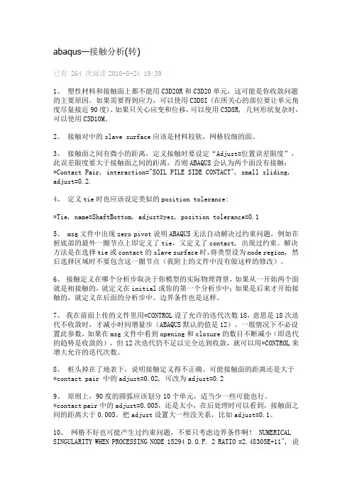
1.1点对面离散与面对面离散【常见问题1-1】在ABAQUS/Standard分析中定义接触时，可以选择点对面离散方法(node-to-surface-dis-cre-tization)和面对面离散方法(surface-to-surface discretization)，二者有何差别?『解答』在点对面离散方法中，从面(slave surface)上的每个节点与该节点在主面(master surface)上的投影点建立接触关系，每个接触条件都包含一个从面节点和它的投影点附近的一组主面节点。

使用点对面离散方法时，从面节点不会穿透(penetrate)主面，但是主面节点可以穿透从面。

面对面离散方法会为整个从面(而不是单个节点)建立接触条件，在接触分析过程中同时考虑主面和从面的形状变化。

可能在某些节点上出现穿透现象，但是穿透的程度不会很严重。

在如图l和图2所示的实例中，比较了两种情况。

1)从面网格比主面网格细：点对面离散(图16-1a)和面对面离散(图16-2a)的分析结果都很好，没有发生穿透，从面和主面都发生了正常的变形。

2)从面网格比主面网格粗：点对面离散(图16-1b)的分析结果很差，主面节点进入了从面，穿透现象很严重，从面和主面的变形都不正常;面对面离散(图16-2b)的分析结果相对较好，尽管有轻微的穿透现象，从面和主面的变形仍比较正常。

从上面的例子可以看出，在为接触面划分网格时需要慎重，无论使用点对面离散还是面对面离散，都应尽量保证从面网格不能比主面网格粗。

关于从面和主面的选择方法，请参见《实例详解》第5.2.2节“定义接触对”。

选用离散方法时，还应考虑以下因素。

1)一般情况下，面对面离散得到的应力和压强的结果精度要高于点对面离散。

2)面对面离散需要分析整个接触面上的接触行为，其计算代价要高于点对面离散。

一般情况下，二者的计算代价相差不是很悬殊，但在以下情况中，面对面离散的计算代价将会大很多：①模型中的大部分区域都涉及到接触问题。

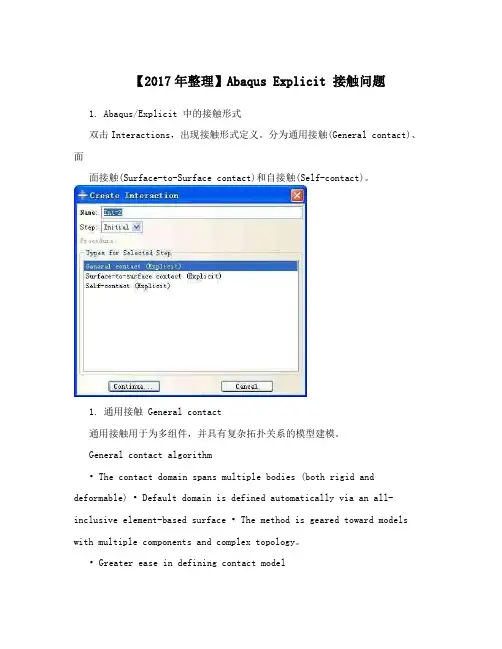
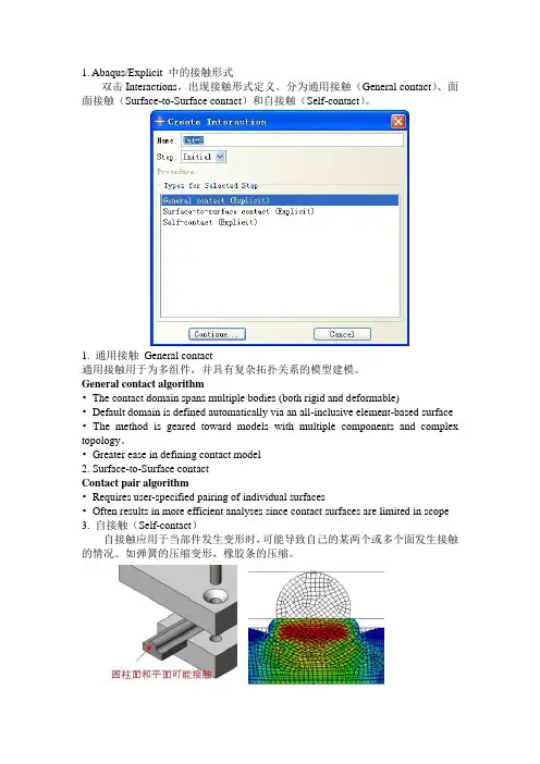
【2017年整理】Abaqus Explicit 接触问题1. Abaqus/Explicit 中的接触形式双击Interactions，出现接触形式定义。

分为通用接触(General contact)、面面接触(Surface-to-Surface contact)和自接触(Self-contact)。

1. 通用接触 General contact通用接触用于为多组件，并具有复杂拓扑关系的模型建模。

General contact algorithm• The contact d omain spans multiple bodies (both rigid and deformable) • Default domain is defined automatically via an all-inclusive element-based surface • The method is geared toward models with multiple components and complex topology。

• Greater ease in defining con tact model2. Surface-to-Surface contactContact pair algorithm• Requires user-specified pairing of individual surfaces• Often results in more efficient analyses since contact surfaces are limited in scope3. 自接触(Self-contact)自接触应用于当部件发生变形时，可能导致自己的某两个或多个面发生接触的情况。

如弹簧的压缩变形，橡胶条的压缩。

• 容易使用• “自动接触”• 节省生成模型的时间• 通用接触算法一般比双面接触算法快机械约束形式• 运动依从 Kinematic contact method (只有接触对形式可用,General contact不可用)默认的运动接触公式达到的计算精度与接触条件相一致。

1. Abaqus/Explicit 中的接触形式双击Interactions，出现接触形式定义。

分为通用接触（General contact）、面面接触（Surface-to-Surface contact）和自接触（Self-contact）。

1. 通用接触General contact通用接触用于为多组件，并具有复杂拓扑关系的模型建模。

General contact algorithm•The contact domain spans multiple bodies (both rigid and deformable)•Default domain is defined automatically via an all-inclusive element-based surface •The method is geared toward models with multiple components and complex topology。

•Greater ease in defining contact model2. Surface-to-Surface contactContact pair algorithm•Requires user-specified pairing of individual surfaces•Often results in more efficient analyses since contact surfaces are limited in scope 3. 自接触（Self-contact）自接触应用于当部件发生变形时，可能导致自己的某两个或多个面发生接触的情况。

如弹簧的压缩变形，橡胶条的压缩。

•容易使用•“自动接触”•节省生成模型的时间•通用接触算法一般比双面接触算法快机械约束形式•运动依从Kinematic contact method（只有接触对形式可用,General contact不可用）默认的运动接触公式达到的计算精度与接触条件相一致。

abaqus接触分析【引】2010-06-03 19:431、塑性材料和接触面上都不能用C3D20R和C3D20单元，这可能是你收敛问题的主要原因。

如果需要得到应力，可以使用C3D8I (在所关心的部位要让单元角度尽量接近90度)，如果只关心应变和位移，可以使用C3D8R, 几何形状复杂时，可以使用C3D10M。

2、接触对中的slave surface应该是材料较软，网格较细的面。

3、接触面之间有微小的距离，定义接触时要设定“Adjust=位置误差限度”，此误差限度要大于接触面之间的距离，否则ABAQUS会认为两个面没有接触：*Contact Pair, interaction="SOIL PILE SIDE CONTACT", small sliding, adjust=0.2.4、定义tie时也应该设定类似的position tolerance:*Tie, name=ShaftBottom, adjust=yes, position tolerance=0.15、 msg文件中出现zero pivot说明ABAQUS无法自动解决过约束问题，例如在桩底部的最外一圈节点上即定义了tie，又定义了contact, 出现过约束。

解决方法是在选择tie或contact的slave surface时，将类型设为node region, 然后选择区域时不要包含这一圈节点（我附上的文件中没有做这样的修改）。

6、接触定义在哪个分析步取决于你模型的实际物理背景，如果从一开始两个面就是相接触的，就定义在initial或你的第一个分析步中；如果是后来才开始接触的，就定义在后面的分析步中。

边界条件也是这样。

7、我在前面上传的文件里用*CONTROL设了允许的迭代次数18，意思是18次迭代不收敛时，才减小时间增量步（ABAQUS默认的值是12）。

一般情况下不必设置此参数，如果在msg文件中看到opening和closure的数目不断减小（即迭代的趋势是收敛的），但12次迭代仍不足以完全达到收敛，就可以用*CONTROL 来增大允许的迭代次数。

abaqus—接触分析(转)已有 264 次阅读2010-8-24 19:39|1、塑性材料和接触面上都不能用C3D20R和C3D20单元，这可能是你收敛问题的主要原因。

如果需要得到应力，可以使用C3D8I (在所关心的部位要让单元角度尽量接近90度)，如果只关心应变和位移，可以使用C3D8R, 几何形状复杂时，可以使用C3D10M。

2、接触对中的slave surface应该是材料较软，网格较细的面。

3、接触面之间有微小的距离，定义接触时要设定“Adjust=位置误差限度”，此误差限度要大于接触面之间的距离，否则ABAQUS会认为两个面没有接触：*Contact Pair, interaction="SOIL PILE SIDE CONTACT", small sliding, adjust=0.2.4、定义tie时也应该设定类似的position tolerance:*Tie, name=ShaftBottom, adjust=yes, position tolerance=0.15、 msg文件中出现zero pivot说明ABAQUS无法自动解决过约束问题，例如在桩底部的最外一圈节点上即定义了tie，又定义了contact, 出现过约束。

解决方法是在选择tie或contact的slave surface时，将类型设为node region, 然后选择区域时不要包含这一圈节点（我附上的文件中没有做这样的修改）。

6、接触定义在哪个分析步取决于你模型的实际物理背景，如果从一开始两个面就是相接触的，就定义在initial或你的第一个分析步中；如果是后来才开始接触的，就定义在后面的分析步中。

边界条件也是这样。

7、我在前面上传的文件里用*CONTROL设了允许的迭代次数18，意思是18次迭代不收敛时，才减小时间增量步（ABAQUS默认的值是12）。

一般情况下不必设置此参数，如果在msg文件中看到opening和closure的数目不断减小（即迭代的趋势是收敛的），但12次迭代仍不足以完全达到收敛，就可以用*CONTROL来增大允许的迭代次数。

Abaqus中的接触问题ABAQUS中一个完整的接触模拟必须包含两部分：一是接触对的定义，其中定义了分析哪些面会发生接触，采用哪种方法判断接触状态，设定主控面和从属面等内容；二是接触面上的本构关系定义。

这里我们通过一个例子简单了解ABAQUS中的接触分析。

（一）接触面的法向模型接触面之间的相互作用包含两个部分：一是接触面的法向作用，二是接触面的切向作用。

ABAQUS对这两部分是分别定义的。

对大部分问题来说，接触面的行为十分明确，即两物体只有在压紧状态时才能传递法向压力P,若两物体之间有间隙时不传递法向压力，这种法向行为在ABAQUS称为硬接触。

这种法向行为在计算中限制了可能发生的穿透现象，但当接触条件从“开”到“闭”时，接触压力会发生剧烈的变化，有时使得接触计算很难收敛。

除了硬接触外，ABAQUS还包含几种软接触，其实质是在闭合时减慢接触压力随过盈量之间的变化速度。

（二）接触面的摩擦模型当接触面处于闭合状态(即有法向接触压力p)时，接触面可以传递切向应力，或称摩擦力。

若摩擦力小于某一极限值时，ABAQUS认为接触面处于粘结状态；若摩擦力大于极限值之后，接触面开始出现相对滑动变形，称为滑移状态。

为了合理地设置摩擦模型。

注意以下几个问题：A极限剪应力：ABAQUS中默认采用Coulomb定律计算极限剪应力：。

在某些情况下，接触压力可能比较大，导致极限剪应力也很大，可能超过能承受的值，此时用户可指定一个所允许的最大剪应力。

B弹性滑移变形：在理想状况下，接触面在滑移状态之前是没有剪切变形的，但这会造成数值计算上的困难，因而ABAQUS引入了一个“弹性滑移变形”的概念，“弹性滑移变形”是指表面粘结在一起时允许发生的少量相对滑移变形。

ABAQUS会根据接触面上单元的长度确定弹性滑移变形(默认为单元典型长度的0.5%，用户也可自己给定)，然后自动选择罚函数计算方法中的刚度。

罚摩擦公式适用于大多数问题，其中包括大部分金属成型问题。

基于ABAQUS/Standard接触问题分析及实例摘要接触问题是许多工程实践中的常见问题，其实际结构系统往往由几个非永久性连接在一起的部分组成。

这些参与接触之间的部分间会有沿接触面法向的相互作用（如接触压力）和沿接触面切向的相互作用（如摩擦作用）。

在有限元分析中，接触条件是一类特殊的不连续约束，它允许力从模型的一部分传递到另一部分。

因为只有当两个表面发生接触时才会有约束产生，当两个面分开时，就不存在约束作用，所以这种约束作用是不连续的。

本文将通过分析ABAQUS/Standard 对接触问题的求解模式，来探讨有限元软件在求解接触问题时的内涵，并通过分析一个冲压金属板的实例来展现更为详尽的过程。

一.ABAQUS/Standard中接触问题在ABAQUS/Standard中，接触问题或是基于表面（surface）或是基于接触单元（contact element）。

因此，首先必须在Interaction模块中各模型上创建可能发生接触的表面并判断哪一对表面可能具有接触约束，即接触对，随后定义控制各接触面之间相互作用的本构模型，这些接触面相互作用的定义包括诸如摩擦行为等。

这里，接触问题属于边界非线性问题，边界条件不再是定解条件，而是待求结果；两接触体间接触面积与压力随外载荷的变化而变，并与接触体的刚性有关。

这是该问题的特点，也是困难所在。

二. 接触面间的相互作用1. 接触面间的法向作用两个接触面分开的距离称为间隙（clearance），当间隙变为零时，表明两个表面形成接触关系（并不意味着接触约束的形成）。

令P为两个接触面之间的接触作用力，当P为零或负值时，接触面分开即接触约束被移开。

当P为正值时，表明接触约束形成（如图1）。

由于接触条件从开（间隙值为正）到闭（间隙值为零）时接触压力可能剧烈变化导致这一过程存在剧烈非线性，因而在Standard 模块中需要更多的增量步迭代以求接触约束变化的过程收敛。

图1 接触约束形成条件2. 常见的接触面间切向作用—摩擦模型当接触表面接触约束形成时，除了法向的接触压力外，还有阻止表面之间相对滑动的切向摩擦力。

1. Abaqus/Explicit 中的接触形式双击Interactions，出现接触形式定义。

分为通用接触（General contact）、面面接触（Surface-to-Surface contact）和自接触（Self-contact）。

1. 通用接触 General contact通用接触用于为多组件，并具有复杂拓扑关系的模型建模。

General contact algorithm•The contact domain spans multiple bodies (both rigid and deformable)•Default domain is defined automatically via an all-inclusive element-based surface• The method is geared toward models with multiple components and complex topology。

• Greater ease in defining contact model2. Surface-to-Surface contactContact pair algorithm• Requires user-specified pairing of individual surfaces• Often results in more efficient analyses since contact surfaces are limited in scope3. 自接触（Self-contact）自接触应用于当部件发生变形时，可能导致自己的某两个或多个面发生接触的情况。

如弹簧的压缩变形，橡胶条的压缩。

•容易使用•“自动接触”•节省生成模型的时间•通用接触算法一般比双面接触算法快机械约束形式•运动依从Kinematic contact method（只有接触对形式可用,General contact不可用）默认的运动接触公式达到的计算精度与接触条件相一致。

1、Defining contact pairs in ABAQUS/StandardAfter the selection of contact pair surfaces, three key factors must be determined when creating a contact formulation:⑴ the contact discretization;⑵ the tracking approach; and⑶the assignment of “master” and “slave” roles to the respective surfaces.1.1the contact discretizationABAQUS/Standard offers two contact discretization options: a traditional “node-to-surface” discretization and a true “surface-to-surface” discretization.1.1.1 Node-to-surface contact discretizationTraditional node-to-surface discretization has the following characteristics:⑴ The slave nodes are constrained not to penetrate into the master surface; however, the nodes of the master surface can, in principle, penetrate into the slave surface⑵ The contact direction is based on the normal of the master surface.⑶ The only information needed for the slave surface is the location and surface area associated with each node; The direction of the slave surface normal and slave surface curvature are not , the slave surface can be defined as a group of nodes —a node-based surface.⑷ Node-to-surface discretization is available even if a node-based surface is not used in the contact pair definitionNode-to-surface contact discretization1.1.2 Surface-to-surface contact discretizationTo optimize stress accuracy, surface-to-surface discretization considers the shape of both the slave and master surfaces in the region of contact constraints.Surface-to-surface discretization has the following key characteristics:⑴ Contact conditions are enforced in an average sense over the slave surface, rather than at discrete points (such as at slave nodes, as in the case of node-to-surface discretization). Therefore, some penetration may be observed at individual nodes; however, large, undetected penetrations of master nodes into the slave surface do not occur with this discretization.⑵ Surface-to-surface discretization is not applicable if a node-based surface is used in the contact pair definition.在某一个迭代步中,面对面的接触计算成本一般较点对面的接触的计算成本高,但多数情况下这个成本不会高很多,只有在下列情况下才会让计算成本急剧增大:⑴模型的绝大部分区域被包含于接触中;⑵当主动面比从属面网格划分还要精细时;⑶ Multiple layers of shells are involved in contact, such that the master surface of one contact pair acts as the slave surface of another contact pair.尽管如此,但点对面的接触需要花费更多的迭代步才能达到数值稳定,从某种意义上来说,在一个分析步中,无法判定到底是用点对面接触还是面对面接触计算成本低.1.2Contact tracking approachesIn ABAQUS/Standard there are two tracking approaches to account for the relative motion of the two surfaces forming a contact pair in mechanical contact simulations:⑴ The finite-sliding tracking approach⑵ The small-sliding tracking approach1.3Fundamental choices affecting the contact formulationYour choice of contact discretization and tracking approach have considerable impact on an analysis. In addition to the qualities already discussed, certain combinations of discretizations and tracking approaches have their own characteristics and limitations associated with them. These characteristics are summarized in Table 1. You should also consider the solution costs associated with the various contact formulationsTable 1 Comparison of contact formulation characteristics选择主动面和从属面的几个原则⑴ Analytical rigid surfaces and rigid-element-based surfaces must always be the master surface.⑵ A node-based surface can act only as a slave surface and always uses node-to-surface contact.⑶ Slave surfaces must always be attached to deformable bodies or deformable bodies defined as rigid.⑷ Both surfaces in a contact pair cannot be rigid surfaces with the exception of deformable surfaces defined as rigid一般来说,当定义两个基于单元的面作为解除对作用面时,当存在一个较小的面和一个较大的面时，一般将较小的面定义为从属面。

Abaqus CAE (ver. 6.9) Contact TutorialProblem DescriptionNote: You do not need to extrude the right vertical edge of the sensor.Analysis Steps1.Start Abaqus and choose to create a new model database2.In the model tree double click on the “Parts” node (or right click on “parts” and select Create)3.In the Create Part dialog box (shown above) name the part anda.Select “3D”b.Select “Deformable”c.Select “Shell”d.Select “Extrusion”e.Set approximate size = 50f.Click “Continue…”4.Create the geometry shown below (not discussed here)a.Click “Done”b.Set Depth = 2c.Click “OK”5.Double click on the “Materials” node in the model tree the new material and give it a descriptionb.Click on the “Mechanical” tabÎElasticityÎElasticc.Define Young’s Modulus and the Poisson’s Ratio (use SI (mm) units)d.Click “OK”6.Double click on the “Sections” node in the model tree the section “ShellProperties” and select “Shell” for the category and “Homogeneous” for thetypeb.Click “Continue…”c.Select the material created above (Steel) and set the thickness to 0.15d.Click “OK”7.Expand the “Parts” node in the model tree, expand the node of the part just created, and double click on“Section Assignments”a.Select the entire geometry, except for the vertical face, in the viewport and press “Done” in theprompt areab.Select the section created above (ShellProperties)c.Specify shell offset if necessaryd.Click “OK”8.Expand the “Assembly” node in the model tree and then double click on “Instances”a.Select “Dependent” for the instance typeb.Click “OK”9.Double click on the “Steps” node in the model tree the step, set the procedure to “General”, select “Static, General”, and click “Continue…”b.Accept the default settings10.Double click on the “BCs” node in the model tree the boundary conditioned “Fixed” and select “Symmetry/Antisymmetry/Encastre” for the typeb.Select the horizontal edges on the vertical surface and click “Done”c.Select “ENCASTRE” for the boundary condition and click “OK”11.Double click on the “BCs” node in the model tree the boundary conditioned “Disp” and select “Displacement/Rotation” for the typeb.Select the top edge of the triangular portion of the geometryc.Set the y‐displacement to ‐312.Double click on the “Interaction Properties” node in the model tree the interaction properties and select “Contact” for the typeb.On the Mechanical tab Select “Tangential Behavior”i.Set the friction formulation to “Frictionless”c.On the Mechanical tab Select “Normal Behavior”i.Because the surfaces do not start in contact, change the constraint enforcement method to“Penalty”13.Double click on the “Interactions” node in the model tree the interaction, select “Surface‐to‐surface contact”, and click continueb.For the master surface select the lower portion of the geometry and click donei.While applying the fixed displacement, the nodes at the tip of the upper portion of thegeometry will make contact at an unknown location on the lower surfaceii.Nodes on the slave surface cannot penetrate the surface formed by the element faces on the master surfacec.Select the color of the surface corresponding to the top surfaced.For the slave surface, set the slave type to “Surface”e.Select the upper portion of the geometry at the free end and click donef.Select the color of the surface corresponding to the bottom surfaceg.Change the contact interaction properties to the one created above (if not already done)14.In the model tree double click on “Mesh” for the Arch part, and in the toolbox area click on the “AssignElement Type” icona.Select the portion of the geometry associated with the boundary conditions and loadb.Select “Standard” for element typec.Select “Linear” for geometric orderd.Select “Shell” for familye.Note that the name of the element (S4R) and its description are given below the element controlsf.Select “OK”15.In the toolbox area click on the “Assign Mesh Controls” icona.Select the portion of the geometry associated with the boundary conditions and loadb.Change the element shape to “Quad”c.Change the technique to “Structured”16.In the toolbox area click on the “Seed Part” icona.Set the approximate global size to 0.2517.In the toolbox area click on the “Mesh Region” iconb.Select the entire geometry, except for the vertical facec.Select “Done”18.In the model tree double click on the “Job” node the job “switch”b.Give the job a description19.In the model tree right click on the job just created and select “Submit”d.Ignore the message about unmeshed portions of the geometrye.While Abaqus is solving the problem right click on the job submitted, and select “Monitor”f.In the Monitor window check that there are no errors or warningsi.If there are errors, investigate the cause(s) before resolvingii.If there are warnings, determine if the warnings are relevant, some warnings can be safely ignored20.In the model tree right click on the submitted and successfully completed job, and select “Results”21.Display the deformed contour of the (Von) Mises stress overlaid with the undeformed geometrya.In the toolbox area click on the following iconsi.“Plot Contours on Deformed Shape”ii.“Allow Multiple Plot States”iii.“Plot Undeformed Shape”22.In the toolbox area click on the “Common Plot Options” icona.Set the Deformation Scale Factor to 1b.Click “OK”23.To change the output being displayed, in the menu bar click on ResultsÎField Outputa.Select the contact pressure at surface nodes (CPRESS)b.Click “OK”。