abaqus拓扑优化例题计算指导
- 格式:pdf
- 大小:1.30 MB
- 文档页数:18
拓扑优化设计的有限元分析使用教程拓扑优化设计是一种优化设计方法,通过对结构的拓扑形状进行优化,以提高结构的性能和效率。
有限元分析是拓扑优化设计中常用的分析方法,能够对结构进行精确的应力和位移分析。
本篇文章将对拓扑优化设计的有限元分析使用进行详细介绍。
第一步:建立有限元模型在进行有限元分析之前,首先需要建立结构的有限元模型。
有限元模型是对实际结构进行离散化的模型,通过对结构进行网格划分,将结构分割成一系列小的单元。
常用的有限元单元包括三角形单元、四边形单元、六面体单元等。
根据实际情况选择适合的有限元单元进行建模。
第二步:定义材料属性和边界条件在建立有限元模型之后,需要为模型定义材料属性和边界条件。
材料属性包括材料的弹性模量、泊松比、密度等。
边界条件包括结构的支撑条件和施加的载荷条件。
根据实际情况为结构定义合适的材料属性和边界条件。
第三步:进行有限元分析有限元分析是对结构进行数值计算的过程,涉及到求解结构的位移和应力。
有限元分析可以通过商业软件实现,例如ABAQUS、ANSYS等。
在进行有限元分析之前,需要选择合适的求解算法和计算参数,并进行设置。
第四步:结果后处理有限元分析完成后,需要对分析结果进行后处理。
后处理包括对位移和应力结果进行可视化和分析。
可以使用后处理软件,如Paraview、Tecplot等,将结果导入进行可视化展示。
通过对结果进行分析,可以评估结构的性能以及进行结构的优化。
第五步:拓扑优化设计在进行有限元分析之后,可以根据分析结果进行拓扑优化设计。
拓扑优化设计的目标是优化结构的形态和拓扑结构,以满足特定的性能要求。
拓扑优化设计方法包括基于密度的方法、基于演化的方法、基于参数化的方法等。
根据实际情况选择适合的拓扑优化设计方法进行优化。
第六步:迭代优化拓扑优化设计是一个迭代的过程,需要进行多次优化迭代来逐步优化结构。
在每次优化迭代中,根据上次的优化结果进行结构的调整和更新,并重新进行有限元分析和后处理。
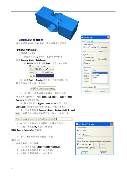
ABAQUS初学者使用算例ABAQUS/CAE实例教程我们将通过ABAQUS/CAE完成上图的建模及分析过程。
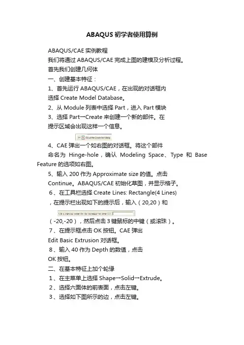
首先我们创建几何体一、创建基本特征:1、首先运行ABAQUS/CAE,在出现的对话框内选择Create Model Database。
2、从Module列表中选择Part,进入Part模块3、选择Part→Create来创建一个新的部件。
在提示区域会出现这样一个信息。
4、CAE弹出一个如右图的对话框。
将这个部件命名为Hinge-hole,确认Modeling Space、Type和Base Feature的选项如右图。
5、输入200作为Approximate size的值。
点击Continue。
ABAQUS/CAE初始化草图,并显示格子。
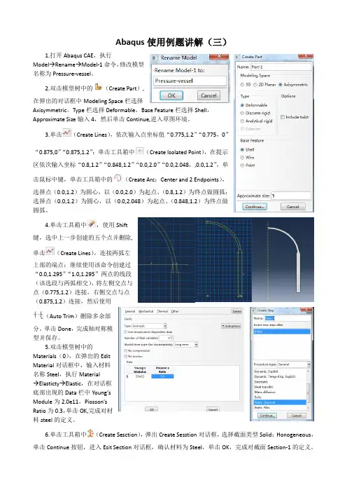
6、在工具栏选择Create Lines: Rectangle(4 Lines),在提示栏出现如下的提示后,输入(20,20)和(-20,-20),然后点击3键鼠标的中键(或滚珠)。
7、在提示框点击OK按钮。
CAE弹出Edit Basic Extrusion对话框。
8、输入40作为Depth的数值,点击OK按钮。
二、在基本特征上加个轮缘1、在主菜单上选择Shape→Solid→Extrude。
2、选择六面体的前表面,点击左键。
3、选择如下图所示的边,点击左键。
4、如右上图那样利用图标创建三条线段。
5、在工具栏中选择Create Arc: Center and 2 Endpoints6、移动鼠标到(40,0.0),圆心,点击左键,然后将鼠标移到(40,20)再次点击鼠标左键,从已画好区域的外面将鼠标移到(40,20),这时你可以看到在这两个点之间出现一个半圆,点击左键完成这个半圆。
7、在工具栏选择Create Circle: Center and Perimeter8、将鼠标移动到(40,0.0)点击左键,然后将鼠标移动到(50,0.0)点击左键。
9、从主菜单选择Add→Dimension→Radial,为刚完成的圆标注尺寸。
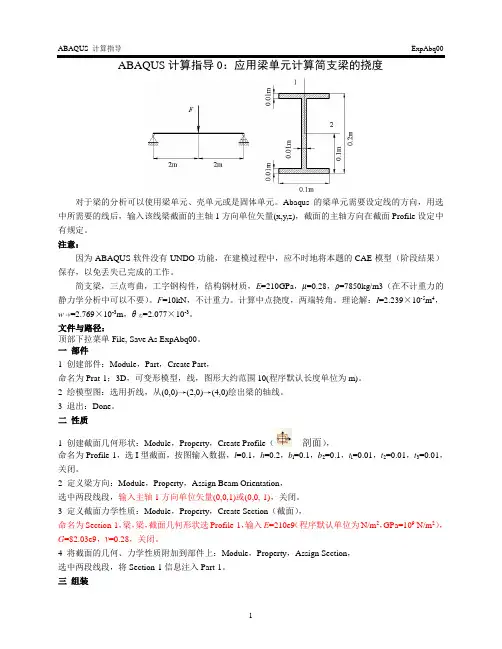
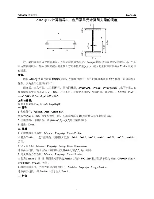
对于梁的分析可以使用梁单元、壳单元或是固体单元。
Abaqus的梁单元需要设定线的方向,用选中所需要的线后,输入该线梁截面的主轴1方向单位矢量(x,y,z),截面的主轴方向在截面Profile设定中有规定。
注意:因为ABAQUS软件没有UNDO功能,在建模过程中,应不时地将本题的CAE模型(阶段结果)保存,以免丢失已完成的工作。
简支梁,三点弯曲,工字钢构件,结构钢材质,E=210GPa,μ=0.28,ρ=7850kg/m3(在不计重力的静力学分析中可以不要)。
F=10kN,不计重力。
计算中点挠度,两端转角。
理论解:I=2.239×10⁻⁵m4,w中=2.769×10⁻³m,θ边=2.077×10⁻³。
文件与路径:顶部下拉菜单File, Save As ExpAbq00。
一部件1 创建部件:Module,Part,Create Part,命名为Prat-1;3D,可变形模型,线,图形大约范围10(程序默认长度单位为m)。
2 绘模型图:选用折线,从(0,0)→(2,0)→(4,0)绘出梁的轴线。
3 退出:Done。
二性质1 创建截面几何形状:Module,Property,Create Profile(剖面),命名为Profile-1,选I型截面,按图输入数据,l=0.1,h=0.2,b l=0.1,b2=0.1,t l=0.01,t2=0.01,t3=0.01,关闭。
2 定义梁方向:Module,Property,Assign Beam Orientation,选中两段线段,输入主轴1方向单位矢量(0,0,1)或(0,0,-1),关闭。
3 定义截面力学性质:Module,Property,Create Section(截面),命名为Section-1,梁,梁,截面几何形状选Profile-1,输入E=210e9(程序默认单位为N/m2,GPa=109 N/m2),G=82.03e9,ν=0.28,关闭。

ABAQUS初学者使用算例ABAQUS/CAE实例教程我们将通过ABAQUS/CAE完成上图的建模及分析过程。
首先我们创建几何体一、创建基本特征:1、首先运行ABAQUS/CAE,在出现的对话框内选择Create Model Database。
2、从Module列表中选择Part,进入Part 模块3、选择Part→Create来创建一个新的部件。
在提示区域会出现这样一个信息。
4、CAE弹出一个如右图的对话框。
将这个部件命名为Hinge-hole,确认Modeling Space、Type和BaseFeature的选项如右图。
5、输入200作为Approximate size的值。
点击Continue。
ABAQUS/CAE初始化草图,并显示格子。
6、在工具栏选择Create Lines: Rectangle(4 Lines),在提示栏出现如下的提示后,输入(20,20)和(-20,-20),然后点击3键鼠标的中键(或滚珠)。
7、在提示框点击OK按钮。
CAE弹出Edit Basic Extrusion对话框。
8、输入40作为Depth的数值,点击OK按钮。
二、在基本特征上加个轮缘1、在主菜单上选择Shape→Solid→Extrude。
2、选择六面体的前表面,点击左键。
3、选择如下图所示的边,点击左键。
4、如右上图那样利用图标创建三条线段。
5、在工具栏中选择Create Arc: Center and 2 Endpoints6、移动鼠标到(40,0.0),圆心,点击左键,然后将鼠标移到(40,20)再次点击鼠标左键,从已画好区域的外面将鼠标移到(40,20),这时你可以看到在这两个点之间出现一个半圆,点击左键完成这个半圆。
7、在工具栏选择Create Circle: Center and Perimeter8、将鼠标移动到(40,0.0)点击左键,然后将鼠标移动到(50,0.0)点击左键。
9、从主菜单选择Add→Dimension→Radial,为刚完成的圆标注尺寸。
ABAQUS/CAE实例教程我们将通过ABAQUS/CAE完成上图的建模及分析过程。
首先我们创建几何体一、创建基本特征:1、首先运行ABAQUS/CAE,在出现的对话框选择Create Model Database。
2、从Module列表中选择Part,进入Part模块3、选择Part→Create来创建一个新的部件。
在提示区域会出现这样一个信息。
4、CAE弹出一个如右图的对话框。
将这个部件命名为Hinge-hole,确认Modeling Space、Type和BaseFeature的选项如右图。
5、输入200作为Approximate size的值。
点击Continue。
ABAQUS/CAE初始化草图,并显示格子。
6、在工具栏选择Create Lines: Rectangle(4 Lines),在提示栏出现如下的提示后,输入(20,20)和(-20,-20),然后点击3键鼠标的中键(或滚珠)。
7、在提示框点击OK按钮。
CAE弹出Edit Basic Extrusion对话框。
8、输入40作为Depth的数值,点击OK按钮。
二、在基本特征上加个轮缘1、在主菜单上选择Shape→Solid→Extrude。
2、选择六面体的前表面,点击左键。
3、选择如下图所示的边,点击左键。
4、如右上图那样利用图标创建三条线段。
5、在工具栏中选择Create Arc: Center and 2 Endpoints6、移动鼠标到(40,0.0),圆心,点击左键,然后将鼠标移到(40,20)再次点击鼠标左键,从已画好区域的外面将鼠标移到(40,20),这时你可以看到在这两个点之间出现一个半圆,点击左键完成这个半圆。
7、在工具栏选择Create Circle: Center and Perimeter8、将鼠标移动到(40,0.0)点击左键,然后将鼠标移动到(50,0.0)点击左键。
9、从主菜单选择Add→Dimension→Radial,为刚完成的圆标注尺寸。
对于梁的分析可以使用梁单元、壳单元或是固体单元。
Abaqus的梁单元需要设定线的方向,用选中所需要的线后,输入该线梁截面的主轴1方向单位矢量(x,y,z),截面的主轴方向在截面Profile设定中有规定。
注意:因为ABAQUS软件没有UNDO功能,在建模过程中,应不时地将本题的CAE模型(阶段结果)保存,以免丢失已完成的工作。
简支梁,三点弯曲,工字钢构件,结构钢材质,E=210GPa,μ=0.28,ρ=7850kg/m3(在不计重力的静力学分析中可以不要)。
F=10kN,不计重力。
计算中点挠度,两端转角。
理论解:I=2.239×10⁻⁵m4,w中=2.769×10⁻³m,θ边=2.077×10⁻³。
文件与路径:顶部下拉菜单File, Save As ExpAbq00。
一部件1 创建部件:Module,Part,Create Part,命名为Prat-1;3D,可变形模型,线,图形大约范围10(程序默认长度单位为m)。
2 绘模型图:选用折线,从(0,0)→(2,0)→(4,0)绘出梁的轴线。
3 退出:Done。
二性质1 创建截面几何形状:Module,Property,Create Profile,命名为Profile-1,选I型截面,按图输入数据,l=0.1,h=0.2,b l=0.1,b2=0.1,t l=0.01,t2=0.01,t3=0.01,关闭。
2 定义梁方向:Module,Property,Assign Beam Orientation,选中两段线段,输入主轴1方向单位矢量(0,0,1)或(0,0,-1),关闭。
3 定义截面力学性质:Module,Property,Create Section,命名为Section-1,梁,梁,截面几何形状选Profile-1,输入E=210e9(程序默认单位为N/m2,GPa=109 N/m2),G=82.03e9,ν=0.28,关闭。
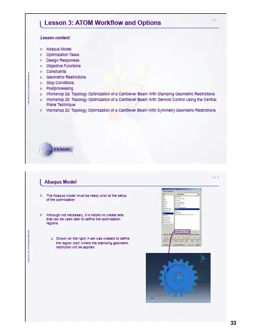
L3.1w w w .3d s .c o m | © D a s s a u l t S y s t èm e sLesson content:Abaqus Model Optimization Tasks Design Responses Objective Functions ConstraintsGeometric Restrictions Stop Conditions PostprocessingWorkshop 2a: Topology Optimization of a Cantilever Beam With Stamping Geometric Restrictions Workshop 2b: Topology Optimization of a Cantilever Beam With Demold Control Using the Central Plane TechniqueWorkshop 2c: Topology Optimization of a Cantilever Beam With Symmetry Geometric RestrictionsLesson 3: ATOM Workflow and Options2.5 hoursL3.2w w w .3d s .c o m | © D a s s a u l t S y s t èm e sAbaqus ModelThe Abaqus model must be ready prior to the setup of the optimizationAlthough not necessary, it is helpful to create sets that can be used later to define the optimization regionsShown on the right: A set was created to define the region (cell) where the stamping geometric restriction will be appliedw w w .3d s .c o m | © D a s s a u l t S y s t èm e sAn optimization task identifies the type of optimization and the design domain for the optimization.The task serves to configure the optimization algorithm to be usedCreate an optimization task from the Model Tree or the Optimization toolbox as shownChoose the type of optimization task accordinglyEach task also contains the design responses, objective functions, constraints, geometric restrictions and stop conditionsIn this lecture we discuss the setup of the task for topology optimizationL3.4w w w .3d s .c o m | © D a s s a u l t S y s t èm e sOptimization Tasks (2/6)For a topology optimization task, the optimization region is selected nextThe elements in the optimization region will constitute the design domainThe whole model is selected by defaultOften, the optimization region will only be a subset of the model.For example, on the right we have removed the deformable shaft from the display so that only the gear is selected as the optimization regionw w w .3d s .c o m | © D a s s a u l t S y s t èm e sHaving chosen the optimization type and region, it is now possible to configure the optimizationThe Basic tab of the optimization task editor allows the user to choose if the load and boundary regions are to be kept frozenFrozen areas are discussed further later in the context of geometric restrictionsL3.6w w w .3d s .c o m | © D a s s a u l t S y s t èm e sOptimization Tasks (4/6)The Density tab allows the user to change thedensity update strategy and configure other related parametersThese settings are only available for the sensitivity-based methodTip: These parameters rarely need to be changed; if necessary, use a more conservative strategy for a more stable optimizationw w w .3d s .c o m | © D a s s a u l t S y s t èm e sThe Advanced tab allows the user to switch to the condition-based approach if desiredThe condition-based approach is usually preferred for stiffness optimizationNote: the sensitivity-based approach is also able to optimize on stiffnessFor the condition-based approach, the user can configure the speed of the update scheme and the volume deleted in the first cycleThe advanced option “Delete soft elements in region” is recommended when solving problems where soft elements may distort excessively and cause convergence difficultyL3.8w w w .3d s .c o m | © D a s s a u l t S y s t èm e sOptimization Tasks (6/6)For sensitivity-based optimization the user may choose between the SIMP and the RAMP material interpolation techniquesRAMP is preferred for problems that are more dynamic in nature because the interpolation scheme is always concave.Criteria for convergence can be set here. Default criteria are usually sufficient.Note: the default penalty factor has been chosen carefully.Values less than 3 shouldn’t be used.Values greater than 3 significantly increase the chance of getting trapped in a local minimaw w w .3d s .c o m | © D a s s a u l t S y s t èm e sDesign responses are output variables that can be used to describe objective functions and constraintsAll available design responses forsensitivity-based optimization are shown on the rightCondition-based optimization can only have strain energy as the objective and volume as the constraintDesign responses can be a summation of values in the region or maximum/minimum of that regionDesign responses can also be summed across steps/load casesL3.10w w w .3d s .c o m | © D a s s a u l t S y s t èm e sDesign Responses (2/3)A design response can be a combination of previously defined design responsesFor example, on the right we have constructed design response D-Response-3 as aweighted combination of D-Response-1 and D-Response-2Sensitivity-based optimization supports the following operators:Weighted combinationDifferenceAbsolute differencew w w .3d s .c o m | © D a s s a u l t S y s t èm e sCondition-based optimization supports many more operators for creating combined termsL3.12w w w .3d s .c o m | © D a s s a u l t S y s t èm e sObjective Functions (1/2)Objective functions can be created from any previously defined design responsesDesign responses can be single term or combined termFurthermore, the objective function is always a weighted sum of the specified design responsesReference values are constants subtracted from the design responseReference values are meaningless for a condition-based topology optimizationL3.13w w w .3d s .c o m | © D a s s a u l t S y s t èm e sObjective Functions (2/2)Three objective target formulations are supported in topology optimizationMINMIN formulation minimizes the weighted sum of the specified design responsesMAXMAX formulation maximizes the sum of the specified design responsesMIN_MAX (minimize the maximum load case)MIN_MAX formulation minimizes the maximum of the two (or more) design responses specified in the objective function editorL3.14w w w .3d s .c o m | © D a s s a u l t S y s t èm e sConstraints (1/2)Constraints are an integral part of a topology optimizationAn unconstrained topology optimization is not allowed.An error is issued for such casesIn a condition-based topology optimization, only volume constraints are allowed and they are enforced as equality constraintsL3.15w w w .3d s .c o m | © D a s s a u l t S y s t èm e sConstraints (2/2)In sensitivity-based optimizations, many more constraints are allowedFilter by constraint while creating the design response to see what output variables can be chosen as constraints (shown below)Combined terms are allowed to be used as constraints (shown bottom right)Constraints are always inequalities in sensitivity-based optimizationL3.16w w w .3d s .c o m | © D a s s a u l t S y s t èm e sGeometric Restrictions (1/7)Geometric restrictions are additional constraints which are enforced independent of the optimizationGeometric restrictions can be used to enforce symmetries or minimum member sizes that are desired in the final designDemold control is perhaps the most important geometric restriction.It enables the user to place constraints such that the final design can be manufactured by casting.w w w .3d s .c o m | © D a s s a u l t S y s t èm e sFrozen areaFrozen area constraints ensure that no material is removed from the regions designated as frozen (relative density here is always 1)These constraints are particularly important in regions where loads and boundary conditions are specified since we don’t want these regions to become voids.In the gear example, the gear teeth and the inner circumference were kept frozen.Prevents losing contact with the shaft or losing the load path.FrozenL3.18w w w .3d s .c o m | © D a s s a u l t S y s t èm e sGeometric Restrictions (3/7)Member sizeTopology optimization can sometimes lead to thin or thick members that can be problematic to manufactureMember size restrictions provide filters to control the size of the membersUsers input a filter diameterNote:Maximum thickness restriction (and therefore enveloperestriction) is available only in sensitivity-based optimizationThe exact member size specified by the filter diameter isn’t guaranteedw w w .3d s .c o m | © D a s s a u l t S y s t èm e sDemold controlIf the topology obtained from the optimization is to be produced by casting, the formation of cavities and undercuts needs to be prevented by using demold controlDemold region: region where the demold control restriction is activeCollision check region: region where the removal of an element results in a hole or an undercut is checkedI.This region is same as the demold region by defaultII.This region should always contain at least the demold regionThe pull direction: the direction in which the two halves of the mold would be pulled in (as shown, bottom right)Center plane: central plane of the mold (as shown, bottom right)I.Can be specified or calculated automaticallyL3.20w w w .3d s .c o m | © D a s s a u l t S y s t èm e sGeometric Restrictions (5/7)Demold control (cont’d)The stamping option enforces the condition that if one element is removed from the structure, all others in the ± pull direction are also removedIn the gear example, a stamping constraint was used to ensure that only through holes are formed.Forging is a special case of casting. The forging die needs to be pulled in only one direction.The forging option creates a fictitious central plane internally on the back plane (shown below) so that pulling takes place in only one directionL3.21w w w .3d s .c o m | © D a s s a u l t S y s t èm e sGeometric Restrictions (6/7)SymmetryTopology optimization of symmetric loaded components usually leads to a symmetric designIn case we want a symmetric design but the loading isn’t symmetric, it is necessary to enforce symmetryPlane symmetryRotational symmetryCyclic symmetryPoint symmetryL3.22w w w .3d s .c o m | © D a s s a u l t S y s t èm e sGeometric Restrictions (7/7)It is possible to overconstrain the optimization.Care must be taken when specifying combinations of geometric restrictions.Examples:Planar symmetry can be combined with a pull direction if the pull direction is perpendicular or parallel to the symmetry plane.Rotation symmetry and the definition of a pull direction: this combination is possible if the pull direction is parallel to the axis of rotation.Two reflection symmetries can be combined if the planes are perpendicular.In general, begin the optimization study without geometric restrictions. Add them into the model one by one.L3.23w w w .3d s .c o m | © D a s s a u l t S y s t èm e sStop ConditionsThe optimization may be stopped before convergence is achieved if the stop conditions are achievedStop conditions can be constructed on displacements and stressesStop conditions are only supported in shape optimizationL3.24w w w .3d s .c o m | © D a s s a u l t S y s t èm e sPostprocessing (1/10)The relative densities of the elements in the optimization region are available in the field output variable MAT_PROP_NORMALIZEDw w w .3d s .c o m | © D a s s a u l t S y s t èm e sIn order to access the field output showing the relative densities of elements, switch to the step named ATOM OPTIMIZATIONFrom the main menu bar, select Results →Step/FrameSelect ATOM OPTIMIZATION as the step to visualizePlot contours of MAT_PROP_NORMALIZEDNote: Only the undeformed shape will be plotted. If the deformed shape is desired, switch back to Step-1_Optimization (or as named in your model)L3.26w w w .3d s .c o m | © D a s s a u l t S y s t èm e sPostprocessing (3/10)IsosurfacesThe soft elements can be visualized as voids using the Opt_surface cut in the View Cut ManagerRelative densities of the elements are centroidal quantities that are extrapolated and averaged at the nodes in order to obtain field outputAn isosurface is created that separates the soft elements from the hard elementsw w w .3d s .c o m | © D a s s a u l t S y s t èm e sWhat went wrong here?Can we tell by looking at stress or displacement plots?Iso value = 0.9 Iso value = 0.3L3.28w w w .3d s .c o m | © D a s s a u l t S y s t èm e sPostprocessing (5/10)Iso value = 0.9 Iso value = 0.3Note: Always plot MAT_PROP_NORMALIZED as field output and ensure that the isosurface is not cutting through fully dense elementsw w w .3d s .c o m | © D a s s a u l t S y s t èm e sBelow, isosurfaces are generated on element output (MAT_PROP_NORMALIZED) that is averaged at nodes with the averaging threshold at 100%Iso value = 0.9Iso value = 0.3L3.30w w w .3d s .c o m | © D a s s a u l t S y s t èm e sPostprocessing (7/10)ExtractionExtraction is a process of obtaining a surface mesh (STL format or its equivalent in an Abaqus input file) from a topology optimization resultOnce the isosurface is identified, new interior edges and surfaces are identified.Nodes are created on interior faces and a triangular mesh is created on the portion of the model to be retained.SmoothingThe isosurface provides first-order smoothing of a topology optimization resultDuring extraction the nodes on the interior surfaces are moved to achieve additional smoothing of the isosurfacew w w .3d s .c o m | © D a s s a u l t S y s t èm e sExtraction (cont’d)Reduction is the process of reducing the number of triangles in the STL representationThis is useful when converting a large STL file to a SAT file which can be imported and meshed in Abaqus for further analysisNote: you will need to use other DS tools such as SOLIDWORKS or CATIA for this conversionL3.32w w w .3d s .c o m | © D a s s a u l t S y s t èm e sPostprocessing (9/10)Optimization reportEnsure that the optimization constraints have been satisfied within toleranceOptimization_report.csv is created in the working directoryITERATION OBJECTIVE-1 OBJ_FUNC_DRESP:COMPLIANCE OBJ_FUNC_TERM:COMPLIANCE OPT-CONSTRAINT-1:EQ:VOL Norm-Values: 0.6456477 0.6456477 0.6456477 0.8000001 0 0.6456477 0.6456477 0.6456477 1 1 0.6497207 0.6497207 0.6497207 0.948712 2 0.6501995 0.6501995 0.6501995 0.9437472 3 0.6512569 0.6512569 0.6512569 0.93827784 0.6520502 0.6520502 0.6520502 0.9331822 0.6916615 0.6916615 0.6916615 0.831561823 0.6954725 0.6954725 0.6954725 0.8268944 24 0.7028578 0.7028578 0.7028578 0.8217635 25 0.8512989 0.8512989 0.8512989 0.8169149 26 0.7232164 0.7232164 0.7232164 0.8110763 27 0.7404507 0.7404507 0.7404507 0.8057563 28 0.7356095 0.7356095 0.7356095 0.8024307w w w .3d s .c o m | © D a s s a u l t S y s t èm e sHistory outputOptimization_report.csv should not be accessed while the optimization is running.Use the history output variables in Abaqus/CAE to monitor constraints and objectivesL3.34w w w .3d s .c o m | © D a s s a u l t S y s t èm e s1.In this workshop you will:a.become familiar with setting up, submitting and postprocessing a topology optimization problem with astamping geometric restrictionWorkshop 2a: Topology Optimization of a Cantilever Beam With Stamping Geometric RestrictionsL3.35w w w .3d s .c o m | © D a s s a u l t S y s t èm e s1.In this workshop you will:a.further explore demold control geometric restrictions, specifically with the central plane technique whichensures that the final design proposal is moldableWorkshop 2b: Topology Optimization of a Cantilever Beam With Demold Control Using the Central Plane Technique30 minutesL3.36w w w .3d s .c o m | © D a s s a u l t S y s t èm e s1.In this workshop you will:a.explore various symmetry restrictions available in the topology optimization modulee symmetry restrictions to create specific patterns in the design area as required for ease ofmanufacturing a particular componentWorkshop 2c: Topology Optimization of a Cantilever Beam With Symmetry Geometric Restrictions。

Abaqus中Topology和Shape优化指南目录1. 优化模块界面......................................................................................................- 1 -2. 专业术语..............................................................................................................- 1 -3.定义拓扑优化Task(general optimization和condition-based optimization).......- 2 -3.1 General Optimization 参数设置.................................................................- 3 -3.1.1 Basic选项参数..................................................................................- 3 -3.1.2 Density选项参数..............................................................................- 4 -3.1.3 Perturbation选项参数.......................................................................- 5 -3.1.4 Advanced选项参数...........................................................................- 5 -3.2 Condition-based topology Optimization 参数设置....................................- 6 -3.2.1 Basic选项参数..................................................................................- 7 -3.2.2 Advanced选项参数...........................................................................- 7 -4 定义Shape Optimization Task方法....................................................................- 8 -4.1 Basic选项参数............................................................................................- 8 -4.2 Mesh Smoothing Quality选项参数............................................................- 9 -4.3 Mesh Smoothing Quality选项参数..........................................................- 11 -5 定义design response变量方法.........................................................................- 13 -5.1 单个design response定义方法...............................................................- 14 -5.2 combined design response定义方法........................................................- 15 -5.3 design response使用注意事项.................................................................- 17 -5.3.1 定义design response的操作.........................................................- 17 -5.3.2 condition-based topology optimization的design response............- 18 -5.3.3 general topology optimization的design response..........................- 18 -5.3.4 design response for shape optimization...........................................- 21 -6 定义objective function方法..............................................................................- 22 -6.1 目标函数定义...........................................................................................- 23 -6.2 目标函数的运算.......................................................................................- 23 -6.2.1 min运算..........................................................................................- 23 -6.2.2 max运算..........................................................................................- 24 -6.2.3 minimizing the maximum design response......................................- 24 -7 定义Constraints方法........................................................................................- 24 -8 定义Geometric restrictions方法.......................................................................- 25 -8.1 Defining a frozen area................................................................................- 26 -8.2 Specifying minimum and maximum member size....................................- 26 -8.3 maintaining a moldable structure(可拔模结构)........................................- 27 -8.4 maintaining a stampable structure(冲压成型结构)...................................- 28 -8.5 Specifying a symmetric structure...............................................................- 29 -8.6 Applying additional restrictions during a shape optimization...................- 31 -8.7 Combining geometric constraints..............................................................- 31 -9 定义Stop conditions方法..................................................................................- 32 -9.1 Global stop conditions...............................................................................- 32 -9.2 Local stop conditions.................................................................................- 33 -10 Abaqus优化模块支持.......................................................................................- 34 -10.1 Support for analysis types........................................................................- 34 -10.2 Support for geometric nonlinearities.......................................................- 34 -10.3 Support for multiple load cases................................................................- 34 -10.4 Support for acceleration loading..............................................................- 35 -10.5 Support for contact during the optimization............................................- 35 -10.6 Restrictions on an Abaqus model used for topology optimization..........- 35 -10.7 Restrictions on an Abaqus model used for shape optimization...............- 35 -10.8 Support materials in the design area........................................................- 36 -10.8.1 Materials supported by condition-based topology optimization....- 36 -10.8.2 Materials supported by general topology optimization.................- 36 -10.8.3 Material support in shape optimization..........................................- 37 -10.9 支持的单元类型.....................................................................................- 37 -10.9.1 支持的二维实体单元...................................................................- 37 -10.9.2 支持的三维实体单元...................................................................- 38 -10.9.3 支持的对称实体单元...................................................................- 39 -10.9.4 额外支持的单元...........................................................................- 39 -11. Job模块中优化过程的设置............................................................................- 40 -11.1 优化过程的理解.....................................................................................- 40 -11.2 Optimization Process Manager................................................................- 42 -12 拓扑优化理论...................................................................................................- 42 -12.1 General Topology Optimization理论......................................................- 43 -12.1.1 SIMP(Solid Isotropic Material With Penalization Method).......- 43 -12.1.2 RAMP(Rational Approximation of Material Properties)...............- 43 -12.1.3 Gradient-based methods.................................................................- 43 -12.2 General与Condition-based Topology Optimization对比.....................- 44 -13 拓扑优化结果后处理.......................................................................................- 44 -13.1 单元相对密度值.....................................................................................- 44 -13.2 Isosurfaces................................................................................................- 45 -13.3 Extraction.................................................................................................- 47 -14 形貌优化后处理...............................................................................................- 48 -14.1 向量DISP_OPT.....................................................................................- 48 -14.2 场变量DISP_OPT_V AL........................................................................- 48 -14.3 正常分析步中的优化迭代过程中的应力和位移等场变量.................- 49 -14.4 Extracting a surface mesh........................................................................- 49 -15 几何非线性的开与闭对拓扑优化结果的影响...............................................- 50 -16. 形貌优化中的几何约束..................................................................................- 53 -16.1 Demold control(脱模控制)......................................................................- 53 -16.2 Turn control(车床加工控制)...................................................................- 55 -16.3 Drill control(钻孔控制)...........................................................................- 56 -16.4 Planar symmetry(平面对称约束)............................................................- 57 -16.5 Stamp control(锻造控制)........................................................................- 58 -16.6 Growth约束............................................................................................- 58 -16.7 Design direction约束..............................................................................- 59 -16.8 Penetration check(穿越检查)..................................................................- 60 -1. 优化模块界面2. 专业术语① optimization task:对优化任务的一个定义,即定义一个优化Job;② design responses:一个设计响应可以直接从输出数据库中提取,例如模型的体积,另外,对于拓扑优化模块的设计响应不仅可以直接从输出数据库中提取,而且可以计算设计响应,如模型的应变能;③ objective function:目标函数指的是设计响应的函数值或者是一组设计响应的组合,如整个模型的应变能的最小值;④ constraints:约束是一个设计响应的函数值,但不能是多个设计响应组合的函数值;⑤ geometric restriction:A geometric restriction places restrictions on the changes that the Abaqus Topology Optimization Module can make to the topology of the model. Geometrical restrictions include frozen regions from which material cannot be removed and manufacturing constraints, such as restrictions on cavities and undercuts, that would prevent the optimized model from being removed from a mold⑥ stop condition:停止条件是对优化计算收敛的一个指示器,如当在一个指定数量的迭代后一个优化被认为完成了;global stop condition定义了优化迭代的最大数目,local stop condition指定了优化迭代达到所需最小或最大数目;⑦ optimization processes:需要在job模块中创建;⑧ design varible:对于topo优化,优化区域的每个单元的密度即为设计变量;而shape优化,优化区域表面单元的节点的位移即为设计变量;⑨ design cycle:优化过程中的每个迭代成为design cycle;【提示】:I、优化算法总是在满足了约束的基础上才开始最大或最小化目标函数;II、一个优化任务中最多只能包含一个体积约束;【附英文原版】3.定义拓扑优化Task(general optimization和condition-based optimization)3.1 General Optimization 参数设置 3.1.1 Basic选项参数3.1.2 Density选项参数3.1.3 Perturbation选项参数3.1.4 Advanced选项参数在优化计算过程中,拓扑优化模块会自动给优化区域分配一个指定的质量来满足约束和目标函数,在优化结束时,整个优化区域的结构包含了硬单元(hard elements)和软单元(soft elements),其中软单元对结构的刚度没有任何影响,但是影响着结构的自由度,因此会影响优化计算的速度。
Workshop 3Shape Optimization of a Plate with a Hole© Dassault Systèmes, 2012Topology and Shape Optimization in AbaqusIntroductionIn this workshop you will become familiar with the process of setting up, submitting, monitoring and postprocessing a shape optimization problem using Abaqus/CAE.A finite element model of a plate with a hole is provided (see Figure W3–1). You will import this model into Abaqus/CAE and then perform a shape optimization on it.Preliminaries1. Enter the working directory for this workshop:../atom/plate2. Start a new session of Abaqus/CAE using the following command:abaqus caewhere abaqus is the command used to run Abaqus.3. In the Start Session dialog box, underneath Create Model Database , click With Standard/Explicit Model .4. From the main menu bar, select File →Run Script .5. In the Run Script dialog box, select ws_atom_plate.py and click OK .6. A model named hole-plate-quarter will be created.Figure W3– 1 Quarter symmetry model of a plate with a hole.171Examining the finite element modelIn this finite element model we are interested in the static response of a plate with a hole tomultiple load cases. Taking advantage of symmetry, we construct only a quarter symmetrymodel. The model consists of the following:1.Parts: The model consists of a single part named PART–1.2.Mesh: The plate is meshed with CPS4 elements.3.Materials: Material properties of steel have been assigned to the plate.4.Steps: Two steps, one for each load case are specified. Nonlinear geometric effects areconsidered.5.Loads: Two loads of magnitude 200 and 100 are specified in the X- and Y-directions, inSteps 1 and 2, respectively. The loads are not propagated from one step to another; thus,they represent independent load cases.6.Boundary conditions: Symmetry boundary conditions are applied to appropriate edges.Before proceeding with the optimization analysis, examine the finite element model.To examine the finite element model:1. In the Model Tree, click to expand the model hole–plate–quarter as shown in FigureW3–2.2.Expand the following containers: Parts, Materials, Assembly, Steps, Loads and BCs.3.Right-click on each of the items in the containers and choose Edit from the menu thatappears.4.Click Cancel in order to avoid making changes to the analysis.Figure W3–2 Model Tree for quarter plate model.© Dassault Systèmes, 2012 Topology and Shape Optimization in Abaqus 172© Dassault Systèmes, 2012 Topology and Shape Optimization in AbaqusCreating and submitting an analysis job Once you have examined the model, you will submit an analysis job to ensure that the model runs without error and produces meaningful results.To create and submit an analysis job:1. Switch to the Job module.2. From the main menu bar, select Job →Manager .3. From the buttons on the bottom of the Job Manager , click Create to create a job.4. In the Create Job dialog box that appears:a. Name the job hole –plate –quarter and select the model hole –plate –quarteras the source; click Continue .5. In the Edit Job dialog box that appears, click OK to accept all defaults.6. From the buttons on the right side of the Job Manager , click Submit to submit your job for analysis. The status field will show Running . When the job completes successfully, the Status field will change to Completed as shown in Figure W3–3.Figure W3–3 Job Manager.7. In the Job Manager , click Results to postprocess the analysis results.8. In the Visualization toolbox, plot the Mises stress distribution for each of the load cases as shown in Figure W3–4.Figure W3–4 Contour plots of Mises stress.9. Return to the Job module and dismiss the Job Manager.173Defining a shape optimizationIn shape optimization, typically the goal is to homogenize the stress on the surface of acomponent by adjusting the surface nodes. Thus, the minimization is achieved byhomogenization. Shape optimization is not limited to minimizing stresses; it may be extended to plastic strains, natural frequencies, etc.In this workshop you will homogenize the Mises stress on the periphery of a hole in a plate. You will consider two load cases simultaneously, ensuring that the plate is equally stressed in bothload cases and therefore equally likely to fail (or survive) either load case.The workflow for shape optimization is exactly the same as that for topology optimization.Creating an optimization task:1.Switch to the Optimization module (Figure W3–5).Figure W3–5 Switching to the Optimization module.2.From the main menu bar, select Task→Create.3.In the Create Optimization Task dialog box that appears: the optimization task optimize-shape.b.Select Shape optimization as the type and click Continue.c.You will be prompted to select an optimization region.d.Select the set DESIGN_NODES, as shown in Figure W3–6.© Dassault Systèmes, 2012 Topology and Shape Optimization in Abaqus 174Figure W3–6 Selecting the optimization region.In shape optimization the design variables are the positions of the surface nodes; thus, the optimization region is always a set of nodes.Next, you will select and configure the optimization algorithm.In the Edit Optimization Task dialog box (Figure W3–7):1.In the Basic tabbed page, select Freeze boundary condition regions.2.Select Specify smoothing region, and select the whole model.3.Select Fix all as the Number of node layers adjoining the task region to remain free.4.In the Mesh Smoothing Quality tabbed page, set the Target mesh quality to Medium.5.Accept all defaults in the Advanced tabbed page.6.Click OK.© Dassault Systèmes, 2012 Topology and Shape Optimization in Abaqus175© Dassault Systèmes, 2012 Topology and Shape Optimization in AbaqusFigure W3–7 Optimization task editor.You have now configured the shape optimization algorithm. Next, you will define design responses.Creating design responses:1. From the main menu bar, select Design Response →Create .2. In the Create Design Response dialog box that appears:a. Name the design response Mises –Stress –step1.b. Accept Single-term as the type, and click Continue .c. You will be prompted to select the design response region type.d. In the prompt area, select Whole Model as the design response region.3. In the Edit Design Response dialog box that appears (Figure W3–8):a. In the Variable tabbed page, select Stress and Mises hypothesis .b. Note that the field Operator on values in region is set to Maximum value bydefault.c. Switch to the Steps tabbed page, select Specify and click to add a step.d. Select Step-1 from the Step and Load Case drop-down list.e. Click OKto create the design response.176© Dassault Systèmes, 2012 Topology and Shape Optimization in AbaqusFigure W3–8 Design response for the strain energy.4. Similarly, define a design response for Step –2.a. Name the design response Mises –Stress –step2.5. Similarly, define a design response for the volume (see Figure W3–9).a. Name the design response Volume .Figure W3–9 Design response for the volume.177© Dassault Systèmes, 2012 Topology and Shape Optimization in AbaqusNext, you will create an objective function. Creating an objective function:1. From the main menu bar, select Objective Function→Create .2. In the Create Objective Function dialog box that appears:a. Name the objective function optimize-shape and click Continue .3. In the Edit Objective Function dialog box that appears (Figure W3–10):a. Click to add all design responses eligible to participate in an objectivefunction.b. Leave the Reference Target field at the Default setting.c. Change the Target to Minimize the maximum design response values .d. Click OK .Figure W3–10 Objective function optimize-shape .Next, you will create a volume constraint.The purpose of creating volume constraints in a shape optimization is to ensure that the overall volume of the component remains the same. In most cases it is undesirable to simply addmaterial to reduce stress. Rather, material is redistributed to minimize stress. Volume constraints ensure that either no material is added or very little material is added as a result of the shape optimization.Creating a constraint:1. From the main menu bar, select Constraint →Creat e .2. In the Create Constraint dialog box that appears:a. Name the constraint volume-constraint and click Continue .3. In the Edit Optimization Constraint dialog that appears (Figure W3–11):a. Click the drop-down menu for the Design Response , and select Volume .b. Toggle on A fraction of the initial value and enter 1.c. Click OKto create the optimization constraint for volume.178Figure W3–11 Optimization constraint on volume.The setup of the optimization task is now complete. Next, you will create and submit an optimization process.Creating an optimization process:1.Switch to the Job module.2.From the main menu bar, select Optimization→Create.3.In the Edit Optimization Process dialog box that appears (Figure W3–12): the optimization process optimize-shape.b.In the Description field of the dialog box, enter shape optimization.c.Note the Maximum cycles field is set to 10 by default for shape optimization.d.Click OK.Figure W3–12 Edit optimization process.© Dassault Systèmes, 2012 Topology and Shape Optimization in Abaqus179Submitting an optimization process:1.From the main menu bar, select Optimization→Manager.2.From the buttons on the right side of the Optimization Process Manager, click Validateto validate the optimization process.a.When the validation process completes successfully, the Status field will changeto Check Completed.3.Click Submit in the Optimization Process Manager.4.Once the Status changes to Running,click Monitor if you wish to monitor the progressof the optimization process.Postprocessing shape optimization resultsYou may postprocess the solution when the optimization process is complete.Opening the Abaqus output database file:1.Click Results in the Optimization Process Manager.Note that the Abaqus output database file is stored in the folder named ATOM_POST. Allsolution folders generated by ATOM have the structure shown in Figure W3–13.The .odb file stored in the folder ATOM_POST contains the optimization results. Note thatthe history data available for optimization are also available inoptimization_report.csv. You may access this file after the optimization is completebut not during it. Abaqus will stop writing to the file if it is opened during the run. Thefolders SAVE.dat, SAVE.inp, etc. are archives of the Abaqus runs that were performed bythe optimizer. The file atom.out contains the output log from the optimizer.Figure W3–13 File structure from an optimization run.© Dassault Systèmes, 2012 Topology and Shape Optimization in Abaqus 180Contour plotting the shape change:1.From the main menu bar, select Result→Step/Frame.a.From the Step/Frame dialog box, select the ATOM OPTIMIZATION step.b.Select Frame10 (or the highest iteration available to you) from the list ofavailable frames.c.Click OK to close the Step/Frame dialog box.d.In the Visualization toolbox, click and set the Deformation Scale Factor to1.e.In the Field Output toolbar:i. Set the Primary variable to DISP_OPT _VAL.ii.Set the Deformed variable to DISP_OPT.f.In the Visualization toolbox, click and hold .g.Select the last icon to plot contours on both the deformed and undeformedshapes.The contour plot of the deformed shape overlaid on the undeformed shape after 10iterations appears as shown in Figure W3–14. The figure shows the displacementsapplied by the optimizer (shape change) as a scalar. Growth is visualized in red whileshrinkage is visualized in blue. This plot provides an understanding of where themodel is shrinking and where it is growing. Recall that the volume was constrained toremain constant; thus, the growth and shrinkage balance each other. The plot alsoshows that the mesh in the interior moves as a result of the smoothing that wasapplied.Figure W3–14 Contour plot of DISP_OPT_VAL at 10 cycles.© Dassault Systèmes, 2012 Topology and Shape Optimization in Abaqus181Figure W3–15 shows the results after 150 iterations. As seen in the two figures, the difference in the peak values of DISP_OPT_VAL between the two jobs is not large. This implies that theshape optimization only made minor corrections to the shape between iterations 10 and 150.Figure W3–15 Contour plot of DISP_OPT_VAL at 150 cycles.While creating the objective function we had chosen to minimize the maximum design response values. The formulation finds the maximum objective function term and seeks to minimize itduring each design iteration. Given that the optimizer employs a large number of iterations, it is expected that the objective function terms will be more or less equal in magnitude at end of theoptimization. In this example, the stress due to the load in steps 1 and 2 is more or less equalafter the shape optimization. Thus, the plate is not more likely to fail in one load case versus the other.© Dassault Systèmes, 2012 Topology and Shape Optimization in Abaqus 182Plot the Mises stress and compare the peak stress from each of the load cases.Plotting the Mises stress:1.From the main menu bar, select Result→Step/Frame.a.From the Step/Frame dialog box, select step Step-1_Optimization.b.Select Frame10 from the list of available frames.c.Click OK to close the Step/Frame dialog box.d.In the Visualization toolbox, click and set the Deformation Scale Factor to300.e.In the Field Output toolbar:i. Set the Primary variable to S (Int Pt) and select Mises as the component.ii.Set the Deformed variable to U.f.In the Visualization toolbox, click to plot contours on both the deformed andundeformed shapes.g.Repeat steps a-f for Step-2_Optimization.The results are shown in Figure W3–16 (a and b). Note the significant differencebetween the peak values of Mises stress after 10 iterations. This is a strong indicationthat the MIN_MAX formulation needs more iterations to achieve its goal.Figure W3–16 (c and d) shows the results from a solution that was allowed to run for150 iterations. The difference in the peak stresses is now significantly reduced.© Dassault Systèmes, 2012 Topology and Shape Optimization in Abaqus183a.Mises stress Step-1 at 10 cycles.b. Mises stress Step-2 at 10 cycles.c.Mises stress Step-1 at 150 cycles.d. Mises stress Step-2 at 150 cycles.Figure W3–16 Contour plots of Mises stress.© Dassault Systèmes, 2012 Topology and Shape Optimization in Abaqus 184Plot the history output for variables OBJ_FUNCTION_DRESP: MISES-STRESS-STEP1 andOBJ_FUNCTION_DRESP:MISES-STRESS-STEP2. Compare the magnitudes, as shown inFigure W3–17.To plot history output:1.From the main menu bar, select Result→History Output.2.From the History Output dialog box that appears, select the ATOM OptimizationHistory variables.3.Click Plot to plot the selected variables.4.Click Dismiss to dismiss the dialog box.The red arrow in Figure W3–17 indicates the results obtained in 10 iterations. Clearly 10iterations were not sufficient for the optimization process to converge.Figure W3–17 History plots.© Dassault Systèmes, 2012 Topology and Shape Optimization in Abaqus185Finally, it is important to clarify that the MIN_MAX formulation may result in the increase insome objective function terms as it operates on others, even though a minimization wasspecified. In Figure W3–17 we see that during the first 60 iterations the peak Mises stress forStep-1 reduces while the peak Mises stress for Step-2 increases. The increase in peak Misesstress for Step-2 is nothing more than an unavoidable side effect of the shape change that wasdriven by Step-1 (the Mises stress in Step-1 was greater during the first 60 iterations). Atapproximately the 60th iteration, Step-2 begins to dominate the shape change and the Mises stress for Step-2 begins to reduce. Fortunately, the subsequent shape changes do not adversely affectthe Mises stress in Step-1.Note: A script that creates the model described in these instructions is availablefor your convenience. Run this script if you encounter difficulties following theinstructions outlined here or if you wish to check your work. The script is named ws_atom_plate_answer.pyand is available using the Abaqus fetch utility.© Dassault Systèmes, 2012 Topology and Shape Optimization in Abaqus 186。