matlab瑞利衰落信道仿真
- 格式:docx
- 大小:472.71 KB
- 文档页数:5
摘要:本文基于MATLAB对移动衰落信道进行仿真。
重点利用JAKES法对瑞利信道进行了确定性模型仿真,对其功率谱密度和自相关函数进行了讨论。
通过比较仿真模型与参考模型,说明了仿真模型的正确性。
同时,仿真结果表明,仿真结果的特性主要取决于最大多普勒频移与谐波个数这两个参数。
关键词:瑞利信道;功率谱密度;自相关函数;JAKES法;最大多普勒频移Mobile Fading Channel Simulation Based on MATLABAbstract:In this thesis, mobile fading channel is simulated based on MATLAB. It mainly focuses on the deterministic model simulation of Rayleigh channel using JAKES method, and its power spectral density and autocorrelation function are discussed. By comparing the simulation model with the reference model, it demonstrates the correctness of simulation models. At the same time, the simulation results indicate that the results are mainly depending on following two parameters: the maximum Doppler frequency shifts and the number of harmonic waves.Keywords: Rayleigh channel;power spectral density;autocorrelation function;Jakes method;maximum Doppler shift目录前言 (1)第一章绪论 (2)1.1 研究背景及意义 (2)1.2 研究内容 (2)第二章无线信道的概念与特性 (3)2.1 移动无线信道的概念 (3)2.2 移动无线信道基本理论 (3)2.3 移动无线信道的类型 (4)2.3.1 传播路径损耗模型 (4)2.3.2 大尺度传播模型 (4)2.3.3 小尺度传播模型 (4)2.4 移动无线信道的衰落 (5)2.5 瑞利衰落信道模型的实现 (5)第三章确定性信道过程的理论导论 (8)3.1 确定性信道建模的原理 (8)3.1.1成形波器法 (8)3.2.2正弦波叠加法 (9)3.2 确定性过程的基本性质 (11)第四章确定性过程模型参数的计算方法 (12)4.1 离散多普勒频率和多普勒系数的计算方法 (12)4.2 多普勒相位的计算方法 (15)4.3 确定性瑞利过程的衰落时间间隔 (16)第五章JAKES功率谱密度与自相关函数的性能分析 (18)第六章结束语 (23)参考文献 (24)致谢 (25)附录 (26)前言现代移动通信的发展涉及通信信号与信道、分集接收机与最佳接收机、信源编码与信道编码、数字调制与解调等多方面技术,而无线信道及信道建模构成了移动通信传输技术的理论基础。

通信原理课程设计汇报书课题名称Rayleigh 无线衰落信道的MATLAB 仿真姓 名学 号 学 院 专 业 通信工程指导教师年 月 日※※※※※※※※※ ※※ ※※ ※※ ※※※※※※※※※通信工程专业 通信原理课程设计Rayleigh无线衰落信道的MATLAB仿真1 设计目的〔1〕对瑞利信道的数学分析,得出瑞利信道的数学模型。
〔2〕利用MATLAB对瑞利无线衰落信道进行编程。
〔3〕针对服从瑞利分布的多径信道进行模拟仿真,加深对多径信道特性的了解。
〔4〕对仿真后的结果进行分析,得出瑞利无线衰落信道的特性。
2 设计思路无线衰落信道的MATLAB仿真:〔1〕分析出无线信道符合瑞利概率密度分布函数,写出数学表达式。
〔2〕建立多径衰落信道的根本模型。
〔3〕对符合瑞利信道的路径衰落进行分析,并利用MATLAB进行仿真。
3 设计过程3.1 方案论证3.1.1.瑞利信道环境与数学模型瑞利衰落信道〔Rayleigh fading channel〕是一种无线电信号传播环境的统计模型。
这种模型假设信号通过无线信道之后,其信号幅度是随机的,即“衰落〞,并且其包含服从瑞利分布。
瑞利衰落属于小尺寸的衰落效应,它总是叠加于如阴影、衰减等大尺度衰落效应上。
信道衰落的快慢与开展端和接收端的相对运动速度的大小有关,相对运动对导致接受信号的多普勒频移,一固定信号通过单径的瑞利衰落信道后,在1秒内的能量波动,这一瑞利衰落信道的多普勒频移最大分别为10Hz和100Hz,在GSM1800MHz的载波频率上,其相应的移动速度分别为约6千米每小时和60千米每小时。
特别需要注意的事信号“深衰落〞现象,此时信号能量的衰减到达数千倍,即30到40分贝。
瑞利衰落模型适用于描述建筑物密集的城镇中心地带的无线信道。
密集的建筑和其他物体使得无线设备的发射机和接收机之间没有直射路径,而且使得无线信号被衰减、反射、折射、衍射。
在曼哈顿的实验证明,当地的无线信道环境实在接近于瑞利衰落。

通信原理课程设计报告书课题名称 Rayleigh 无线衰落 信道的MATLAB 仿真姓 名学 号 学 院 专 业 通信工程指导教师※※※※※※※※※ ※※ ※※ ※※通信工程专业 通信原理课程设计年月日Rayleigh无线衰落信道的MATLAB仿真1 设计目的(1)对瑞利信道的数学分析,得出瑞利信道的数学模型。
(2)利用MATLAB对瑞利无线衰落信道进行编程。
(3)针对服从瑞利分布的多径信道进行模拟仿真,加深对多径信道特性的了解。
(4)对仿真后的结果进行分析,得出瑞利无线衰落信道的特性。
2 设计思路无线衰落信道的MATLAB仿真:(1)分析出无线信道符合瑞利概率密度分布函数,写出数学表达式。
(2)建立多径衰落信道的基本模型。
(3)对符合瑞利信道的路径衰落进行分析,并利用MATLAB进行仿真。
3 设计过程3.1 方案论证3.1.1.瑞利信道环境与数学模型瑞利衰落信道(Rayleigh fading channel)是一种无线电信号传播环境的统计模型。
这种模型假设信号通过无线信道之后,其信号幅度是随机的,即“衰落”,并且其包括服从瑞利分布。
瑞利衰落属于小尺寸的衰落效应,它总是叠加于如阴影、衰减等大尺度衰落效应上。
信道衰落的快慢与发展端和接收端的相对运动速度的大小有关,相对运动对导致接受信号的多普勒频移,一固定信号通过单径的瑞利衰落信道后,在1秒内的能量波动,这一瑞利衰落信道的多普勒频移最大分别为10Hz和100Hz,在GSM1800MHz的载波频率上,其相应的移动速度分别为约6千米每小时和60千米每小时。
特别需要注意的事信号“深衰落”现象,此时信号能量的衰减达到数千倍,即30到40分贝。
瑞利衰落模型适用于描述建筑物密集的城镇中心地带的无线信道。
密集的建筑和其他物体使得无线设备的发射机和接收机之间没有直射路径,而且使得无线信号被衰减、反射、折射、衍射。
在曼哈顿的实验证明,当地的无线信道环境确实接近于瑞利衰落。
QPSK通过Rayleigh信道多径衰落的Matlab仿真参照《通信系统仿真原理与无线应用》351页例14-1在这个例子里,我们对有3条固定路径的AWGN多径信道中的QPSK系统进行BER性能仿真,并与在理想的AWGN信道(没有多径)中同样系统地BER性能进行比较……书上有比较详细的数学推导,不抄了。
这个例子似乎没有考虑多普勒频移。
待我继续学习下一个例子,这个也没太看懂。
下面是该例子的源程序,P0、P1、P2分别是LOS路径和两条延迟瑞利分量的相对功率级。
当p0=0且delay!=0时为瑞利频率选择性衰落,delay==0时为瑞利平坦衰落。
主程序scriptfile:% 两径瑞利衰落信道仿真% 设定默认参数NN=256; % 传输符号个数tb=0.5; % 一比特时间fs=10; % 每符号采样数ebn0db=[1:2:15]; % 设定Eb/N0% 建立QPSK信号x=random_binary(NN,fs)+i*random_binary(NN,fs); % x为QPSK信号% 输入功率和延迟p0=0; % 视距LOS分量p1=20; % 第一路径分量p2=1; % 第二路径分量delay=1; % 按照每符号采样数决定的延迟delay0=0;delay1=0;delay2=delay;% 设定复高斯(瑞利)衰减gain1=sqrt(p1)*abs(randn(1,NN)+i*randn(1,NN));gain2=sqrt(p2)*abs(randn(1,NN)+i*randn(1,NN));for k=1:NNfor kk=1:fsindex=(k-1)*fs+kk;ggain1(1,index)=gain1(1,k);ggain2(1,index)=gain2(1,k);endendy1=x;for k=1:delay2y2(1,k)=y1(1,k)*sqrt(p0);endfor k=(delay2+1):(NN*fs)y2(1,k)=y1(1,k)*sqrt(p0)+y1(1,k-delay1)*ggain1(1,k)+y1(1,k-delay2)*ggain2(1,k);end% 匹配滤波器b=-ones(1,fs);b=b/fs;a=1;y=filter(b,a,y2);% 仿真结束% Use the semianalytic BER estimator . The following sets up the semi% analytic estimator . Find the maximun magnitude of the cross correlation % and the corresponding lag .[cor lags]=vxcorr(x,y);cmax=max(max(abs(cor)));nmax=find(abs(cor)==cmax);timelag=lags(nmax);corrmag=cmax;theta=angle(cor(nmax));y=y*exp(-i*theta); % derotate% Noise BW calibrationhh=impz(b,a);ts=1/16;nbw=(fs/2)*sum(hh.^2);% Delay the input ,and do BER estimation on the last 128 bits . Use middle % sample .Make sure the index does not exceed number of input points .Eb % should be computed at the receiver input .index=(10*fs+8:fs:(NN-10)*fs+8);xx=x(index);yy=y(index-timelag+1);[n1 n2]=size(y2);ny2=n1*n2;eb=tb*sum(sum(abs(y2).^2))/ny2;eb=eb/2;[peideal,pesystem]=qpsk_berest(xx,yy,ebn0db,eb,tb,nbw);figuresemilogy(ebn0db,peideal,'b*-',ebn0db,pesystem,'r+-')xlabel('Eb/N0 (db)');ylabel('Probability of Error');grid onaxis([0 14 10^(-10) 1]);% End of script file.相关的一些调用程序(4个):[1] vxcorr.mfunction [c,lags]=vxcorr(a,b)% This function calculates the unscaled cross-correlation of 2 vectors of% the same length . The output length(c) is length(a)+length(b)-1. It is a% simplified function of xcorr function in matlabR12 using the definition: % c(m)=E[a(n+m)*conj(b(n))]=E[a(n)*conj(b(n-m))] a=a(:); % convert a to column vectorb=b(:); % convert b to column vectorM=length(a); % same as length(b)maxlag=M-1; % maximum value of laglags=[-maxlag:maxlag]';A=fft(a,2^nextpow2(2*M-1)); % fft of AB=fft(b,2^nextpow2(2*M-1)); % fft of Bc=ifft(A.*conj(B)); % corsscorrelation% Move negative lags before positive lags.c=[c(end-maxlag+1:end,1);c(1:maxlag+1,1)];% Return row vector if a,b are row vectors.[nr nc]=size(a);if(nr>nc)c=c.';lags=lags.';end% End of function file.[2] random_binary.mfunction [x,bits]=random_binary(nbits,nsamples)% This function generates a random binary waveform of length nbits% sampled at a rate of nsamples/bit.x=zeros(1,nbits*nsamples);bits=round(rand(1,nbits));for m=1:nbitsfor n=1:nsamplesindex=(m-1)*nsamples+n;x(1,index)=(-1)^bits(m);endend% End of function file.[3] qpsk_berest.m% File: psk_berest.mfunction[peideal,pesystem]=psk_berest(xx,yy,ebn0db,eb,tb,nbw) % ebn0db is an array of Eb/No values in db (specified at the receiver%input); tb is the bit duration and nbw is the noise BW% xx is the reference (ideal) input; yy is the filtered output;nx=length(xx);% For comparision purposes , set the noise BW of the ideal receiver% (integrate and dump) to be equal to rs/2.nbwideal=1/(2*tb); % noise bandwidthfor m=1:length(ebn0db)peideal(m)=0.0; pesystem(m)=0.0; %initialize% find n0 and the variance of the noise.ebn0(m)=10^(ebn0db(m)/10); % dB to linearn0=eb/ebn0(m); % noise powersigma=sqrt(n0*nbw*2); %variancesigma1=sqrt(n0*nbwideal*2);%% Multiply the input constellation/signal by a scale factor so that input% constellation and the constellations/signal at the input to receive % filter have the same ave power a=sqrt(2*eb/(2*tb)).b=sqrt(2*eb/tb)/sqrt(sum(abs(xx).^2)/nx);d1=b*abs(xx);d3=abs(yy);peideal(m)=sum(q(d1/sigma1));pesystem(m)=sum(q(d3/sigma));endpeideal=peideal/nx;pesystem=pesystem/nx; % End of function file.[4] q.m% File: q.mfunction out=q(x)out=0.5*erfc(x/sqrt(2)); % End of function file。

开题报告通信工程瑞利衰落信道的matlab仿真一、课题研究意义及现状随着科学技术的不断提高,无线通信系统不断更新还代,无线通信走入各家各户,它带来的便利深入人心。
无线移动通信自诞生以来,其发展速度令人惊叹。
经历第二代和第三代移动通信的快速发展,下一代即后三代(Beyond 3G)或第四代移动通信系统(4G)的研究工作已经开始展开。
移动信道的研究与应用为移动通信开辟更为广阔的前景,认识移动信道本身的特性是解决移动通信中关键技术的前提.瑞利衰落信道是一种无线电信号传播环境的统计模型。
这种模型假设信号通过无线信道之后,其信号幅度是随机的,即“衰落”,并且其包络服从瑞利分布。
在无线通信中,信号通过无线信道后,由于基站周围反光物体或者其它障碍物的阻塞,经过多种路径的反射、折射,导致信号幅度随机化,使信号的干扰增大,给接受信号带来很大不便。
而第四代移动通信技术要普及,就要研发出瑞利衰落信道的解决方法,所以研究瑞利衰落信道具有很大的意义。
在MIMO中,传统的多天线被用来增加分集度从而克服信道衰落。
具有相同信息的信号通过不同的路径被发送出去,在接收机端可以获得数据符号多个独立衰落的复制品,从而获得更高的接收可靠性。
要克服瑞利衰落信道带来的不便,就要先研究它的特性。
当在实际电子通信系统中进行试验研究比较困难或更本无法实现时,仿真技术就成为必然选择。
我的研究课题就是利用Matlab仿真对瑞利衰落信道进行模拟仿真,对产生的各种符合瑞利分布的信道系数画出曲线图,并进行分析研究。
二、课题研究的主要内容和预期目标课题研究的主要内容1.先掌握matlab程序设计;2.通过资料了解瑞利衰落信道的原理;3.通过m语言编程建立瑞利衰落信道模型;4.在完善的信道模型基础上进行Matlab仿真;课题的预期目标:1.要求根据瑞利衰落信道模型,能产生符合瑞利分布的信道系数;2.再根据这些信道系数画出相应的曲线图;3.课题的验收成果包括瑞利衰落信道仿真的matlab源程序以及相应的说明书。

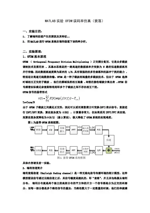
瑞利分布信道MATLAB仿真1、引言由于多径效应和移动台运动等影响因素,使得移动信道对传输信号在时间、频率和角度上造成了色散,即时间色散、频率色散、角度色散等等,因此多径信道的特性对通信质量有着重要的影响,而多径信道的包络统计特性则是我们研究的焦点。
根据不同无线环境,接收信号包络一般服从几种典型分布,如瑞利分布、莱斯分布等。
在此专门针对服从瑞利分布的多径信道进行模拟仿真,进一步加深对多径信道特性的了解。
2、仿真原理(1)瑞利分布分析环境条件:通常在离基站较远、反射物较多的地区,发射机和接收机之间没有直射波路径(如视距传播路径),且存在大量反射波,到达接收天线的方向角随机的((0~2π)均匀分布),各反射波的幅度和相位都统计独立。
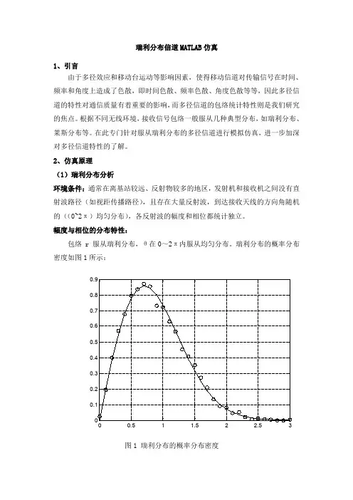
幅度与相位的分布特性:包络r服从瑞利分布,θ在0~2π内服从均匀分布。
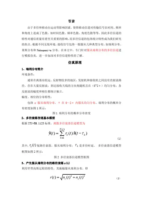
瑞利分布的概率分布密度如图1所示:图1瑞利分布的概率分布密度(2)多径衰落信道基本模型离散多径衰落信道模型为()1()()()N t k k k yt r t x t τ==-∑ (1)其中,()k r t 复路径衰落,服从瑞利分布;k τ是多径时延。
多径衰落信道模型框图如图2所示:图2多径衰落信道模型框图(3)产生服从瑞利分布的路径衰落r(t)利用窄带高斯过程的特性,其振幅服从瑞利分布,即()r t =(2)上式中()()c s n t n t 、,分别为窄带高斯过程的同相和正交支路的基带信号。
3、仿真框架根据多径衰落信道模型(见图2),利用瑞利分布的路径衰落r(t)和多径延时参数k τ,我们可以得到多径信道的仿真框图,如图3所示;图3多径信道的仿真框图4、仿真结果(1)(1)多普勒滤波器的频响图4多普勒滤波器的频响(2)多普勒滤波器的统计特性图5多普勒滤波器的统计特性(3)信道的时域输入/输出波形图6信道的时域输入/输出波形5、仿真结果(2)(1)当终端移动速度为30km/h时,瑞利分布的包络如下图所示(2)当终端移动速度为100km/h时,瑞利分布的包络如下图所示三、仿真代码%main.mclc;LengthOfSignal=10240;%信号长度(最好大于两倍fc)fm=512;%最大多普勒频移fc=5120;%载波频率t=1:LengthOfSignal;%SignalInput=sin(t/100);SignalInput=sin(t/100)+cos(t/65);%信号输入delay=[03171109173251];power=[0-1-9-10-15-20];%dBy_in=[zeros(1,delay(6))SignalInput];%为时移补零y_out=zeros(1,LengthOfSignal);%用于信号输出for i=1:6Rayl;y_out=y_out+r.*y_in(delay(6)+1-delay(i):delay(6)+LengthOfSignal-delay (i))*10^(power(i)/20);end;figure(1);subplot(2,1,1);plot(SignalInput(delay(6)+1:LengthOfSignal));%去除时延造成的空白信号title('Signal Input');subplot(2,1,2);plot(y_out(delay(6)+1:LengthOfSignal));%去除时延造成的空白信号title('Signal Output');figure(2);subplot(2,1,1);hist(r,256);title('Amplitude Distribution Of Rayleigh Signal')subplot(2,1,2);hist(angle(r0));title('Angle Distribution Of Rayleigh Signal');figure(3);plot(Sf1);title('The Frequency Response of Doppler Filter');%Rayl.mf=1:2*fm-1;%通频带长度y=0.5./((1-((f-fm)/fm).^2).^(1/2))/pi;%多普勒功率谱(基带)Sf=zeros(1,LengthOfSignal);Sf1=y;%多普勒滤波器的频响Sf(fc-fm+1:fc+fm-1)=y;%(把基带映射到载波频率)x1=randn(1,LengthOfSignal);x2=randn(1,LengthOfSignal);nc=ifft(fft(x1+i*x2).*sqrt(Sf));%同相分量x3=randn(1,LengthOfSignal);x4=randn(1,LengthOfSignal);ns=ifft(fft(x3+i*x4).*sqrt(Sf));%正交分量r0=(real(nc)+j*real(ns));%瑞利信号r=abs(r0);%瑞利信号幅值。
引言由于多径和移动台运动等影响因素,使得移动信道对传输信号在时间、频率和角度上造成了色散,如时间色散、频率色散、角度色散等等,因此多径信道的特性对通信质量有着至关重要的影响,而多径信道的包络统计特性成为我们研究的焦点。
根据不同无线环境,接收信号包络一般服从几种典型分布,如瑞利分布、莱斯分布和Nakagami-m 分布。
在本文中,专门针对服从瑞利分布的多径信道进行模拟仿真,进一步加深对多径信道特性的了解。
仿真原理1、瑞利分布简介 环境条件:通常在离基站较远、反射物较多的地区,发射机和接收机之间没有直射波路径,存在大量反射波;到达接收天线的方向角随机且在(0~2π)均匀分布;各反射波的幅度和相位都统计独立。
幅度、相位的分布特性:包络 r 服从瑞利分布,θ在0~2π内服从均匀分布。
瑞利分布的概率分布密度如图1所示:图1 瑞利分布的概率分布密度2、多径衰落信道基本模型根据ITU-RM.1125标准,离散多径衰落信道模型为()1()()()N t k k k y t r t x t τ==-∑%% (1)其中,()k r t 复路径衰落,服从瑞利分布; k τ是多径时延。
多径衰落信道模型框图如图2所示:图2 多径衰落信道模型框图3、产生服从瑞利分布的路径衰落r(t)利用窄带高斯过程的特性,其振幅服从瑞利分布,即()r t = (2)上式中,()c n t 、()s n t 分别为窄带高斯过程的同相和正交支路的基带信号。
首先产生独立的复高斯噪声的样本,并经过FFT 后形成频域的样本,然后与S (f )开方后的值相乘,以获得满足多普勒频谱特性要求的信号,经IFFT 后变换成时域波形,再经过平方,将两路的信号相加并进行开方运算后,形成瑞利衰落的信号r(t)。
如下图3所示:图3 瑞利衰落的产生示意图其中,()S f =(3) 4、 产生多径延时k τ 多径/延时参数如表1所示:表1 多径延时参数仿真框架根据多径衰落信道模型(见图2),利用瑞利分布的路径衰落r(t)(见图3)和多径延时参数k τ(见表1),我们可以得到多径信道的仿真框图,如图4所示;图4 多径信道的仿真框图仿真结果1、多普勒滤波器的频响图5多普勒滤波器的频响2、多普勒滤波器的统计特性图6 多普勒滤波器的统计特性3、信道的时域输入/输出波形图7信道的时域输入/输出波形小组分工程序编写:吴溢升报告撰写:谭世恒仿真代码%main.mclc;LengthOfSignal=10240; %信号长度(最好大于两倍fc)fm=512; %最大多普勒频移fc=5120; %载波频率t=1:LengthOfSignal; % SignalInput=sin(t/100);SignalInput=sin(t/100)+cos(t/65); %信号输入delay=[0 31 71 109 173 251];power=[0 -1 -9 -10 -15 -20]; %dBy_in=[zeros(1,delay(6)) SignalInput]; %为时移补零y_out=zeros(1,LengthOfSignal); %用于信号输出for i=1:6Rayl;y_out=y_out+r.*y_in(delay(6)+1-delay(i):delay(6)+LengthOfSignal-delay(i))*10^(power (i)/20);end;figure(1);subplot(2,1,1);plot(SignalInput(delay(6)+1:LengthOfSignal)); %去除时延造成的空白信号title('Signal Input');subplot(2,1,2);plot(y_out(delay(6)+1:LengthOfSignal)); %去除时延造成的空白信号title('Signal Output');figure(2);subplot(2,1,1);hist(r,256);title('Amplitude Distribution Of Rayleigh Signal')subplot(2,1,2);hist(angle(r0));title('Angle Distribution Of Rayleigh Signal');figure(3);plot(Sf1);title('The Frequency Response of Doppler Filter');%Rayl.mf=1:2*fm-1; %通频带长度y=0.5./((1-((f-fm)/fm).^2).^(1/2))/pi; %多普勒功率谱(基带) Sf=zeros(1,LengthOfSignal);Sf1=y;%多普勒滤波器的频响Sf(fc-fm+1:fc+fm-1)=y; %(把基带映射到载波频率)x1=randn(1,LengthOfSignal);x2=randn(1,LengthOfSignal);nc=ifft(fft(x1+i*x2).*sqrt(Sf)); %同相分量x3=randn(1,LengthOfSignal);x4=randn(1,LengthOfSignal);ns=ifft(fft(x3+i*x4).*sqrt(Sf)); %正交分量r0=(real(nc)+j*real(ns)); %瑞利信号r=abs(r0); %瑞利信号幅值。
Academic paper analysismatlab瑞利衰落信道仿真实习报告Academic paper analysisPaper: A Consolidated Architecture for 4G/B3G NetworksAuthors: M. Rubaiyat Kibria, Vinod Mirchandani, and Abbas Jamalipour Public: IEEE Communications Society / WCNC 20051.全文提纲outlineIn the paper,the authors briefly summarize current research in the architecture of fourth generation or beyond third generation (4G/B3G) network. At first, the author introduces the development of the next generation network and point that the operation of a fourth generation network will depend largely on the close coordination between mobility, resource and quality of service management schemes. Then the author briefly discusses three important techniques: Mobility Management, Resource Management and QoS Management during Handover. The author detailed describes the proposed architecture of network and mobile terminal by two thirds length of the paper. At the end of the article the author give some conclusions about 4G/B3G network.2.段落展开方式The way of the paragraphs outspread the way of the typicalscientific research article structures.First the current researches of this filed are introduced, thenthree parts are discussed separately. At the end, a conclusion isintroduced by the above discussion. At each paragraph, the first sentence of paragraph is topic sentence, then the following sentences talk about the topic.3.写作特点In my opinion, the most remarkable characteristic of this paper is that the hierarchy is very clear. The main idea of this paper is the architecture of next generation network. In order to discuss the architecture clearly, server important techniques are introduce firstly. In the main paragraphs, many proposed architectures are compared and are clearly describe one by one.4.重要句型被动语态:This paper is organized as follows:It is …使用:It is widely accepted that the next generation heterogeneous network will be all-IP based.as shown 使用:An underlying hierarchical structure, as shown in Fig. 3, is proposed to facilitate seamless mobility across heterogeneous networks. 5.重要单词4G/B3G:4G,B3G网络Internetworked Architecture:因特网工作体系结构Mobility Management:移动性管理Resource Management:资源分配管理Quality of Service(QOS):服务质量Bandwidth Broker:带宽管理Handover:切换6.习惯用法主谓搭配 Resource management requi res …动宾搭配 reduce battery power drain形容词与名词的搭配 dynamic link characteristics副词与动词的搭配 depend largely on介词与名词的搭配 on the QoS broker短语动词 is equipped with7.冠词的用法,时态的用法和其它首次提到使用A:A software defined radio (SDR) based reconfigurable mobile terminal (MT) provides access to such a scalable network. 指代整体使用The:The network architecture will be based on an Internet protocol version 6 (IPv6) underlying transport protocol that in effect will glue together thedifferent access networks.指代上文提到的使用This和These:This results in a considerable increase ofsignaling overhead.陈述一般情况用现在时:The main contribution in this paper is to proposeconsolidations in the above stated areas.已存在情况用现在完成时:Several 4G network architectures have been proposed byvarious researchers.陈述情况时使用被动语态:The network architecture will be based on an Internetprotocol version 6 (IPv6) underlying transport protocol that ineffect will glue together the different access networks.8.参考引用他人作品的方式(1)通过作者名字引用:From the several 4G architectures proposed inthe literature, we believe that the IST project Mobility and Differentiated Services in a Future IP Network (Moby Dick) [1] and Multimedia Integrated Network by Radio Access Innovation (MIRAI) [2] are the significant ones to have dealt with mobility management issue.(2)文章观点的引用:For example, [3] proposes a centralized bandwidth broker (BB) for each domain that considers the profile of each traffic encountered in the network and supports dynamic allocations.(3)项目直接引用,不提作者名:Other schemes such as Moby Dick project[4]propose a QoS broker, based on a hierarchical architecture.SMART/MIRAI [5] project suggests that differentiated flows should use heterogeneous networks based on the QoS requirements, but does not propose any resource management scheme in this regard.9.收获By reading this paper, I have learnt some improvement writing skills in formal English paper. First, I learnt the basic structure of a formal English paper and how to express your idea on the fixed structure. Second, I learnt that passive sentence is always used to describe thephenomenon already exists in formal paper. Third, I learnt how the tense used in academic paper. Last, I learnt how to reference other research in paper.。
瑞利分布信道MATLAB 仿真一、瑞利衰落原理在陆地移动通信中,移动台往往受到各种障碍物和其他移动体的影响,以致到达移动台的信号是来自不同传播路径的信号之和。
而描述这样一种信道的常用信道模型便是瑞利衰落信道。
定义:由于信号进行多径传播达到接收点处的场强来自不同传播的路径,各条路径延时时间是不同的,而各个方向分量波的叠加,又产生了驻波场强,从而形成信号快衰落称为瑞利衰落。
瑞利衰落信道(Rayleigh fading channel )是一种无线电信号传播环境的统计模型。
这种模型假设信号通过无线信道之后,其信号幅度是随机的,表现为“衰落”特性,并且多径衰落的信号包络服从瑞利分布。
由此,这种多径衰落也称为瑞利衰落。
这一信道模型能够描述由电离层和对流层反射的短波信道,以及建筑物密集的城市环境。
瑞利衰落只适用于从发射机到接收机不存在直射信号的情况,否则应使用莱斯衰落信道作为信道模型。
假设经反射(或散射)到达接收天线的信号为N 个幅值和相位均随机的且统计独立的信号之和。
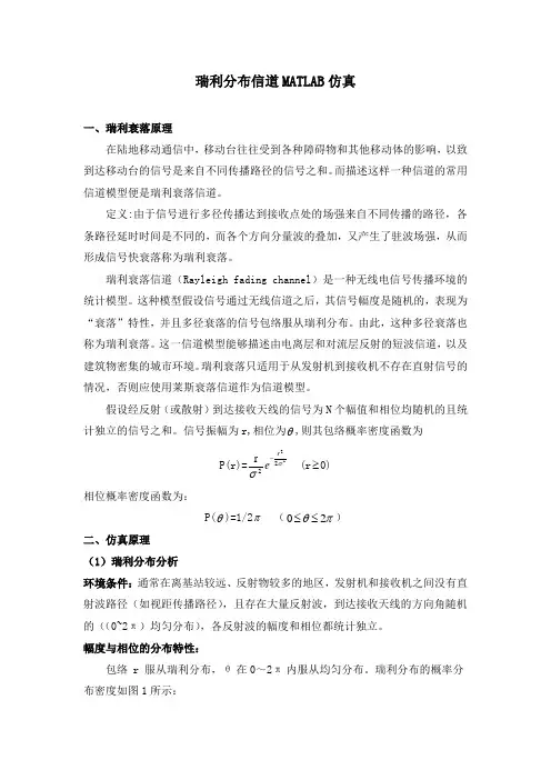
信号振幅为r,相位为θ,则其包络概率密度函数为 P(r)=2222r σσr e - (r ≥0)相位概率密度函数为:P(θ)=1/2π (πθ20≤≤)二、仿真原理(1)瑞利分布分析环境条件:通常在离基站较远、反射物较多的地区,发射机和接收机之间没有直射波路径(如视距传播路径),且存在大量反射波,到达接收天线的方向角随机的((0~2π)均匀分布),各反射波的幅度和相位都统计独立。
幅度与相位的分布特性:包络 r 服从瑞利分布,θ在0~2π内服从均匀分布。
瑞利分布的概率分布密度如图1所示:00.51 1.52 2.5300.10.20.30.40.50.60.70.80.9图1 瑞利分布的概率分布密度(2)多径衰落信道基本模型离散多径衰落信道模型为()1()()()N t k k k y t r t x t τ==-∑%% (1)其中,()k r t 复路径衰落,服从瑞利分布; k τ是多径时延。
瑞利信道Matlab仿真程序%%File_C7:Jakes.m%本程序将一随机信号通过瑞利信道产生输出%%clear;clc;Ts=0.02;fmax=2;%最大多普勒频移Nt=400;%采样序列的长度sig=j*ones(1,Nt);%信号t=[0:Nt];%设定信道仿真参数N0=25;D=1;[u]=jakes_single_rayleigh(N0,D,fmax,Nt,Ts);%生成瑞利信道RecSignal=u.*sig;plot(20*log10(RecSignal));%JakesRayleigh.m%本函数用Jakes方法产生单径的符合瑞利分布的复随机过程%%%%%%%%%%%%%%%%%%%%%%%%%%% function [u]=jakes_single_rayleigh(N0,D,fmax,M,Ts,Tc) % 输入参数:% N0 频率不重叠的正弦波个数% D 方差,可由输入功率得到% fmax 最大多普勒频移% M 码片数%输出参数%u 输出复信号%u1 输出信号的实部%u2 输出信号的虚部%%%%%%%%%%%%%%%%%%%%%%%%%%%%%N=4*N0+2;%Jakes仿真叠加正弦波的总个数%计算Jakes仿真中的离散多普勒频率fi,nf=zeros(1,N0+1);for n=1:N0f(n)=fmax*cos(2*pi*n/N);endf(N0+1)=fmax;%计算多普勒增益ci,n%同向分量增益c1,nc1=zeros(1,N0+1);for n=1:N0c1(n)=D*(2/sqrt(N))*2*cos(pi*n/N0); endc1(N0+1)=D*(2/sqrt(N))*sqrt(2)*cos(pi/4); %正交分量增益c2,nc2=zeros(1,N0+1);for n=1:N0c2(n)=D*(2/sqrt(N))*2*sin(pi*n/N0); endc2(N0+1)=D*(2/sqrt(N))*sqrt(2)*sin(pi/4); %插入随机相移ph_i,解决Jakes方法的广义平稳问题n=(1:N0+1);U=rand(size(n));[x,k]=sort(U);ph_i=2*pi*n(k)/(N0+1);%计算复包络u1=zeros(1,M);%Rc(t)u2=zeros(1,M);%Rs(t)u=zeros(1,M);%R(t)k=0;%计算Rc(t)k=0;for t=0:Ts:(M-1)*Ts;w2=cos(2*pi*f*t+ph_i); ut2=c2*w2.';k=k+1;u2(k)=ut2;end%计算u(t)k=0;for t=0:Ts:(M-1)*Tsk=k+1;u(k)=u1(k)-j*u2(k); end%程序结束。
Matlab瑞利信道仿真转眼间三⽉都已经过去⼀半,⼀直找不到有什么可以写的,⼀直想等⾃⼰把LTE仿真平台搭好后,再以连载的形式记录下来。
但是,后来⼀想,我必须先做好充分的铺垫,在这过程中也遇到了很多问题,及时留下点什么,也是好的。
即便以后回过头来再看这些⽂章,可能会有些许惊讶,惊讶于当时的⽆知或是稚嫩。
不得不说,时间真的是⼀把杀猪⼑,猪没少杀,更可怕的是扼杀了许多⼈的梦想。
今天没有去实验室,我觉得在忙了⼀周后,应该停下来歇歇,有时候的驻⾜观望或许是为了更好的前⾏。
⾔归正传,今天想记录的是⾃⼰在仿真中遇到的⼀个问题,那就是信道模型的仿真。
对于⽆线通信来说,最常见的就是瑞利衰落+多径+多普勒的模型了。
具体分析如下:瑞利衰落:就是有很多独⽴的⼩径的叠加,根据中⼼极限定理,知道这样的分布满⾜的是2个⾃由度的chi-square分布,也就是功率满⾜指数分布,幅度的分布就叫做瑞利分布。
它表明的是信道h的幅度和相位变化情况,幅度满⾜瑞利分布的变化,相位满⾜[0,2pi]上均匀分布的变化。
可以参考博⽂:多径效应:谈到多径效应,我们就应该想到频率选择性这个概念。
简单地说,就是延时的径在频域相当于相位搬移,每个径我们都可以看做是⼀个⽮量,幅度是由它们各⾃的功率决定,⾓度(相位)就是由每径延时决定。
然后,我们就做⽮量相加,最后得到的就是⼀个旋转⽮量,它对每个频率的响应都不同。
第⼆个概念就是,相⼲带宽:既然信道响应在各个频率点处的不同,那么我们关⼼的⼀个问题是,在多⼤的频率间隔上,它的响应是呈现⼀定的相关性(也就是说,在这个频率间隔上的响应变化⾮常慢,可以认为是相同的)。
这就很⾃然的过渡到功率延迟分布图上了,信道响应的频域(相关性)⽅⾯实质上是由信道时域的功率延迟分布做傅⽴叶变换得到的(功率与⾃相关函数的关系)。
功率延迟分布图是⼀个很有⽤的⼯具,我们能从中得到Trms(信道平均延迟,⽤功率去对延时加权)和Tmax(信道最⼤延时)等。
利用MATLAB仿真多径衰落信道利用MATLAB仿真多种多径衰落信道摘要:移动信道的多径传播引起的瑞利衰落,时延扩展以及伴随接收过程的多普勒频移使接受信号受到严重的衰落,阴影效应会是接受的的信号过弱而造成通信的中断:在信道中存在噪声和干扰,也会是接收信号失真而造成误码,所以通过仿真找到衰落的原因并采取一些信号处理技术来改善信号接收质量显得很重要,这里利用MATLAB对多径衰落信道的波形做一比较。
一,多径衰落信道的特点关于多径衰落信道,通过下面一个简单的模拟图来说明多径衰落信道的两个特点:频率选择性衰落和时间衰落。
dr0基站假设在一条笔直的高速公路上一段安装了一个固定的基站,另一端有一面完全反射的电磁波墙面。
当移动台静止时,显然从基站发出的直射信号到达移动台需要时间为r0/c,(c 为光速),从反射墙反射过来的信号到达移动台需要的时间为(2d-r0)/c。
也就是说,在t时刻,移动台接收分别接受了从时刻t-r0/c基站发出的直射信号和从时刻t-(2d-r0)/c基站发出的反射信号,而且信号在传播过程中要衰减,在自由空间中,直射信号和反射信号相位相反。
1,下面通过MATLAB画出在r0处接收信号会有什么特点:程序代码如下: clear allf=1; %发射信号频率v=1; %移动台速度,静止情况为0c=3e8; %电磁波速度,光速r0=3; %移动台距离基站初始距离d=10; %基站距离反射墙的距离t1=0.1:0.0001:10; %时间E1=cos(2*pi*f*((1-v/c).*t1-r0/c))./(r0+v.*t1); %直射径信号E2=cos(2*pi*f*((1+v/c)*t1+(r0-2*d)/c))./(2*d-r0-v*t1); %反射径信号figureplot(t1,E1,t1,E2,'-g',t1,E1-E2,'-r') %画出直射径、反射径和总的接收信号legend('直射径信号','反射径信号','移动台接收的合成信号')axis([0 10 -0.8 0.8])输出波形如下所示:由上图可以看出,即是移动台是静止的,由于反射径的存在,使得接收到的合成信号最大值要小于直射径信号:2,修改r0=9时,运行程序结果如下:通过上图我们可以看出,当r0=9时,由于靠墙比较近,直射信号要比r0=3处弱一些,反射信号要比r0=3强一些,但是移动台接收到的合成信号更弱了,不仅要小于直射径的信号,而且小于反射径的信号。
matlab多径瑞利衰落信道【原创实用版】目录1.多径瑞利衰落信道的概念和背景2.Matlab 在多径瑞利衰落信道仿真中的应用3.多径瑞利衰落信道仿真的重要性和挑战4.如何在 Matlab 中实现多径瑞利衰落信道的仿真5.总结与展望正文一、多径瑞利衰落信道的概念和背景多径瑞利衰落信道是一种无线通信信道模型,它描述了无线信号在传输过程中由于多径效应和瑞利衰落所引起的信号衰减和失真。
在城市密集区域、建筑物内部等环境中,无线信号会受到反射、折射、衍射等影响,导致信号强度的快速衰减和信道质量的恶化。
因此,研究多径瑞利衰落信道对于无线通信系统的设计和优化具有重要意义。
二、Matlab 在多径瑞利衰落信道仿真中的应用Matlab 是一种广泛应用于科学计算和工程设计的软件,其强大的数值计算和数据分析功能为多径瑞利衰落信道的仿真提供了便利。
在Matlab 中,可以通过编写自定义函数或使用现有的工具箱(如Communication Toolbox)来实现多径瑞利衰落信道的仿真。
三、多径瑞利衰落信道仿真的重要性和挑战多径瑞利衰落信道仿真对于无线通信系统的设计和优化具有重要意义,因为它可以帮助工程师了解系统在不同信道条件下的性能,从而指导系统参数的调整和优化。
然而,多径瑞利衰落信道仿真也面临着一些挑战,如信号模型的复杂性、参数设置的合理性、计算资源的需求等。
四、如何在 Matlab 中实现多径瑞利衰落信道的仿真在 Matlab 中实现多径瑞利衰落信道的仿真,可以采用如下步骤:1.创建信号模型:首先需要建立一个信号模型,描述信号在多径瑞利衰落信道中的传播过程。
这可以通过编写自定义函数或使用现有的工具箱来实现。
2.设置系统参数:在进行仿真之前,需要设置一些系统参数,如信号的调制方式、传输速率、信道带宽等。
这些参数的设置会影响到仿真结果的准确性和可靠性。
3.编写仿真代码:根据信号模型和系统参数,可以编写 Matlab 代码来实现多径瑞利衰落信道的仿真。
m a t l a b瑞利衰落信道仿真 Prepared on 24 November 2020
引言
由于多径和移动台运动等影响因素,使得移动信道对传输信号在时间、频率和角度上造成了色散,如时间色散、频率色散、角度色散等等,因此多径信道的特性对通信质量有着至关重要的影响,而多径信道的包络统计特性成为我们研究的焦点。
根据不同无线环境,接收信号包络一般服从几种典型分布,如瑞利分布、莱斯分布和Nakagami-m 分布。
在本文中,专门针对服从瑞利分布的多径信道进行模拟仿真,进一步加深对多径信道特性的了解。
仿真原理
1、瑞利分布简介 环境条件:
通常在离基站较远、反射物较多的地区,发射机和接收机之间没有直射波路径,存在大量反射波;到达接收天线的方向角随机且在(0~2π)均匀分布;各反射波的幅度和相位都统计独立。
幅度、相位的分布特性:
包络 r 服从瑞利分布,θ在0~2π内服从均匀分布。
瑞利分布的概率分布密度如图1所示:
图1 瑞利分布的概率分布密度
2、多径衰落信道基本模型
根据标准,离散多径衰落信道模型为
()
1
()()()
N t k k k y t r t x t τ==-∑ (1)
其中,()k r t 复路径衰落,服从瑞利分布; k τ是多径时延。
多径衰落信道模型框图如图2所示:
图2 多径衰落信道模型框图
3、产生服从瑞利分布的路径衰落r(t)
利用窄带高斯过程的特性,其振幅服从瑞利分布,即
()r t = (2)
上式中,()c n t 、()s n t 分别为窄带高斯过程的同相和正交支路的基带信号。
首先产生独立的复高斯噪声的样本,并经过FFT 后形成频域的样本,然后与S (f )开方后的值相乘,以获得满足多普勒频谱特性要求的信号,经IFFT 后变换成时域波形,再经过平方,将两路的信号相加并进行开方运算后,形成瑞利衰落的信号r(t)。
如下图3所示:
图3 瑞利衰落的产生示意图
其中,
()S f =
(3) 4、
产生多径延时k τ
多径/延时参数如表1所示:
表1 多径延时参数
仿真框架
根据多径衰落信道模型(见图2),利用瑞利分布的路径衰落r(t)(见图
(见表1),我们可以得到多径信道的仿真框图,如图4 3)和多径延时参数k
所示;
图4 多径信道的仿真框图
仿真结果
1、多普勒滤波器的频响
图5多普勒滤波器的频响
2、多普勒滤波器的统计特性
图6 多普勒滤波器的统计特性
3、信道的时域输入/输出波形
图7信道的时域输入/输出波形
小组分工
程序编写:吴溢升
报告撰写:谭世恒
仿真代码
%
clc;
LengthOfSignal=10240; %信号长度(最好大于两倍fc)
fm=512; %最大多普勒频移
fc=5120; %载波频率
t=1:LengthOfSignal; % SignalInput=sin(t/100);
SignalInput=sin(t/100)+cos(t/65); %信号输入
delay=[0 31 71 109 173 251];
power=[0 -1 -9 -10 -15 -20]; %dB
y_in=[zeros(1,delay(6)) SignalInput]; %为时移补零
y_out=zeros(1,LengthOfSignal); %用于信号输出
for i=1:6
Rayl;
y_out=y_out+r.*y_in(delay(6)+1-delay(i):delay(6)+LengthOfSignal-delay(i))*10^(power(i)/20);
end;
figure(1);
subplot(2,1,1);
plot(SignalInput(delay(6)+1:LengthOfSignal)); %去除时延造成的空白信号title('Signal Input');
subplot(2,1,2);
plot(y_out(delay(6)+1:LengthOfSignal)); %去除时延造成的空白信号
title('Signal Output');
figure(2);
subplot(2,1,1);
hist(r,256);
title('Amplitude Distribution Of Rayleigh Signal')
subplot(2,1,2);
hist(angle(r0));
title('Angle Distribution Of Rayleigh Signal');
figure(3);
plot(Sf1);
title('The Frequency Response of Doppler Filter');
%
f=1:2*fm-1; %通频带长度
y=./((1-((f-fm)/fm).^2).^(1/2))/pi; %多普勒功率谱(基带)
Sf=zeros(1,LengthOfSignal);
Sf1=y;%多普勒滤波器的频响
Sf(fc-fm+1:fc+fm-1)=y; %(把基带映射到载波频率)
x1=randn(1,LengthOfSignal);
x2=randn(1,LengthOfSignal);
nc=ifft(fft(x1+i*x2).*sqrt(Sf)); %同相分量
x3=randn(1,LengthOfSignal);
x4=randn(1,LengthOfSignal);
ns=ifft(fft(x3+i*x4).*sqrt(Sf)); %正交分量
r0=(real(nc)+j*real(ns)); %瑞利信号
r=abs(r0); %瑞利信号幅值。