DCO_2 on-line measurement used in rapamycin fed-batch fermentation process

DC1705A-BD ESCRIPTIONUltralow Noise and Spurious Integer-N Frequency Synthesizer with Integrated VCODC1705A features the L TC®6946, an ultralow noise and spurious integer-N frequency synthesizer with integrated VCO. The VCO uses no external components and is inter-nally calibrated without external system support. There are three versions of the DC1705A, one for each version of the L TC6946. The DC1705A-A contains the L TC6946-1, the DC1705A-B incorporates the L TC6946-2 and DC1705A-C uses the L TC6946-3.Each DC1705A provides 50Ω SMA connectors for the reference frequency input, f REF, the reference output buffer (REF OUT), and the differential RF output (RF+ and RF–).A DC590 USB serial controller board is used for SPI com-munication with the L TC6946, controlled by the supplied PLLWizard™ software.Design files for this circuit board are available at /demoL, L T, L TC, L TM, Linear Technology and the Linear logo are registered trademarks and PLLWizard and QuikEval are trademarks of Linear Technology Corporation. All other trademarks are the property of their respective owners.Figure 1. Proper Measurement Equipment Setup1dc1705afaDEMO MANUAL DC1705APARAMETER INPUT OR OUTPUT PHYSICAL LOCATION DETAILS3.3V Power Supply Input 3.3V and GND Banana Jacks Low Noise and Spur-Free 3.3V, 115mA5V Power Supply Input5V and GND Banana Jacks Low Noise and Spur-Free 5V, 45mAREF+ IN, Reference Frequency Input J1 SMA Connector Low Noise 10MHz or 100MHz*, 6dBm into 50Ω(Note 1)REF OUT, Buffered Reference Output J3 SMA Connector Frequency = f REF, 0dBmRF+ and RF–T wo Outputs J4 and J5 SMA Connectors Frequency: 900MHz*, Power: 0dBm, FrequencyRange: Depends on the version of the L TC6946device – refer to Table 1, Step Size: 200kHz* Loop Bandwidth–Set by Loop Filter Component Values47kHz** These frequencies are for the DC1705A pllset files included with PLLWizard.Note 1: A low noise 10MHz or 100MHz reference frequency, such as the Wenzel 501-04608A or 501-04516D OCXO, is recommended. If using a different frequency, make sure to update the f REF and R_DIV boxes under the System tab in PLLWizard so that f PFD is still 1MHz. For example, if a 20MHz clock is used, f REF should be changed to 20MHz and R_DIV to 20. REF BST and FIL T under the System tab in PLLWizard might need to be changed if the reference frequency and/or power is different than what is recommended in the table above. More information can be found in the LTC6946 data sheet.Table 1. DC1705A Options and Frequency RangesASSEMBL Y VERSION PART NUMBER VCO FREQUENCY RANGE (GHz)OUTPUT DIVIDER SETTINGSDC1705A-A L TC6946IUFD-1 2.240 to 3.740Integers 1 through 6DC1705A-B L TC6946IUFD-2 3.080 to 4.910Integers 1 through 6DC1705A-C L TC6946IUFD-3 3.840 to 5.790Integers 1 through 6T YPICAL DC1705A REQUIREMENTS AND CHARACTERISTICSQ UICK START PROCEDUREThe DC590 and PLLWizard application are required to control the DC1705A through a personal computer (PC). DC590 ConfigurationThe DC590’s QuikEval™ drivers must be installed before the DC590 will be able to communicate with the L TC6946. To configure the DC590, follow the procedure below, start-ing with step 1. If you have already installed the DC590 software previously, skip to step 5.Note: Once the QuikEval software is installed, the applica-tion does not need to be executed to run PLLWizard or to control the DC1705A.1. Do Not plug in the DC590 before running the installation program.2. Download the QuikEval installation program from /software.3. Run the QuikEval installation program and follow the on-screen instructions. More detailed installation infor-mation may be found in the DC590’s Quick Start guide.4. Exit the QuikEval program once the installation is com-plete, as it is not needed to run the PLLWizard software.5. Place the DC590 jumpers in the following positions: JP4EE Must be in the “EN” position.JP5ISO ”ON” must be selected.JP5SW ”ON” must be selected.JP6VCCIO “3.3V” must be selected. This sets the SPI port to 3.3V operation.6. Connect the DC590 to one of your computer’s USB ports with the included USB cable.2dc1705afaDEMO MANUAL DC1705AFigure 2. DC590 Jumper LocationsQUICK START PROCEDUREPLLWizard InstallationThe PLLWizard software is used to communicate with the L TC6946 synthesizer. It uses the DC590 to translate between USB and SPI-compatible serial communications formats. It also includes advanced PLL design and simula-tion capabilities. The following are the PLLWizard system requirements:• Windows Operating System: Windows XP, Windows 2003 Server, Windows Vista, Windows 7• Microsoft .NET 2.0 or later• Windows Installer 3.1 or later• Linear Technology’s QuikEval and DC590 hardware Microsoft .NETYou must have Microsoft .NET 2.0 or later installed on your computer. PLLWizard will not run without it. Note that with Windows Vista and Windows 7 have at least version 3.5 pre-installed.To manually determine your version of .NET using Win-dows XP, click Start Menu→Settings→Control Panel →Add or Remove Programs.Depending upon your .NET version, choose one of two PLLWizard setup programs, downloaded from /software.3dc1705afa4dc1705afaDEMO MANUAL DC1705A QUICK START PROCEDUREFigure 3. PLLWizard ScreenshotEither setup program will automatically install Microsoft .NET if a compatible .NET version is not found. But, the installation source depends upon which file you down-loaded from Linear Technology’s website. You should pick one of the following two choices, depending upon your version of .NET .Table 2. PLLWizard Installation FileFILE.NET 2.0 SOURCEPLLWizardSetup.exe Latest Version Downloaded from Microsoft PLLWizardSetup_net20.exe2.0 SP2 Included (Much Larger File Size)• Choose PLLWizardSetup if you have .NET 2.0 or later , have Windows Vista or Windows 7, or if you have less than .NET 2.0 but want the latest .NET installed.• Choose PLLWizardSetup_net20 if you have less than .NET 2.0, and want faster installation (no additional Microsoft downloads are needed, but the file size is much larger).The setup file will verify and/or install Microsoft .NET and install PLLWizard. Refer to the Help menu for softwareoperation.DEMO MANUAL DC1705A QUICK START PROCEDUREDC1705A Configuration1. Connect an appropriate reference frequency source (at J1) and signal analyzers (at J4 and/or J5) using the SMA connectors (see Figure 1 and the Typical DC1705A Requirements and Characteristics table).2. Choose the MUTE jumper setting: JP1 - GND/3.3V MUTE position. Select GND to mute the RF output, 3.3V to un-mute.3. Connect the GND, 3.3V and 5V banana jacks to a power supply and apply power (see Figure 1 and the Typical DC1705A Requirements and Characteristics table).4. Connect the DC590 to the DC1705A with the provided ribbon cable.5. Run the PLLWizard application.6. In PLLWizard, click File → Load Settings and point to the appropriate pllset file. For example, if you are using a 10MHz reference with a DC1705A-B to evaluate the L TC6946-2, load the “DC1705A-B (L TC6946-2) 10MHz Ref.pllset” file found in the PLLWizard installation direc-tory (typically Program Files → L TC → PLLWizard →Set Files).The red LED on DC1705A should turn on indicating that the loop is locked at 900MHz.You can then change the values of N_DIV and/or O_DIV in PLLWizard to change the output frequency.T roubleshootingIf the red LED does not illuminate, follow the instructions below:1. Verify that you are able to communicate with the DC1705A. The bottom status line in PLLWizard should read “L TC6946” and “Comm Enabled.” Refer to PLL-Wizard’s T roubleshoot and Help if not.2. Verify that the3.3V and 5V have the correct voltages on them and that the reference frequency is applied to the REF+ IN SMA input.If the red LED is on but you cannot detect an RF output, make sure jumper JP1 is at the 3.3V position. Run Help →T roubleshoot in PLLWizard if the problem is not resolved. DC1705A ReconfigurationYou can redesign the frequency plan of the DC1705A using PLLWizard. You can change the loop filter components as found using PLLWizard by reinstalling the loop filter components shown in Figure 4.Figure 4. DC1705A Components and Connections5dc1705afaDEMO MANUAL DC1705AP ARTS LISTITEM QTY REFERENCE PART DESCRIPTION MANUFACTURER/PART NUMBERDC1705A General BOM11CI1 Capacitor, X7R 0.022μF 50V 5% 0603AVX 06035C223JAT2A21CI2Capacitor, COG 6800pF 50V 5% 0805Murata GRM2195C1H682JA01D31CP Capacitor, COG 2700pF 50V 5% 0603Murata GRM1885C1H272JA01D44C1, C8, C9, C18Capacitor, X7R, 1μF, 16V, 10%, 0805TDK, C2012X7R1C105K52C2, C10Capacitor, Tantalum, 330μF, 10V, 10%, 7343AVX, TPME337K010R003562C6, C11Capacitor, X7R, 470pF, 50V, 10%, 0402AVX, 04025C471KAT2ACapacitor, X7R, 0.01μF, 16V, 10%, 0402AVX, 0402YC103KAT2A 74C7, C12, C15,C198C13, C14, C17,Capacitor, X5R, 0.1μF, 10V, 10%, 0402TDK, C1005X5R1A104KC22, C23,8C24, C25, C2691C16Capacitor, X7R, 2.2μF, 16V, 10%, 0805TDK, C2012X7R1C225K102C20, C21Capacitor, NPO, 100pF, 50V, 5%, 0402TDK, C1005C0G1H101J111D1LED, Red Panasonic, LN1251CTR124E1, E2, E5, E8Jack, Banana Keystone, 575-4131E3Turret, Testpoint, 2501 Mill-Max, 2501-2-00-80-00-00-07-0141JP1Headers, 3 Pins 2mm Ctrs.Samtec TMM-103-02-L-S151XJP1Shunt, 2mm Ctrs.Samtec 2SN-BK-G164J1, J3, J4, J5Connector, SMA 50Ω EDGE-LAUNCH E. F. Johnson, 142-0701-851171J2Connector, Header, 14-Pin, 2mm Molex, 87831-1420182L1, L2Inductor, Chip, 68nH, ±5%, 0402 Coilcraft, 0402 HPH-68NXJL191RZ Resistor, Chip, 453 1/10W 1% 0603NIC, NRC06F4530TRF201R1Resistor, Chip, 51.1Ω, 1/16W, 1% 0402NIC, NRC04F51R1TRF211R3Resistor, Chip, 330Ω, 1/16W, 1% 0402NIC, NRC04F3300TRF221R4Resistor, Chip, 15Ω, 1/16W, 1% 0402NIC, NRC04F15R0TRF234R5, R6, R7, R13Resistor, Chip, 200k, 1/16W, 1% 0402NIC, NRC04F2003TRF242R8, R9Resistor, Chip, 4.99k, 1/16W, 1% 0402NIC, NRC04F4991TRF253R10, R11, R12Resistor, Chip, 100Ω 1/16W, 5%, 0402NIC, NRC04J101TRF262U2, U3IC, Dual Buffer SC-70 6-Lead Fairchild Semi. NC7WZ17P6X271U4 IC, Dual T ransceiver SC-70 6-Lead NXP 74LVC1T45GW284 4 Corners Standoff, Nylon, 0.5, 1/2"Keystone, 8833 (SNAP ON)DC1705A-A11DC1705A General BOM DC1705A21U1IC Synthesizer QFN-28 4mm × 5mm Linear Technology Corporation, L TC6946IUFD-1DC1705A-B11DC1705A General BOM DC1705A21U1IC Synthesizer QFN-28 4mm × 5mm Linear Technology Corporation, L TC6946IUFD-2DC1705A-C11DC1705A General BOM DC1705A21U1IC Synthesizer QFN-28 4mm × 5mm Linear Technology Corporation, L TC6946IUFD-36dc1705afa7dc1705afaDEMO MANUAL DC1705ASCHEMATIC DIAGRAM8dc1705afaDEMO MANUAL DC1705A SCHEMATIC DIAGRAMNote: The buffers shown on sheet 2 of 2 of the schematic are used to protect the L TC6946 when communicating to it starts before powering it up. There is no need for such circuitry if the SPI bus is not active before powering up the LTC6946.9dc1705afaDEMO MANUAL DC1705AInformation furnished by Linear Technology Corporation is believed to be accurate and reliable.However , no responsibility is assumed for its use. Linear Technology Corporation makes no representa-tion that the interconnection of its circuits as described herein will not infringe on existing patent rights.L AYOUT The top metal layer of the DC1705A is shown here as an example of good PCB layout for the L TC6946.10dc1705afa DEMO MANUAL DC1705ALinear Technology Corporation 1630 McCarthy Blvd., Milpitas, CA 95035-7417(408) 432-1900 ● FAX: (408) 434-0507 ● www.linear .com © LINEAR TECHNOLOGY CORPORA TION 2011LT 1211 REV A • PRINTED IN USADEMONSTRATION BOARD IMPORTANT NOTICELinear Technology Corporation (L TC) provides the enclosed product(s) under the following AS IS conditions:This demonstration board (DEMO BOARD) kit being sold or provided by Linear Technology is intended for use for ENGINEERING DEVELOPMENT OR EVALUATION PURPOSES ONL Y and is not provided by L TC for commercial use. As such, the DEMO BOARD herein may not be complete in terms of required design-, marketing-, and/or manufacturing-related protective considerations, including but not limited to product safety measures typically found in finished commercial goods. As a prototype, this product does not fall within the scope of the European Union directive on electromagnetic compatibility and therefore may or may not meet the technical requirements of the directive, or other regulations.If this evaluation kit does not meet the specifications recited in the DEMO BOARD manual the kit may be returned within 30 days from the date of delivery for a full refund. THE FOREGOING WARRANTY IS THE EXCLUSIVE WARRANTY MADE BY THE SELLER TO BUYER AND IS IN LIEU OF ALL OTHER WARRANTIES, EXPRESSED, IMPLIED, OR STATUTORY, INCLUDING ANY WARRANTY OF MERCHANTABILITY OR FITNESS FOR ANY PARTICULAR PURPOSE. EXCEPT TO THE EXTENT OF THIS INDEMNITY, NEITHER PARTY SHALL BE LIABLE TO THE OTHER FOR ANY INDIRECT , SPECIAL, INCIDENTAL, OR CONSEQUENTIAL DAMAGES.The user assumes all responsibility and liability for proper and safe handling of the goods. Further , the user releases L TC from all claims arising from the handling or use of the goods. Due to the open construction of the product, it is the user’s responsibility to take any and all appropriate precautions with regard to electrostatic discharge. Also be aware that the products herein may not be regulatory compliant or agency certified (FCC, UL, CE, etc.).No License is granted under any patent right or other intellectual property whatsoever. L TC assumes no liability for applications assistance, customer product design, software performance, or infringement of patents or any other intellectual property rights of any kind.L TC currently services a variety of customers for products around the world, and therefore this transaction is not exclusive .Please read the DEMO BOARD manual prior to handling the product . Persons handling this product must have electronics training and observe good laboratory practice standards. Common sense is encouraged .This notice contains important safety information about temperatures and voltages. For further safety concerns, please contact a L TC applica-tion engineer .Mailing Address:Linear Technology1630 McCarthy Blvd.Milpitas, CA 95035Copyright © 2004, Linear Technology CorporationDC1705A-B。

DC-II™DROP CELL / DIP CELL OPERATION MANUALTable of contents1. Overview32. Scope 43. Equipment requirements44. Calibration instructions55. Measurement66. Notes12List of tablesTable 1 Normal cathodic protection rangesfor bare carbon steel in seawater 7 Table 2 Troubleshooting 8List of figuresFigure 1 Calibration cell-to-cell 9 Figure 2 Calibration vs. zinc coupon 10 Figure 3 Cable immersion test 11Notes:1. Specifications subject to change without notice2. Platforms and risers must be inspected via drop cell yearly in the Gulf ofMexico per API RP 2A-WSD as part of Level I inspections1. OverviewThe DC-II™ drop-cell is a dual element silver/silver chloride (Ag/AgCl) reference electrode for measuring cathodic protection potentials in seawater; readings are taken with a multi-meter . The reference electrode cable has two leads, one to each element. The bare ends of the wires should never be immersed in water .The DC-II™ is lowered into the seawater off the side of a platform or vessel. The slender, weighted body reduces the chance that the DC-II™ could become entangled in the struc-ture or surrounding objects. The DC-II™ is lowered to the deter-mined water depth(s) and the structure potential is recorded from a hand-held multi-meter .Reference electrode elements in housingStandard 250’ reelDC20004Optional 500’ reelDC200222.0 ScopeThe purpose of this document is to instruct users on how to properly operate the DC-II™, including general assembly, recording andinterpreting potential readings.3.0 Equipment requirementsOne of each of the following is needed. Please note that it’s wise tohave a spare of each.3.1 DC II™ + spooled cable3.2 Multi-meter (preferably intrinsically safe)3.3 Test leads, alligator-type (usually attached to multi-meter) 3.4 Metal file or rasp3.5 Zinc calibration coupon with lead wire (calibration only)3.6 Pencil or pen3.7 Clipboard or notepad for recording potentialreadings and depths3.8 Grounding cable with large alligator clip (optional)3.9 Gas meter (optional)3.10Non-metallic bucket (calibration only)3.11Valid certificate of calibration for the multi-meter (usuallyattached to the multi-meter)4.0 Calibration instructions (See Figure 1)CAUTIONAlways inspect test leads, connectors and drop cell cable for cracksor breaks in the insulation before each use. If any defects are found,replace item immediately. Ensure that the test leads do not get wet.4.1 Check test leads on multi-meter:4.1.1Connect both test leads to the multi-meter: One to the “V-Ω” terminal and the other to the “COM” terminal.4.1.2Set the multi-meter to the smallest resistance scale (typically 200 Ohms).4.1.3Ground the probe end of the test leads together and record the value. If this value is 0.5 Ohms or less, proceed. Ifthis value is greater than 0.5 Ohms, check test leads fordamage and retest; otherwise, replace the test leads.4.2 Fill a non-metallic bucket or container with enough seawateror simulated seawater solution to fully immerse the DC-II™, verifying that the water is free of oil.4.3 Insert the DC-II™ into the seawater and agitate the DC-II™ toremove all air bubbles. This ensures that the Ag/AgCl referenceelectrodes are in contact with seawater.4.4 Clean the zinc calibration coupon with a file or sandpaper.Remove most of the oxide layer and insert the coupon into bucket,leaving the lead wire above water.4.5 Allow the DC-II™ to soak for approximately one hour to allowthe electrodes to reach equilibrium (usually not necessary if probehas been used recently).4.6 Set the multi-meter to the 200mV DC scale.4.7 Take a reading between the two Ag/AgCl reference elements(The two bare wires from the DC-II™). The reading on the metershould have a value of +/- 10.0mV or less. If so, the survey mayproceed. If the reading is greater than +/- 10.0mV, soak theelectrodes for another hour to reach equilibrium and check again. Ifreading is still not within +/- 10.0mV, the DC-II™ should be replaced.4.8Set the multi-meter to the 2.0V DC scale. (See Figure 2)4.9 Take a reading between the zinc calibration coupon’s leadwire and each Ag/AgCl reference element (a total of two readings) as shown in Figure 2.4.10The value on the meter for each reading should be between (-) 1.030 V and (-) 1.070 V (depending on the purity of the zinc coupon).5.0MeasurementCAUTIONA hot work permit may be required If the multi-meter being used isnot intrinsically safe, as a multi-meter is considered a spark hazard.5.1Deploy the DC-II™ housing into the seawater to the first depthspecified (usually 3 meters [10 feet]).5.2Connect the multi-meter test lead from the “COM” terminal toeither of the two Ag/AgCl electrode leads.5.3Using a steel file or rasp, remove coating and corrosionproduct from a very small area of the structure down to bare metal.The area to be used must be electrically continuous with the mainstructure. Some sections of grating may only be fastened to the deck by bolting and should not be used.5.4Connect the multi-meter test lead from the “V-Ω” terminal tothe uncoated portion of the structure (from the previous step).5.5Set the multi-meter to the 2 volt DC scale.5.6Record the potential reading from the multi-meter and waterdepth into a notebook or form.5.7Record the multi-meter reading at each depth increment of5m, or as required.5.8After the last reading, disconnect the multi-meter and coil thecable evenly onto the reel.5.9Soak the elements in a non-metallic bucket of fresh water forat least one hour before storing.Table 1 - Normal cathodic protection ranges for bare carbon steel in seawaterNote: For brackish or fresh water, please consult Peterson’s Nomogram.VoltmeterMFR0038Troubleshooting the DC-II™Table 2 -Notes:1. Never allow the leads to contact the structure directly.2. Only connect through a high-impedence multimeter.3. To avoid entanglement, always deploy on the down stream / downwind.Figure 1CELL TO CELL CALIBRATION DC-II™ CALIBRATION WIRING SCHEMATICNote: To avoid damaging the cable, do not invert the DC-II™ when placing it in the bucket.Figure 2CELL TO ZN COUPONDC-II™ CALIBRATION WIRING SCHEMATICVoltmeter display at 2.0V DC setting should be within -1.030V and -1.070 V. Readings outside this range indicate possible damage to wire on spool.Note: Clean the Zn coupon with a file or sandpaper before using.Note: Clean the Zn coupon with a file or sandpaper before using.Figure 3CABLE IMMERSION TEST CHECKING DC-II™ CABLE FOR DEFECTSWithout a Zn coupon, you can determine if a cable is defective. Pull lengths of cable through the bucket; when the readings sud-denly shift, you’ve found the defect. Use an undam-aged probe for the survey instead.Voltmeter to leads With the voltmeter display at 2.0V DC setting, feed lengths of cable through the bucket. Any nicks will cause a noticeable shift in the voltmeter readings. Do this individually with each wire within the cable. If the damage is isolated to only one wire, readings can still be taken using the unaffected lead if no other undamaged probe is ing a Zn couponNOTES。

Office of Research and DevelopmentUNITED STATES ENVIRONMENTAL PROTECTION AGENCYNATIONAL EXPOSURE RESEARCH LABORATORYHUMAN EXPOSURE & ATMOSPHERIC SCIENCES DIVISION (MD-D205-03)Research Triangle Park, NC 27711919-541-5691Issue Date : October 12, 2011(/ttn/amtic/criteria.html)These methods for measuring ambient concentrations of specified air pollutants have been designated as "reference methods" or "equivalent methods" in accordance with Title 40, Part 53 of the Code of Federal Regulations (40 CFR Part 53). Subject to any limitations (e.g., operating range or temperature range) specified in the applicable designation, each method is acceptable for use in state or local air quality surveillance systems under 40 CFR Part 58 unless the applicable designation is subsequently canceled. Automated methods for pollutants other than PM 10 are acceptable for use only at shelter temperatures between 20°C and 30°C and line voltages between 105 and 125 volts unless wider limits are specified in the method description.Prospective users of the methods listed should note (1) that each method must be used in strict accordance with its associated operation or instruction manual and with applicable quality assurance procedures, and (2) that modification of a method by its vendor or user may cause the pertinent designation to be inapplicable to the method as modified. (See Section 2.8 of Appendix C, 40 CFR Part 58 for approval of modifications to any of these methods by users.)Further information concerning particular designations may be found in the Federal Register notice cited for each method or by writing to the National Exposure Research Laboratory, Human Exposure and Atmospheric Sciences Division (MD-D205-03), U.S. Environmental Protection Agency, Research Triangle Park, North Carolina 27711. Technical information concerning the methods should be obtained by contacting the source listed for each method. Source addresses are listed at the end of the listing of methods, except for the addresses for lead method sources, which are given with the method. New analyzers or PM 10 samplers sold as reference or equivalent methods must carry a label or sticker identifying them as designated methods. For analyzers or PM 10 or samplers sold prior to the designation of a method with the same or similar model number, the model number does not necessarily identify an analyzer or sampler as a designated method. Consult the manufacturer or seller to determine if a previously sold analyzer or sampler can be considered a designated method or if it can be upgraded to designation status. Analyzer users who experience operational or other difficulties with a designated analyzer or sampler and are unable to resolve the problem directly with the instrument manufacturer may contact EPA (preferably in writing) at the above address for assistance.This list will be revised as necessary to reflect any new designations or any cancellation of a designation currently in effect. The most current revision of the list will be available for inspection at EPA's Regional Offices, and copies may be obtained at the Internet site identified above or by writing to the National Exposure Research Laboratory at the address specified above.TSP List of Designated Reference and Equivalent Methods, October 12, 2011 Page 3Reference Method for TSPManual Reference Method: 40 CFR Part 50, Appendix BReference Method for the Determination of Suspended Particulate Matter in the Atmosphere (High-Volume Method) Federal Register: Vol. 47, page 54912, 12/06/82 and Vol. 48, page 17355, 04/22/83Andersen Model RAAS10-100 PM10 Single Channel PM10 SamplerManual Reference Method: RFPS-0699-130“Andersen Instruments, Incorporated Model RAAS10-100 Single Channel Reference Method PM10Sampler,” wi th RAAS-10 PM10 inlet or the louvered inlet specified in 40 CFR 50 Appendix L, Figs. L-2 thru L-19, configured as a PM10 reference method, and operated for 24-hour continuous sample periods at a flow rate of 16.67 liters/ minute, and in accordance with the Model RAAS105-100 Operator‟s Manual and with the requirements and sample collection filters specified in 40 CFR Part 50, Appendix J or Appendix M.Federal Register: Vol. 64, page 33481, 06/23/99Andersen Model RAAS10-200 PM10 Single Channel PM10 Audit SamplerManual Reference Method: RFPS-0699-131“Andersen Instruments, Incorporated Model RAAS10-200 Single Channel Reference Method PM10Audit Sampler,” with RAAS-10 PM10 inlet or the louvered inlet specified in 40 CFR 50 Appendix L, Figs. L-2 thru L-19, configured as a PM10 reference method, and operated for 24-hour continuous sample periods at a flow rate of 16.67 liters/minute, and in accordance with the Model RAAS105-200 Operator‟s Manual and with the requirements and sample collection filters specified in 40 CFR Part 50, Appendix J or Appendix M.Federal Register: Vol. 64, page 33481, 06/23/99Andersen Model RAAS10-300 PM10 Multi Channel PM10 SamplerManual Reference Method: RFPS-0699-132“Andersen Instruments, Incorporated Model RAAS10-300 Multi Channel Sequential Reference Method PM10Sampler,” with RAAS-10 PM10 inlet or the louvered inlet specified in 40 CFR 50 Appendix L, Figs. L-2 thru L-19, configured as a PM10 reference method, and operated for 24-hour continuous sample periods at a flow rate of 16.67 liters/minute, and in accordance with the Model RAAS105-300 Operator‟s Manual and with the requirements and sample collection filters specified in 40 CFR Part 50, Appendix J or Appendix M.Federal Register: Vol. 64, page 33481, 06/23/99BGI Incorporated Model PQ100 Air SamplerManual Reference Method: RFPS-1298-124“BGI Incorporated Model PQ100 Air Sampler,” with BGI 16.7 Inlet Kit or the louvered inlet specified in 40 CFR 50 Appendix L, Figs. L-2 thru L-19, configured as a PM10 reference method, for 24-hour continuous sample periods at a flow rate of 16.7 liters/minute, with original firmware Version 5.X and lower or new firmware version 6.0 and higher, operated in accordance with the original Model PQ100 Instruction Manual or manual revision Version 7.0, as appropriate, and with the requirements specified in 40 CFR Part 50, Appendix J or Appendix M, using either the original or the newer PQ200-type filter cassettes, and with or without the optional Solar Panel Power Supply.Federal Register: Vol. 63, page 69625, 12/17/98Latest modification: 01/2009BGI Incorporated Model PQ200 Air SamplerManual Reference Method: RFPS-1298-125“BGI Incorporated Model PQ200 Air Sampler,” with “flat plate” PM10inlet or the louvered inlet specified in 40 CFR 50 Appendix L, Figs. L-2 thru L-19, configured as a PM10reference method, and operated for 24-hour continuous sample periods in accordance with the Model PQ200 Instruction Manual and with the requirements specified in 40 CFR Part 50, Appendix J or Appendix M, and with or without the optional Solar Panel Power Supply.Federal Register: Vol. 63, page 69625, 12/17/98DKK-TOA Models FPM-222/222C, FPM223/223C, and DUB-222(S)/223(S) PM10 MonitorAutomated Equivalent Method: EQPM-0905-156“DKK-TOA Models FPM-222, FPM-222C, FPM-223, FPM-223C, DUB-222(S), and DUB-223(S) Particulate Monitor,” for monitoring PM10in Ambient Air (beta attenuation monitor), configured for PM10, with Firmware Version DUB4-658355, Corrected Slope Factor (FACT SLOPE) set to 1.232, Corrected Zero Value (FACT ZERO) set to 1.8, and with or without any of the following options: Auto Check and Serial Recorder.Federal Register: Vol. 70, page 56684, 09/28/05Ecotech Model 3000 PM10 High Volume Air SamplerManual Reference Method: RFPS-0706-162“Ecotech Pt y. Ltd. Model 3000 PM10High Volume Air Sampler,” configured with the Ecotech PM10Size-Selective Inlet (SSI)(P-ECO-HVS3000-02), with the flow rate set to 1.13 m3/min (67.8 m3/hour).Federal Register: Vol. 71, page 42089, 07/25/06Environnement S.A. Model MP101M PM10 MonitorAutomated Equivalent Method: EQPM-0404-151“Environnement S. A. Model MP101M PM10Beta Gauge Monitor,” configured with the louvered PM10 inlet specified in 40 CFR 50 Appendix L or its flat-topped predecessor version and one of the three optional temperature-regulated sampling tubes (RST), and operated with a full scale measurement range of 0 - 0.500 mg/m3 (0 - 500 g/m3), with the sample flow rate set to 1.00 m3/h and flow regulation set to yes, the “norms selection” set to m3 (actual v olume), the “cycle” set to 24 hours, the “period” set to none, and the “counting time” set to 200 seconds.2Federal Register: Vol. 69, page 18569, 4/8/04Graseby Andersen/GMW Model 1200 High-Volume Air SamplerManual Reference Method: RFPS-1287-063“Sierra-Andersen or General Metal Works Model 1200 PM10High-Volume Air Sampler System," consisting of a Sierra-Andersen or General Metal Works Model 1200 PM10 Size-Selective Inlet and any of the high-volume air samplers identified as SAUV-10H, SAUV-11H, GMW-IP-10, GMW-IP-10-70, GMW-IP-10-801, or GMW-IP-10-8000, which include the following components: Anodized aluminum high-volume shelter with either acrylonitrile butadiene styrene plastic filter holder and motor/blower housing or stainless steel filter holder and phenolic plastic motor/blower housing; 0.6 hp motor/blower; pressure transducer flow recorder; either an electronic mass flow controller or a volumetric flow controller; either a digital timer/programmer, seven-day mechanical timer, six-day timer/programmer, or solid-state timer/programmer; elapsed time indicator; and filter cartridge.Federal Register: Vol. 52, page 45684, 12/01/87 and Vol. 53, page 1062, 01/15/88Graseby Andersen/GMW Model 321-B High-Volume Air SamplerManual Reference Method: RFPS-1287-064"Sierra-Andersen or General Metal Works Model 321-B PM10 High-Volume Air Sampler System," consisting of a Sierra-Andersen or General Metal Works Model 321-B PM10 Size-Selective Inlet and any of the high-volume air samplers identified as SAUV-10H, SAUV-11H, GMW-IP-10, GMW-IP-10-70, GMW-IP-10-801, or GMW-IP-10-8000, which include the following components: Anodized aluminum high-volume shelter with either acrylonitrile butadiene styrene plastic filter holder and motor/blower housing or stainless steel filter holder and phenolic plastic motor/blower housing; 0.6 hp motor/blower; pressure transducer flow recorder; either an electronic mass flow controller or a volumetric flow controller; either a digital timer/programmer, seven-day mechanical timer, six-day timer/programmer, or solid-state timer/programmer; elapsed time indicator; and filter cartridge.Federal Register: Vol. 52, page 45684, 12/01/87 and Vol. 53, page 1062, 01/15/88Graseby Andersen/GMW Model 321-C High-Volume Air SamplerManual Reference Method: RFPS-1287-065"Sierra-Andersen or General Metal Works Model 321-C PM10 High-Volume Air Sampler System," consisting of a Sierra-Andersen General Metal Works Model 321-C PM10 or Size-Selective Inlet and any of the high-volume air samplers identified as SAUV-10H, SAUV-11H, GMW-IP-10, GMW-IP-10-70, GMW-IP-10-801, or GMW-IP-10-8000, which include the following components: Anodized aluminum high-volume shelter with either acrylonitrile butadiene styrene plastic filter holder and motor/blower housing or stainless steel filter holder and phenolic plastic motor/blower housing; 0.6 hp motor/blower; pressure transducer flow recorder; either an electronic mass flow controller or a volumetric flow controller; either a digital timer/programmer, seven-day mechanical timer, six-day timer/programmer, or solid-state timer/programmer; elapsed time indicator; and filter cartridge.Federal Register: Vol. 52, page 45684, 12/01/87 and Vol. 53, page 1062, 01/15/88Graseby Andersen/GMW Models SA241 and SA241M Dichotomous SamplerManual Reference Method: RFPS-0789-073“Sierra-Andersen Models SA241 and SA241M or General Metal Works Models G241 and G241M PM10Dichotomous Samplers,” consisting of the following components: Sampling Module with SA246b or G246b 10 m inlet or the louvered inlet specified in 40 CFR 50 Appendix L, Figs. L-2 thru L-19, 2.5 m virtual impactor assembly, 37 mm coarse and fine particulate filter holders, and tripod mount; Control Module with diaphragm vacuum pump, pneumatic constant flow controller, total and coarse flow rotameters and vacuum gauges, pressure switch (optional), 24-hour flow/event recorder, digital timer/programmer or 7-day skip timer, and elapsed time indicator.Federal Register: Vol. 54, page 31247, 07/27/89Graseby Andersen/GMW Model FH621-N Beta MonitorAutomated Equivalent Method: EQPM-0990-076“Andersen Instruments Model FH62I-N PM10Beta Attenuation Monitor,”consisting of the following components: FH101 Vacuum Pump Assembly; FH102 Accessory Kit; FH107 Roof Flange Kit; FH125 Zero and Span PM10 Mass Foil Calibration Kit; FH62I Beta Attenuation 19-inch Control Module; SA246b PM10 Inlet (16.7 liter/min) or the louvered inlet specified in 40 CFR 50 Appendix L, Figs. L-2 thru L-19; operated for 24-hour average measurements, with an observing time of 60 minutes, the calibration factor set to 2400, a glass fiber filter tape, an automatic filter advance after each 24-hour sample period, and with or without either of the following options: FH0P1 Indoor Cabinet; FH0P2 Outdoor Shelter Assembly.Federal Register: Vol. 55, page 38387, 09/18/90Met One or Sibata Models BAM/GBAM 1020, BAM/GBAM 1020-1 or Horiba APDA-371Automated Equivalent Method: EQPM-0798-122“Met One Instruments or Sibata Scientific Technology Models BAM 1020, GB AM 1020, BAM 1020-1, GBAM 1020-1, and Horiba APDA-371 PM10Beta Attenuation Monitor,” including the BX-802 sampling inlet, operated for 24-hour average measurements, with a filter change frequency of one hour, with glass fiber filter tape, and with or without any of the following options: BX-823, tube extension; BX-825, heater kit; BX-826, 230 VAC heater kit; BX-827 “Smart Heater” set for maintaining moisture between 35% and 45% and no ΔT control; BX-828, roof tripod; BX-902, exterior enclosure; BX-903, exterior enclosure with temperature control; BX-961, mass flow controller; BX-967, internal calibration device, BX-970 touch-screen display with USB interface. For software (firmware) versions V3.0 or higher, a user-selectable measurement time (COUNT TIME) of 4, 6, 8 or 10 minutes selected, along with appropriate sample time (BAM SAMPLE) setting of 50, 46, 42 or 38 minutes, respectively, to maintain a 60-minute measurement cycle. For software (firmware) versions V3.5 or higher, user-selectable option to sample under actual conditions (Flow Type: ACTUAL) and report under standard conditions (Reporting: STD), which requires the use of P/N BX-592 external temperature sensor or P/N BX-596 external temperature/barometric pressure sensor. The user may also sample under standard conditions (Flow Type: STD) and report under standard conditions (Reporting: STD) with any software/firmware 2.0 or higher. Instrument must be operated in accordance with the appropriate instrument manual.Federal Register: Vol. 63, page 41253, 08/03/98Latest modifications: 06/2009; 07/2010; 8/2010Opsis Model SM200 PM10 MonitorAutomated Equivalent Method: EQPM-0810-193“O psis Model SM200 Monitor,” beta gauge semi-continuous ambient particulate monitor operated for 24 hours at a flow rate of 16.67 LPM between 5° and 40°C using 47 mm PTFE membrane filter media, in the mass measurement range of 0 to 60 mg, configured with a BGI Model SSI25 PM10inlet meeting criteria specified in 40 CFR 50 Appendix L, with a roof mounting kit, and with or without an inlet tube heater (as recommended based on site RH conditions), according to the SM200 User‟s Guide.Federal Register: Vol. 75, page 51039, 08/18/10Oregon DEQ Medium Volume PM10 SamplerManual Reference Method: RFPS-0389-071“Oregon DEQ Medium Volume PM10 Sampler.” NOTE: This method is no longer commercially available.Federal Register: Vol. 54, page 12273, 03/24/89Thermo Andersen Series FH 62 C14 Continuous PM10 MonitorThermo Scientific Model 5014i Beta (5014i Beta), Continuous Ambient Particulate MonitorAutomated Equivalent Method: EQPM-1102-150“Thermo Andersen Series FH 62 C14 Continuous PM10Ambient Particulate Monitor and Thermo Scientific Model 5014i Beta (5014i Beta), Continuous Ambient Particulate Monitor,” operated for 24-hour average measurements, with the specified 10-micron inlet, inlet connector, sample tube with heater, roof flange kit, mass foil kit, pump kit, sample filter tape; with operational settings of 1000 L/h (16.67 L/min) sample flow rate, daily filter change, auto filter change at volumetric flow <950 L/h, auto filter change at mass >1500 micrograms, and factory default calculation mode settings operated with software version 1.07. Operated, calibrated and serviced according to the appropriate Operator Manual.Federal Register: Vol. 67, page 76174, 12/11/02Latest modification: 07/2009Thermo Scientific or Rupprecht & Patashnick Partisol® Model 2000 Air SamplerManual Reference Method: RFPS-0694-098“Thermo Scientific Partisol®2000 Air Sampler” or “Rupprecht & Patas hnick Partisol® Model 2000 Air Sampler," consisting of a Hub Unit and 0, 1, 2, or 3 Satellite Units, with each sampling station used for PM10measurements equipped with a Rupprecht & Patashnick PM10inlet and operated for continuous 24-hour periods using the Basic, Manual, Time, Analog Input, or Serial Input programming modes, and with or without any of the following options: PM2.5-style filter cassette holder; louvered inlet specified in 40 CFR 50 Appendix L, Figs. L-2 thru L-19 in lieu of standard inlet; 57-002320 Stand for Hub or Satellite; 59-002542 Advanced EPROM; 10-001403 Large Pump (1/4 hp); 120 VAC. Hardware for Indoor Installation consists of: 51-002638-xxxx Temperature Sensor (Extended Length); 55-001289 Roof Flange (1 1/4"); 57-000604 Support Tripod for Inlet; 57-002526-0001 Sample Tube Extension (1 m); 57-002526-0002 Sample Tube Extension (2 m). Hardware for Outdoor Installation in Extreme Cold Environments consists of: 10-002645 Insulating Jacket for Hub Unit.Federal Register: Vol. 59, page 35338, 07/11/94Thermo Scientific Partisol®2000-D Dichotomous Air Sampler or Thermo Fisher Scientific Partisol®2000i-D Dichotomous Air SamplerManual Equivalent Method: EQPS-0311-197“Thermo Scientific Partisol®2000-D Dichotomous Air Sampler” or “Thermo F isher Scientific Partisol®2000i-D Dichotomous Air Sampler,”configured for dual-filter, single-event sampling of fine (PM2.5) and coarse (PM10-2.5) particles, operated with a U.S. EPA PM10inlet and using a virtual impactor to separate fine and coarse PM into two samples for collection on two separate filter membranes, for a 24-hour sampling period and in accordance with the Partisol® 2000-D or Partisol® 2000i-D instruction manual, as appropriate. Partisol® 2000i-D operated with firmware version 2.0 or greater. Federal Register: Vol. 76, page 15974, 03/22/11Latest modification: 06/2011Thermo Scientific Partisol® 2000-FRM PM10 Air Sampler or Thermo Fisher Scientific Partisol® 2000i PM10 Air Sampler or Rupprecht and Patashnick Partisol®-FRM 2000 PM10 Air SamplerManual Reference Method: RFPS-1298-126“Thermo Scientific Partisol® 2000-FRM PM10Air Sampler” or “Thermo Fisher Scientific Partisol® 2000i PM10 Air Sampler”or “Rupprecht and Patashnick Partisol®-FRM 2000 PM10Air Sampler,” with PM10 inlet or louvered inlet specified in 40 CFR 50, Appendix L, Figs. L-2 through L-19, configured as a PM10 reference method with a U.S. EPA PM10 inlet with straight downtube adapter and operated for 24-hour continuous sampling periods in accordance with the Partisol® 2000-FRM or Partisol® 2000i instruction manual,as appropriate, and with the requirements specified in 40 CFR Part 50, Appendix J or Appendix M. Model 2000i operated with firmware version 2.0 or greater.Federal Register: Vol. 63, page 69625, 12/17/98Latest modification: 06/ 2011PM10List of Designated Reference and Equivalent Methods, October 12, 2011 Page 8 Thermo Scientific Partisol®-Plus 2025 PM10Sequential Air Sampler or Thermo Fisher Scientific Partisol®2025i PM10 Sequential Air Sampler or Rupprecht and Patashnick Partisol®-Plus 2025 PM10 Sequential Air SamplerManual Reference Method: RFPS-1298-127“Thermo Scientific Partisol®-Plus 2025 Sequential Air Sampler” or “Thermo Fisher Scientific Partisol® 2025i Sequential Air Sampler”or “Rupprecht and Patashnick Partisol®-Plus 2025 PM10Sequential Air Sampler,” with PM10 inlet or louvered inlet specified in 40 CFR 50, Appendix L, Figs. L-2 through L-19, configured as a PM10 reference method and operated for 24-hour continuous sampling periods. Partisol®-Plus2025 to be operated with any software version 1.003 through 1.5 and the Partisol® 2025i with firmware version 2.0 or greater, with the modified filter shuttle mechanism, in accordance with the Partisol®-Plus 2025 or Partisol® 2025i instruction manual, as appropriate, and with the requirements specified in 40 CFR Part 50, Appendix J or Appendix M.Federal Register: Vol. 63, page 69625, 12/17/98Last modified: 06/ 2011Thermo Scientific Dichotomous Partisol®-Plus 2025-D Sequential Air Sampler or Thermo Fisher Scientific Dichotomous Partisol® 2025i-D Sequential Air SamplerManual Equivalent Method: EQPS-0311-198“Thermo Scientific Dichotomous Partisol®-Plus 2025-D Sequential Air Sampler” or “Thermo Fisher Scientific Dichotomous Partisol® 2025i-D Sequential Air Sampler,” configured for dual-filter sampling of fine (PM2.5) and coarse (PM10-2.5) particles, with a U.S. EPA PM10 inlet and using a virtual impactor to separate the fine and coarse PM into two samples for collection on two separate filter membranes, and operated with the modified filter shuttle mechanism implemented May 31, 2008, and firmware version 1.500 or greater for the Partisol®-Plus 2025-D and version 2.0 or greater for the Partisol® 2025i-D, for 24-hour continuous sampling periods, in accordance with the Partisol®-Plus 2025-D or Partisol® 2025i-D instruction manual, as appropriate.Federal Register: Vol. 76, page 15975, 03/22/11Latest modification: 06/ 2011Thermo Scientific TEOM® 1400AB/TEOM® 1405 Ambient Particulate Monitor orRupprecht & Patashnick TEOM® Series 1400/1400a PM10 MonitorsAutomated Equivalent Method: EQPM-1090-079“Thermo Scientific TEOM® 1400AB [PM10] Ambient Particulate Monitor” or “Rupprecht & Patashnick TEOM® Series 1400 and Series 1400a PM-10 Monitors,” (including serial number prefixes 1400, 140A, 140AA, 140AB, 140AT, and 140UP, 1405A), consisting of the following components: TEOM®Sensor Unit; TEOM®Control Unit; Flow Splitter (3 liter/min sample flow); Teflon-Coated Glass Fiber Filter Cartridges; Rupprecht & Patashnick PM-10 Inlet (part number 57-00596), Sierra-Andersen Model 246b PM-10 Inlet (16.7 liter/min) or louvered inlet specified in 40 CFR 50 Appendix L, Figs. L-2 thru L-19; operated for 24-hour average measurements, with the total mass averaging time set at 300 seconds, the mass rate/mass concentration averaging time set at 300 seconds, the gate time set at 2 seconds, and with or without any of the followingoptions: Tripod; Outdoor Enclosure; Automatic Cartridge Collection Unit (Series 1400a only); Flow Splitter Adapter (for 1 or 2 liter/min sample flow). Thermo Scientific TEOM® 1405 Ambient Particulate Monitor with combined sensor and control units and redesigned mass transducer and user interface, operated in accordance with the Thermo Scientific TEOM® 1405 instrument manual.Federal Register: Vol. 55, page 43406, 10/29/90Latest modification: 12/2008Tisch Environmental Model TE-6070 PM10 High-Volume Air Sampler or New Star Environmental Model NS-6070 PM10 High-Volume Air SamplerManual Reference Method: RFPS-0202-141“Tisch Environmental Model TE-6070 or New Star Environmental Model NS-6070 PM10High-Volume Air Sampler,” consisting of a TE-6001 PM10 size-selective inlet, 8" x 10" filter holder, aluminum outdoor shelter, mass flow controller or volumetric flow controller with brush or brushless motor, 7-day mechanical off/on-elapsed timer or 11-day digital off/on-elapsed timer, and any of the high volume sampler variants identified as TE-6070-BL or NS-6070-BL, TE-6070D or NS-6070D, TE-6070D-BL or NS-6070-BL, TE-6070V or NS-6070V, TE-6070V-BL or NS-6070V-BL, TE-6070-DV or NS-6070-DV, or TE-6070DV-BL or NS-6070DV-BL, with or without the optional stainless steel filter media holder/filter cartridge or continuous flow/pressure recorder.Federal Register: Vol. 67, page 15566, 04/02/02Wedding & Associates' or Thermo Environmental Instruments Inc. Model 600 PM10 High-Volume SamplerManual Reference Method: RFPS-1087-062"Wedding & Associates' or Thermo Environmental Instruments, Inc. Model 600 PM10 Critical Flow High-Volume Sampler," consisting of the following W&A/TEII components: PM10 Inlet; Critical Flow Device; Anodized Aluminum Shelter; Blower Motor Assembly for 115, 220 or 240 VAC and 50/60 Hz; Mechanical Timer; Elapsed Time Indicator; and Filter Cartridge/Cassette, and with or without the following options: Digital Timer, 6 or 7 Day Timer, and 1 or 7 Day Pressure Recorder.Federal Register: Vol. 52, page 37366, 10/06/87Wedding & Associates' or Thermo Environmental Instruments Inc. Model 650 PM10 Beta GaugeAutomated Equivalent Method: EQPM-0391-081“Wedding & Associates' or Thermo Environmental Instruments, Inc. Model 650 PM10Beta Gauge Automated Particle Sampler,” consisting of the following W&A/TEII components: Particle Sampling Module, PM10 Inlet (18.9 liter/min), Inlet Tube and Support Ring, Vacuum Pump (115, 220 or 240 VAC and 50/60 Hz); and operated for 24-hour average measurements with glass fiber filter tape.Federal Register: Vol. 56, page 9216, 03/05/91Andersen Model RAAS2.5-200 PM2.5 Ambient Audit Air SamplerManual Reference Method: RFPS-0299-128“Andersen Instruments, Incorporated Model RAAS2.5-200 PM2.5Audit Sampler,” configured as a PM2.5 reference method and operated with software (firmware) version 4B, 5.0.1 - 6.09, 6.0A, or 6.0B, for 24-hour continuous sample periods at a flow rate of 16.67 liters/minute, and in accordance with the Model RAAS2.5-200 Operator‟s Manual and with the requirements and sample collection filters specified in 40 CFR Part 50, Appendix L.Federal Register: Vol. 64, page 12167, 03/11/99BGI Inc. Models PQ200 or PQ200A PM2.5 Ambient Fine Particle SamplerManual Reference Method: RFPS-0498-116“BGI Incorporated Models PQ200 and PQ200A PM2.5Ambient Fine Particle Sampler,” operated with firmware version 3.88 or 3.89R, for 24-hour continuous sample periods, in accordance with the Model PQ200/PQ200A Instruction Manual and with the requirements and sample collection filters specified in 40 CFR Part 50, Appendix L, and with or without the optional Solar Power Supply or the optional dual-filter cassette (P/N F-21/6) and associated lower impactor housing (P/N B2027), where the upper filter is used for PM2.5. The Model PQ200A is described as a portable audit sampler and includes a set of three carrying cases.Federal Register: Vol. 63, page 18911, 04/16/98BGI Inc. Models PQ200-VSCC™ or PQ200A-VSCC™ PM2.5 SamplerManual Reference Method: RFPS-0498-116 or Manual Equivalent Method: EQPM-0202-142“BGI Incorporated Models PQ200-VSCC™ or PQ200A-VSCC™ PM2.5Ambient Fine Particle Sampler,” configured with a BGI VSCC™ Very Sharp Cut Cyclone particle size separator and operated with firmware version 3.88, 3.91, 3.89R, or 3.91R, for 24-hour continuous sample periods, in accordance with the Model PQ200/PQ200A Instruction Manual and VSCC™supplemental manual and with the requirements and sample collection filters specified in 40 CFR Part 50, Appendix L, and with or without the optional Solar Power Supply or the optional dual-filter cassette (P/N F-21/6) and associated lower impactor housing (P/N B2027), where the upper filter is used for PM2.5. The Model PQ200A VSCC™is described as a portable audit sampler and includes a set of three carrying cases.Federal Register: Vol. 67, page 15567, 04/02/02Graseby Andersen Model RAAS2.5-100 PM2.5 Ambient Air SamplerManual Reference Method: RFPS-0598-119“Graseby Andersen Mo del RAAS2.5-100 PM2.5Ambient Air Sampler,” operated with software version 4B, 5.0.1 - 6.09, 6.0A, or 6.0B, configured for “Single 2.5” operation, for 24-hour continuous sample periods at a flow rate of 16.67 liters/minute, and in accordance with the Model RAAS2.5-100 Operator‟s Manual and with the requirements and sample collection filters specified in 40 CFR Part 50, Appendix L.Federal Register: Vol. 63, page 31991, 06/11/98Graseby Andersen Model RAAS2.5-300 PM2.5 Sequential Ambient Air SamplerManual Reference Method: RFPS-0598-120“Graseby Andersen Model RAAS2.5-300 PM2.5Sequential Ambient Air Sampler,” operated with software version 4B, 5.0.1 - 6.09, 6.0A, or 6.0B, configured for “Multi 2.5" operation, for 24-hour continuous sample periods at a flow rate of 16.67 liters/minute, and in accordance with the Model RAAS2.5-300 Operator‟s Manual and with the requirements and sample collection filters specified in 40 CFR Part 50, Appendix L.Federal Register: Vol. 63, page 31991, 06/11/98Grimm Model EDM 180 PM2.5 MonitorAutomated Equivalent Method: EQPM-0311-195“Grimm Technologies, Inc. Model EDM 180 PM2.5Monitor,” light scattering continuous ambient particulate monitor operated for 24 hours at a volumetric flow rate of 1.2 L/min, configured with a Nafion®-type air sample dryer, complete for operation with firmware version 7.80 or later, in accordance with the Grimm Technologies, Inc. Model EDM 180 Operation and Instruction Manual. The optional graphic presentation can be made with the software model 1.177 version 3.30 or later. Federal Register:Vol. 76, page 15974, 03/22/11。

T echnical DataFluke 123 IndustrialScopeMeterSpecificationsIntroductionPerformance characteristics Fluke guarantees the properties expressed in numerical values with the stated tolerance.Specified non-tolerance numeri-cal values indicate those that could be nominally expected from the mean of a range of identical ScopeMeter test tools.Environmental data The environmental datamentioned in this technical data are based on the results of the manufacturer’s verification procedures.Safety characteristicsThe ScopeMeter 123 test tool has been designed and tested in accordance with ANSI/ISA S82.01-1994, EN 61010.1 (1993)(IEC 1010-1), CAN/CSA-C22.2No.1010.1-92, UL3111-1 Safety Requirements for Electrical Equipment for Measurement,Control, and Laboratory e of this equipment in a manner not specified by the manufacturer may impair protection provided by the equipment.SpecificationsDual input oscilloscope VerticalFrequency response DC coupled:Excluding probes and test leads:DC to 20 MHz (-3 dB)With STL120 1:1 shielded test leads:DC to 12.5 MHz (-3 dB)DC to 20 MHz (-6 dB)With PM 8918 10:1 probe (optional accessory): DC to 20 MHz (-3 dB)AC coupled (LF roll off)Excluding probes and test leads:<10 Hz (-3 dB)With STL120: <10 Hz (-3 dB)With PM 8918: <1 Hz (-3 dB)Rise timeExcluding probes and test leads:<17.5 nsInput impedanceExcluding probes and test leads:1 M Ω//12 pFWith BB120: 1 M Ω//20 pF With STL120: 1 M Ω//225 pF With PM 8918: 10 M Ω//15 pF Sensitivity: 5 mV to 500V/div Display modes: A, -A, B, -B Max input voltageA, B: 600V rms up to 200 kHz,derating to 6V rms @ 20 MHz Max floating voltageFrom any terminal to ground:600V rms up to 400 Hz Resolution: 8 bitVertical accuracy: ±(1% of reading + 0.05 range/div)Max vertical move: ±4 divisionsHorizontalAcquisition modesNormal: Equivalent sampling: 20 ns to 500 ns/div; real time sampling:1 µs to 5s/divSingle (real time): 1 µs to 5s/div Roll (real time): 1s to 60s/div Sampling rate (for both channels simultaneously): For repetitivesignals (equivalent sampling) up to 1.25 GS/s; real time (normal and single): 1 µs to 5 ms/div, 25 MS/s;10 ms to 5s/div, 5 MS/s Time base accuracyEquivalent sampling: ±(0.4%of reading +0.04 time/div)Real time sampling: ±(0.1%of reading +0.04 time/div)Glitch detection: ≥40 ns@ 20 ns to 5 ms/div; ≥200 ns @ 10 ms to 5s/divGlitch detection is always active Horizontal move, 10 divisions.Permits shifting of the displayfrom 0 to 10 division of pre-trigger.Trigger point will always be visible.®1981TriggerMode: Auto, Triggered, Single Source: A, B, EXT. EXTernal via optically isolated trigger probeITP120 (optional accessory) Sensitivity A and B@ DC to 5 MHz: 0.5 divisions or 5 mV @ 25 MHz: 1.5 divisions@ 40 MHz: 4 divisionsSlope: Positive, NegativeVideo A and BModes: Lines, Line Select Standards: NTSC, PAL, PAL+, SECAM Polarity: Positive, Negative Sensitivity: 0.6 divisions sync Advanced scope functions Display modesNormal: Captures up to 40 ns glitches and displays analog-like persistence waveformSmooth: Removes noise from a waveformEnvelope: Records and displays the minimum and maximum of wave-forms over timeConnect-and-View TM Continuous fully automatic adjustment of amplitude, time base, trigger levels, trigger gap, hold-off, and position.Manual override: Manual adjust-ment of amplitude, time base, trigger level, or position.Dual inputautoranging meterThe accuracy of all measurements is within ±(% of reading + number of counts) from 18°C to 28°C.Add 0.1x (specific accuracy) for each °C below 18°C or above 28°C. For voltage measurements with 10:1 probe, add probe uncertainty +1%. At least one waveform period must be visible on the screen. Input A and Input BDC Voltage (VDC)Ranges:500 mV, 5V, 50V, 500V, 1250V Accuracy:±(0.5% +5 counts) Normal mode rejection (SMR):>60 dB @ 50 or 60 HzCommon mode rejection (CMRR): >100 dB @ dc; >60 dB @ 50, 60, or 400 HzResolution: 5000 counts True-rms voltages(VAC and VAC+DC)Ranges:500 mV, 5V, 50V, 500V, 1250VAccuracy for 5% to 100% of rangeDC coupled: DC to 60 Hz (VAC+DC)±(1% +10 counts);1 Hz to 60 Hz(VAC) ±(1% +10 counts)AC or DC coupled: 60 Hz to 20 kHz±(2.5% +15 counts); 20 kHz to1 MHz ±(5% +20 counts); 1 MHzto 5 MHz ±(10% +25 counts); 5 MHzto 20 MHz ±(30% +25 counts)AC coupled with 1:1 (shielded)test leads: 60 Hz (6 Hz with 10:1probe) -1.5%; 50 Hz (5 Hz with10:1 probe) -2%; 33 Hz (3.3 Hzwith 10:1 probe) -5%; 10 Hz(1 Hz with 10:1 probe) -30%Normal mode rejection (SMR):>60 dB @ 50 or 60 Hz ±1%Common mode rejection (CMRR):>100 dB @ dc; >60 dB @ 50, 60,or 400 HzResolution: 5000 countsCrest factor: Automatic rangingon crest factor overloadPeakModes: Max peak, Min peak, orpk-to-pkRanges: 50 mV, 500 mV, 5V, 50V,500V, 1250VAccuracy: Max peak or Min peak,5% of full scale; peak-to-peak,10% of full scaleResolution: 500 countsFrequency (Hz)Ranges: 1 Hz, 10 Hz, 100 Hz, 1 kHz,10 kHz, 100 kHz, 1 MHz, 10 MHz,40 MHz (1 Hz and 10 Hz in manualmode or Auto Set LF ranging only)Accuracy: @ dc to 1 MHz, ±(0.5%+2 counts); @1 MHz to 10 MHz±(1.0% +2 counts); @10 MHz to40 MHz ±(2.5% +2 counts)Resolution: 1000 countsDuty Cycle (DUTY)Range: 2% to 98%Accuracy: Same as frequencyResolution: 0.1%Pulse Width (PULSE)Accuracy: Same as frequencyResolution: 1000 countsAmperes (AMP)With optional current probeRanges: Same as VDC, VAC,VAC+DC, or peakScale factor: 1 mV/A, 10 mV/A,100 mV/A, and 1 V/AAccuracy: Same as VDC, VAC,VAC+DC, or peak (add currentprobe uncertainty)Temperature (TEMP)With optional temperature probeRange: Same as VDCScale Factor: 1 mV/°C and 1 mV/°FAccuracy: Same as VDC (addtemperature probe uncertainty)Decibel (dB)0 dBV: 1V0 dBm (600Ω/50Ω): 1 mWreferenced to 600Ω or 50Ω dBon VDC, VAC, or VAC+DCResolution: 1000 countsCrest Factor (CREST)Range: 1 to 10Accuracy:±(5% +1 count)Resolution: 100 countsPhaseModes: A to B, B to ARange: 0 to 359°Accuracy:±(1° +1 count)Resolution: 1°Input AOhm (Ω)Ranges: 500Ω, 5 kΩ, 50 kΩ,500 kΩ, 5 MΩ, 30 MΩAccuracy:±(0.6% +5 counts)Resolution: 5000 countsMeasurement current: 0.5 mA to50 nA (decreases with increasingranges)Open circuit voltage: <4VContinuity (CONT)Beep: <(30Ω±5Ω) in 50Ω rangeMeasurement current: 0.5 mADetection of shorts of:≥1 msDiodeMaximum voltage: @ 0.5 mA 2.8V;@ open circuit 4VAccuracy:±(2% +5 counts)Measurement current: 0.5 mAPolarity: + on input A, - on COMCapacitance (CAP)Ranges: 50 nF, 500 nF, 5 µF,50 µF, 500 µFAccuracy:±(2% +10 counts)Resolution: 5000 countsMeasurement current: 5 µA to0.5 mA (increases with increasingranges)Dual slope integrating measurementwith parasitic serial and parallelresistance cancellation.Advanced meter functionsZero setSet actual value to referenceFast/Normal/SmoothMeter settling timeFast: 1s @ <10 ms/divNormal: 2s @ <10 ms/divSmooth: 10s @ <10 ms/divTouch Hold®Captures and freezes a stable measurement result. Beeps when stable.TrendPlotGraphs meter readings of the Min and Max values from 15s/div (120 seconds) to 2 days/div (16 days) with time and date stamp. Automatic vertical scaling and time compression. Displays the actual and Min, Max, or AVG reading. Fixed decimal pointPossible by using attenuation keys.MiscellaneousDisplaySize: 72 x 72 mm (2.83 x 2.83 in) Resolution: 240 x 240 pixels Vertical (scope mode):1 div = 20 pixelsHorizontal (scope mode):1 div = 25 pixelsBacklight: Cold Cathode Fluorescent (CCFL)PowerExternal:Via PM 8907 Power AdapterInput voltage:10 to 21V dc Power: 5W typicalInput connector: 5 mm jack Internal:Battery power: Rechargeable NiCd 4.8VOperating time: 4 hours with bright backlight; 5 hours with dimmed backlightCharging time: 4 hours with test tool off; 7 hours with test tool on;12 hours with refresh cycle Allowable ambient temperature during charging: 0°C to 45°C (32°F to 104°F)MemoryNumber of screens: 2Number of user setups: 10 MechanicalSize: 232 x 115 x 50 mm(9.1 x 4.5 x 2 in)Weight: 1.1 kg (2.5 lb); includes battery packInterfaceRS-232, optically isolated.To printer: Supports Epson FX, LQ, and HP Deskjet®, Laserjet®, and Postscript. Serial via PM 9080 (optically isolated RS-232 adapter/ cable, optional). Parallel via PAC91 (optically isolated print adapter cable, optional).To PC: Dump and load settings and data. Serial via PM 9080 (optically isolated RS-232 adapter/cable, optional).EnvironmentalEnvironmental referenceMIL 28800E, Type 3, Class 3,Style BTemperatureOperating:0°C to 50°C (32°F to 122°F)Storage:-20°C to 60°C (-4°F to 140°F)HumidityOperating: @0°C to 10°C (32°F to50°F), non-condensing; @10°C to30°C (50°F to 86°F) 95%; @30°C to40°C (86°F to 104°F) 75%; @40°Cto 50°C (104°F to 122°F) 45%Storage: @-20°C to 60°C(-4°F to 140°F), non-condensingAltitudeOperating: Max input and floatingvoltage: 600V rms up to 2 kmStorage: 12 km (40,000 ft)Vibration: Max 3gShock: Max 30gElectromagnetic Compatibility(EMC)Emission: EN 50081-1 (1992):EN55022 and EN60555-2Immunity: EN 50082-1(1992):IEC1000-4-2, -3, -4, -5Enclosure Protection: IP51SafetyRatings: Designed formeasurements on 600V rmsCategory III installations, PollutionDegree 2, per:ANSI/ISA S82.01-1994EN61010-1 (1993) (IEC1010-1)CAN/CSA-C22.2 No.1010.1-92UL3111-1Max input voltage input A and B:Direct on input or with leads 600Vrms up to 200 kHz, derating to6V rms @ 20 MHzWith Banana-to BNC AdapterBB120: 300V rms up to 200 kHz,derating to 6V rms @ 20 MHzMax floating voltage:From any terminal to ground600V rms up to 400 HzCE markingConforms with the EEC directive89/336. See additional informationshown in Table 1 and Table 2.WarrantyThree years on parts and labor.Quality system certified toISO 9001.AccessoriesSupplied complete with PM 8907Line Adapter/Charger, STL120Shielded Test Leads, AC120Alligator Clips, HC120 Hook Clips,one BB120 Shielded BNC Adapter,BP120 Rechargeable Battery Pack,and users manual.Indicated ranges are without visible disturbance.For conditions not specified in Tables 1 to 3, a susceptibility effect of more than 10% is possible.=Standard feature +=Option Fluke CorporationPO Box 9090, Everett, WA USA 98206Fluke Europe B.V., PO Box 1186, 5602 BD, Eindhoven, The Netherlands For more information call: U.S.A. (800) 443-5853 or Fax (206) 356-5116 Europe (31 40) 2 678 200 or Fax (31 40) 2 678 222Canada (905) 890-7600 or Fax (905) 890-6866Other countries (206) 356-5500 or Fax (206) 356-5116Web access: ©1997 Fluke Corporation. All rights reserved.Printed in U.S.A. 3/97 J0661UEN Rev A Printed on recycled paper.。

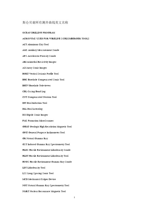
斯仑贝谢所有测井曲线英文名称OCEAN DRILLING PROGRAMACRONYMS USED FOR WIRELINE SCHLUMBERGER TOOLS ACT Aluminum Clay ToolAMS Auxiliary Measurement SondeAPS Accelerator Porosity SondeARI Azimuthal Resistivity ImagerASI Array Sonic ImagerBGKT Vertical Seismic Profile ToolBHC Borehole Compensated Sonic ToolBHTV Borehole TeleviewerCBL Casing Bond LogCNT Compensated Neutron ToolDIT Dual Induction ToolDLL Dual LaterologDSI Dipole Sonic ImagerFMS Formation MicroScannerGHMT Geologic High Resolution Magnetic ToolGPIT General Purpose Inclinometer ToolGR Natural Gamma RayGST Induced Gamma Ray Spectrometry ToolHLDS Hostile Environment Lithodensity SondeHLDT Hostile Environment Lithodensity ToolHNGS Hostile Environment Gamma Ray SondeLDT Lithodensity ToolLSS Long Spacing Sonic ToolMCD Mechanical Caliper DeviceNGT Natural Gamma Ray Spectrometry ToolQSST Inline Checkshot ToolSDT Digital Sonic ToolSGT Scintillation Gamma Ray ToolSUMT Susceptibility Magnetic ToolUBI Ultrasonic Borehole ImagerVSI Vertical Seismic ImagerWST Well Seismic ToolWST-3 3-Components Well Seismic ToolOCEAN DRILLING PROGRAMACRONYMS USED FOR LWD SCHLUMBERGER TOOLSADN Azimuthal Density-NeutronCDN Compensated Density-NeutronCDR Compensated Dual ResistivityISONIC Ideal Sonic-While-DrillingNMR Nuclear Magnetic ResonanceRAB Resistivity-at-the-BitOCEAN DRILLING PROGRAMACRONYMS USED FOR NON-SCHLUMBERGER SPECIALTY TOOLS MCS Multichannel Sonic ToolMGT Multisensor Gamma ToolSST Shear Sonic ToolTAP Temperature-Acceleration-Pressure ToolTLT Temperature Logging ToolOCEAN DRILLING PROGRAMACRONYMS AND UNITS USED FOR WIRELINE SCHLUMBERGER LOGS AFEC APS Far Detector Counts (cps)ANEC APS Near Detector Counts (cps)AX Acceleration X Axis (ft/s2)AY Acceleration Y Axis (ft/s2)AZIM Constant Azimuth for Deviation Correction (deg)APLC APS Near/Array Limestone Porosity Corrected (%)C1 FMS Caliper 1 (in)C2 FMS Caliper 2 (in)CALI Caliper (in)CFEC Corrected Far Epithermal Counts (cps)CFTC Corrected Far Thermal Counts (cps)CGR Computed (Th+K) Gamma Ray (API units)CHR2 Peak Coherence, Receiver Array, Upper DipoleCHRP Compressional Peak Coherence, Receiver Array, P&SCHRS Shear Peak Coherence, Receiver Array, P&SCHTP Compressional Peak Coherence, Transmitter Array, P&SCHTS Shear Peak Coherence, Transmitter Array, P&SCNEC Corrected Near Epithermal Counts (cps)CNTC Corrected Near Thermal Counts (cps)CS Cable Speed (m/hr)CVEL Compressional Velocity (km/s)DATN Discriminated Attenuation (db/m)DBI Discriminated Bond IndexDEVI Hole Deviation (degrees)DF Drilling Force (lbf)DIFF Difference Between MEAN and MEDIAN in Delta-Time Proc. (microsec/ft) DRH HLDS Bulk Density Correction (g/cm3)DRHO Bulk Density Correction (g/cm3)DT Short Spacing Delta-Time (10'-8' spacing; microsec/ft)DT1 Delta-Time Shear, Lower Dipole (microsec/ft)DT2 Delta-Time Shear, Upper Dipole (microsec/ft)DT4P Delta- Time Compressional, P&S (microsec/ft)DT4S Delta- Time Shear, P&S (microsec/ft))DT2R Delta- Time Shear, Receiver Array, Upper Dipole (microsec/ft)DT1T Delta-Time Shear, Transmitter Array, Lower Dipole (microsec/ft)DT2T Delta-Time Shear, Transmitter Array, Upper Dipole (microsec/ft) DTCO Delta- Time Compressional (microsec/ft)DTL Long Spacing Delta-Time (12'-10' spacing; microsec/ft)DTLF Long Spacing Delta-Time (12'-10' spacing; microsec/ft)DTLN Short Spacing Delta-Time (10'-8' spacing; microsec/ftDTRP Delta-Time Compressional, Receiver Array, P&S (microsec/ft) DTRS Delta-Time Shear, Receiver Array, P&S (microsec/ft)DTSM Delta-Time Shear (microsec/ft)DTST Delta-Time Stoneley (microsec/ft)DTTP Delta-Time Compressional, Transmitter Array, P&S (microsec/ft) DTTS Delta-Time Shear, Transmitter Array, P&S (microsec/ft)ECGR Environmentally Corrected Gamma Ray (API units)EHGR Environmentally Corrected High Resolution Gamma Ray (API units) ENPH Epithermal Neutron Porosity (%)ENRA Epithermal Neutron RatioETIM Elapsed Time (sec)FINC Magnetic Field Inclination (degrees)FNOR Magnetic Field Total Moment (oersted)FX Magnetic Field on X Axis (oersted)FY Magnetic Field on Y Axis (oersted)FZ Magnetic Field on Z Axis (oersted)GR Natural Gamma Ray (API units)HALC High Res. Near/Array Limestone Porosity Corrected (%)HAZI Hole Azimuth (degrees)HBDC High Res. Bulk Density Correction (g/cm3)HBHK HNGS Borehole Potassium (%)HCFT High Resolution Corrected Far Thermal Counts (cps)HCNT High Resolution Corrected Near Thermal Counts (cps)HDEB High Res. Enhanced Bulk Density (g/cm3)HDRH High Resolution Density Correction (g/cm3)HFEC High Res. Far Detector Counts (cps)HFK HNGS Formation Potassium (%)HFLC High Res. Near/Far Limestone Porosity Corrected (%)HEGR Environmentally Corrected High Resolution Natural Gamma Ray (API units) HGR High Resolution Natural Gamma Ray (API units)HLCA High Res. Caliper (inHLEF High Res. Long-spaced Photoelectric Effect (barns/e-)HNEC High Res. Near Detector Counts (cps)HNPO High Resolution Enhanced Thermal Nutron Porosity (%)HNRH High Resolution Bulk Density (g/cm3)HPEF High Resolution Photoelectric Effect (barns/e-)HRHO High Resolution Bulk Density (g/cm3)HROM High Res. Corrected Bulk Density (g/cm3)HSGR HNGS Standard (total) Gamma Ray (API units)HSIG High Res. Formation Capture Cross Section (capture units)HSTO High Res. Computed Standoff (in)HTHO HNGS Thorium (ppm)HTNP High Resolution Thermal Neutron Porosity (%)HURA HNGS Uranium (ppm)IDPH Phasor Deep Induction (ohmm)IIR Iron Indicator Ratio [CFE/(CCA+CSI)]ILD Deep Resistivity (ohmm)ILM Medium Resistivity (ohmm)IMPH Phasor Medium Induction (ohmm)ITT Integrated Transit Time (s)LCAL HLDS Caliper (in)LLD Laterolog Deep (ohmm)LLS Laterolog Shallow (ohmm)LTT1 Transit Time (10'; microsec)LTT2 Transit Time (8'; microsec)LTT3 Transit Time (12'; microsec)LTT4 Transit Time (10'; microsec)MAGB Earth's Magnetic Field (nTes)MAGC Earth Conductivity (ppm)MAGS Magnetic Susceptibility (ppm)MEDIAN Median Delta-T Recomputed (microsec/ft) MEAN Mean Delta-T Recomputed (microsec/ft) NATN Near Pseudo-Attenuation (db/m)NMST Magnetometer Temperature (degC)NMSV Magnetometer Signal Level (V)NPHI Neutron Porosity (%)NRHB LDS Bulk Density (g/cm3)P1AZ Pad 1 Azimuth (degrees)PEF Photoelectric Effect (barns/e-)PEFL LDS Long-spaced Photoelectric Effect (barns/e-) PIR Porosity Indicator Ratio [CHY/(CCA+CSI)]POTA Potassium (%)RB Pad 1 Relative Bearing (degrees)RHL LDS Long-spaced Bulk Density (g/cm3)RHOB Bulk Density (g/cm3)RHOM HLDS Corrected Bulk Density (g/cm3)RMGS Low Resolution Susceptibility (ppm)SFLU Spherically Focused Log (ohmm)SGR Total Gamma Ray (API units)SIGF APS Formation Capture Cross Section (capture units) SP Spontaneous Potential (mV)STOF APS Computed Standoff (in)SURT Receiver Coil Temperature (degC)SVEL Shear Velocity (km/s)SXRT NMRS differential Temperature (degC)TENS Tension (lb)THOR Thorium (ppm)TNRA Thermal Neutron RatioTT1 Transit Time (10' spacing; microsec)TT2 Transit Time (8' spacing; microsec)TT3 Transit Time (12' spacing; microsec)TT4 Transit Time (10' spacing; microsec)URAN Uranium (ppm)V4P Compressional Velocity, from DT4P (P&S; km/s)V4S Shear Velocity, from DT4S (P&S; km/s)VELP Compressional Velocity (processed from waveforms; km/s)VELS Shear Velocity (processed from waveforms; km/s)VP1 Compressional Velocity, from DT, DTLN, or MEAN (km/s)VP2 Compressional Velocity, from DTL, DTLF, or MEDIAN (km/s)VCO Compressional Velocity, from DTCO (km/s)VS Shear Velocity, from DTSM (km/s)VST Stonely Velocity, from DTST km/s)VS1 Shear Velocity, from DT1 (Lower Dipole; km/s)VS2 Shear Velocity, from DT2 (Upper Dipole; km/s)VRP Compressional Velocity, from DTRP (Receiver Array, P&S; km/s) VRS Shear Velocity, from DTRS (Receiver Array, P&S; km/s)VS1R Shear Velocity, from DT1R (Receiver Array, Lower Dipole; km/s) VS2R Shear Velocity, from DT2R (Receiver Array, Upper Dipole; km/s) VS1T Shear Velocity, from DT1T (Transmitter Array, Lower Dipole; km/s) VS2T Shear Velocity, from DT2T (Transmitter Array, Upper Dipole; km/s) VTP Compressional Velocity, from DTTP (Transmitter Array, P&S; km/s)VTS Shear Velocity, from DTTS (Transmitter Array, P&S; km/s)#POINTS Number of Transmitter-Receiver Pairs Used in Sonic ProcessingW1NG NGT Window 1 counts (cps)W2NG NGT Window 2 counts (cps)W3NG NGT Window 3 counts (cps)W4NG NGT Window 4 counts (cps)W5NG NGT Window 5 counts (cps)OCEAN DRILLING PROGRAMACRONYMS AND UNITS USED FOR LWD SCHLUMBERGER LOGS AT1F Attenuation Resistivity (1 ft resolution; ohmm)AT2F Attenuation Resistivity (2 ft resolution; ohmm)AT3F Attenuation Resistivity (3 ft resolution; ohmm)AT4F Attenuation Resistivity (4 ft resolution; ohmm)AT5F Attenuation Resistivity (5 ft resolution; ohmm)ATR Attenuation Resistivity (deep; ohmm)BFV Bound Fluid Volume (%)B2TM RAB Medium Resistivity Time after Bit (s)B3TM RAB Deep Resistivity Time after Bit (s)BDAV Deep Resistivity Average (ohmm)BMAV Medium Resistivity Average (ohmm)BSAV Shallow Resistivity Average (ohmm)CGR Computed (Th+K) Gamma Ray (API units)DCAL Differential Caliper (in)DROR Correction for CDN rotational density (g/cm3).DRRT Correction for ADN rotational density (g/cm3).DTAB AND or CDN Density Time after Bit (hr)FFV Free Fluid Volume (%)GR Gamma Ray (API Units)GR7 Sum Gamma Ray Windows GRW7+GRW8+GRW9-Equivalent to Wireline NGT window 5 (cps)GRW3 Gamma Ray Window 3 counts (cps)-Equivalent to Wireline NGT window 1GRW4 Gamma Ray Window 4 counts (cps)-Equivalent to Wireline NGT window 2 GRW5 Gamma Ray Window 5 counts (cps)-Equivalent to Wireline NGT window 3 GRW6 Gamma Ray Window 6 counts (cps)-Equivalent to Wireline NGT window 4 GRW7 Gamma Ray Window 7 counts (cps)GRW8 Gamma Ray Window 8 counts (cps)GRW9 Gamma Ray Window 9 counts (cps)GTIM CDR Gamma Ray Time after Bit (s)GRTK RAB Gamma Ray Time after Bit (s)HEF1 Far He Bank 1 counts (cps)HEF2 Far He Bank 2 counts (cps)HEF3 Far He Bank 3 counts (cps)HEF4 Far He Bank 4 counts (cps)HEN1 Near He Bank 1 counts (cps)HEN2 Near He Bank 2 counts (cps)HEN3 Near He Bank 3 counts (cps)HEN4 Near He Bank 4 counts (cps)MRP Magnetic Resonance PorosityNTAB ADN or CDN Neutron Time after Bit (hr)PEF Photoelectric Effect (barns/e-)POTA Potassium (%) ROPE Rate of Penetration (ft/hr)PS1F Phase Shift Resistivity (1 ft resolution; ohmm)PS2F Phase Shift Resistivity (2 ft resolution; ohmm)PS3F Phase Shift Resistivity (3 ft resolution; ohmm)PS4F Phase Shift Resistivity (4 ft resolution; ohmm)PS5F Phase Shift Resistivity (5 ft resolution; ohmm)PSR Phase Shift Resistivity (shallow; ohmm)RBIT Bit Resistivity (ohmm)RBTM RAB Resistivity Time After Bit (s)RING Ring Resistivity (ohmm)ROMT Max. Density Total (g/cm3) from rotational processingROP Rate of Penetration (m/hr)ROP1 Rate of Penetration, average over last 1 ft (m/hr). ROP5 Rate of Penetration, average over last 5 ft (m/hr) ROPE Rate of Penetration, averaged over last 5 ft (ft/hr) RPM RAB Tool Rotation Speed (rpm)RTIM CDR or RAB Resistivity Time after Bit (hr)SGR Total Gamma Ray (API units)T2 T2 Distribution (%)T2LM T2 Logarithmic Mean (ms)THOR Thorium (ppm)TNPH Thermal Neutron Porosity (%)TNRA Thermal RatioURAN Uranium (ppm)OCEAN DRILLING PROGRAMADDITIONAL ACRONYMS AND UNITS(PROCESSED LOGS FROM GEOCHEMICAL TOOL STRING)AL2O3 Computed Al2O3 (dry weight %)AL2O3MIN Computed Al2O3 Standard Deviation (dry weight %) AL2O3MAX Computed Al2O3 Standard Deviation (dry weight %) CAO Computed CaO (dry weight %)CAOMIN Computed CaO Standard Deviation (dry weight %) CAOMAX Computed CaO Standard Deviation (dry weight %) CACO3 Computed CaCO3 (dry weight %)CACO3MIN Computed CaCO3 Standard Deviation (dry weight %) CACO3MAX Computed CaCO3 Standard Deviation (dry weight %) CCA Calcium Yield (decimal fraction)CCHL Chlorine Yield (decimal fraction)CFE Iron Yield (decimal fraction)CGD Gadolinium Yield (decimal fraction)CHY Hydrogen Yield (decimal fraction)CK Potassium Yield (decimal fraction)CSI Silicon Yield (decimal fraction)CSIG Capture Cross Section (capture units)CSUL Sulfur Yield (decimal fraction)CTB Background Yield (decimal fraction)CTI Titanium Yield (decimal fraction)FACT Quality Control CurveFEO Computed FeO (dry weight %)FEOMIN Computed FeO Standard Deviation (dry weight %) FEOMAX Computed FeO Standard Deviation (dry weight %) FEO* Computed FeO* (dry weight %)FEO*MIN Computed FeO* Standard Deviation (dry weight %) FEO*MAX Computed FeO* Standard Deviation (dry weight %) FE2O3 Computed Fe2O3 (dry weight %)FE2O3MIN Computed Fe2O3 Standard Deviation (dry weight %) FE2O3MAX Computed Fe2O3 Standard Deviation (dry weight %) GD Computed Gadolinium (dry weight %)GDMIN Computed Gadolinium Standard Deviation (dry weight %) GDMAX Computed Gadolinium Standard Deviation (dry weight %) K2O Computed K2O (dry weight %)K2OMIN Computed K2O Standard Deviation (dry weight %)K2OMAX Computed K2O Standard Deviation (dry weight %) MGO Computed MgO (dry weight %)MGOMIN Computed MgO Standard Deviation (dry weight %) MGOMAX Computed MgO Standard Deviation (dry weight %)S Computed Sulfur (dry weight %)SMIN Computed Sulfur Standard Deviation (dry weight %) SMAX Computed Sulfur Standard Deviation (dry weight %)SIO2 Computed SiO2 (dry weight %)SIO2MIN Computed SiO2 Standard Deviation (dry weight %) SIO2MAX Computed SiO2 Standard Deviation (dry weight %) THORMIN Computed Thorium Standard Deviation (ppm) THORMAX Computed Thorium Standard Deviation (ppm) TIO2 Computed TiO2 (dry weight %)TIO2MIN Computed TiO2 Standard Deviation (dry weight %) TIO2MAX Computed TiO2 Standard Deviation (dry weight %) URANMIN Computed Uranium Standard Deviation (ppm) URANMAX Computed Uranium Standard Deviation (ppm) VARCA Variable CaCO3/CaO calcium carbonate/oxide factor。

第28卷㊀第2期2023年4月㊀哈尔滨理工大学学报JOURNAL OF HARBIN UNIVERSITY OF SCIENCE AND TECHNOLOGY㊀Vol.28No.2Apr.2023㊀㊀㊀㊀㊀㊀㊀㊀㊀㊀架空输电线路弧垂及覆冰的在线监测杨小龙,㊀袁翰青,㊀孙辰军,㊀马㊀超,㊀李㊀静(国网河北省电力有限公司信息通信分公司,石家庄050000)摘㊀要:为实现架空输电线路在线覆冰及舞动监测,提出了一种基于分布式相敏光时域反射计(Φ-OTDR )架空输电线路在线监测方法㊂文章通过建立了输电线路的数学模型,理论分析得到导线的弧垂㊁舞动频率等参数计算公式;其次提出了基于Φ-OTDR 分析方法,并对其监测原理进行了分析㊂通过搭建架空线在线监测模型,分别开展架空线舞动试验及覆冰试验,分析得到了架空输电线路的动态应变特性,验证了基于Φ-OTDR 的输电线路状态在线监测方案㊂试验结果表明,在厘米尺度上,弧垂估计误差小于5.8%,在亚毫米尺度上,冰厚估计误差不大于10.84%,可准确描述了输电线路状态,为输电线路故障预警提供了有力支持㊂关键词:分布式光纤传感器;在线监测;架空输电线路;Φ-OTDR DOI :10.15938/j.jhust.2023.02.012中图分类号:TM726.3文献标志码:A文章编号:1007-2683(2023)02-0099-09On-line Monitoring of Sag and Icing of Overhead Transmission LinesYANG Xiaolong,㊀YUAN Hanqing,㊀SUN Chenjun,㊀MA Chao,㊀LI Jing(Information and Communication Branch of State Grid Hebei Electric Power Co.,Ltd.,Shijiazhuang,050000)Abstract :In order to realize on-line icing and galloping monitoring of overhead transmission lines,an on-line monitoring method for overhead transmission lines based on phase-sensitive optical time domain reflectometry (Φ-OTDR)is proposed.In this paper,by establishing mathematical models of transmission line,the calculation formulas of conductor sag,galloping frequency and other parameters are obtained through theoretical analysis.Secondly,by building the overhead line online monitoring model,the overheadline galloping test and the icing test are proposed respectively,and the leakage principle is analyzed.The dynamic acquisition characteristics of overhead transmission lines are analyzed,and the online status monitoring scheme of transmission lines based on Φ-OTDR is verified.The test results show that the estimation error of sag is less than 5.8%on centimeter scale,and the estimation error of ice thickness is no more than 10.84%on sub-millimeter scale,which gives an accurate description of transmission line status andprovides strong support for early warning of transmission line failures.Keywords :distributed optical fiber sensor;online monitoring;overhead transmission line;phase-sensitive OTDR㊀㊀㊀㊀㊀㊀㊀㊀㊀㊀㊀㊀㊀㊀㊀㊀㊀㊀㊀㊀㊀㊀㊀㊀㊀㊀㊀㊀㊀㊀㊀㊀㊀㊀㊀㊀㊀㊀㊀㊀㊀㊀㊀㊀㊀㊀㊀㊀㊀㊀㊀㊀㊀㊀㊀㊀㊀㊀㊀㊀㊀㊀㊀㊀㊀㊀㊀㊀㊀㊀㊀㊀㊀㊀㊀㊀㊀㊀㊀㊀㊀㊀㊀㊀㊀㊀㊀㊀㊀㊀㊀㊀㊀㊀㊀㊀㊀㊀㊀㊀㊀㊀㊀㊀㊀㊀收稿日期:2021-10-14基金项目:科技部科技创新重大项目(2020AAA0107500).作者简介:袁翰青(1973 ),男,硕士,高级工程师;孙辰军(1981 ),男,硕士,高级工程师.通信作者:杨小龙(1989 ),男,硕士,高级工程师,E-mail:277135930@.0㊀引㊀言由于我国东西部资源与消费的严重不均,通过高压远距离传输电能,实现资源在国家内部的优化配置成为了必然选择㊂当前,国内多个区域架空输电线路经常受到覆冰和舞动的威胁[1-3]㊂输电线路的载荷和迎风面积通常由于结冰而增加,可能导致架空线路舞动,进而导致断线㊁倒塔㊁闪络等事故,造成巨大的经济损失[2,4,5]㊂因此有必要采用可靠有效的检测方法,及时㊁准确地获取输电线路的覆冰状态㊂目前,输电线路的在线监测主要通过点传感器或图像监测实现[6-9]㊂大多数点传感器是电传感器,通常都存在非线性㊁零点漂移和强电磁环境耐受差等缺点[10-11]㊂此外,这些传感器的安装,包括电源和数据传输网络布设实施步骤复杂且费用较高㊂光纤传感器(optical fiber sensors,OFSs)是一种以光波为载体㊁光纤为传感介质的传感器,随着光纤通信技术的发展,应用已愈来愈广泛㊂OFSs具有一系列独特的优点,如测量精度高㊁鲁棒性好和绝缘性能高㊂基于OFS的传输线监测始于1997年,其中光纤布拉格光栅(fiber bragg gratings,FBG)可用于测量相邻两个城镇之间输电线路的应变[12]㊂但由于FBG制造和部件成本较高,通常比同类电子产品贵一到两个数量级㊂此外,与电子传感器一样,FBG 属于单点传感器,只能提供较低的传感器分布密度㊂此传感器必须采用额外传输线路连接到输电线路,这会降低传输线的稳定性㊂与光纤光栅不同,分布式光纤传感器(distribu-ted optical fiber sensors,DOFSs)依靠一整套光学系统与光纤一起实现对物理电气参数进行采集和空间解调,可以取代成千上万的点传感器㊂因此,DOFSs 可以用来监测目标的整体行为,而不是从几个测量点进行外推㊂电力传输系统中的通信主要基于光缆,同时光纤复合架空地线(optical fiber composite overhead ground wire,OPGW)得到了广泛的应用㊂通过DOFSs,OPGW网络可以构成在线监测的传感网络㊂目前基于DOFSs的输电线路覆冰在线监测主要通过布里渊光时域反射计(BOTDR)监测输电线路的应变变化来实现[13-16]㊂虽然研究人员已经证明了该方案的可行性,但仍有一些不足之处㊂首先,光纤一般有0.6%~0.7%长度的尾纤,其中填充的润滑脂降低了光纤附着力[7,12],使得架空线的应力很难作用在光纤上㊂因此,只有当外部张力大于阈值时,才能测量架空线的应变㊂此外,BOTDR 的单个采集周期通常为几十分钟,由于舞动,架空线的应变将会不断变化,这可能导致测量结果不准确㊂这些缺点共同带来应力测量的不确定性,进而导致测量结果的置信度较低㊂近年来,具有高灵敏度实时测量能力的相敏光时域反射计(Φ-OTDR)引起了众多研究人员的兴趣[6-10,17-21]㊂Φ-OTDR具有响应速度快㊁机械振动灵敏度高等优点,适于输电线路的在线监测㊂2019年,有研究人员使用Φ-OTDR监测传输线的舞动频率,并将结果与FBG的结果进行比较,但他们并未对这些参数代表的意义以及如何利用它们进行进一步解释或分析[22]㊂本文基于输电线路数学模型,提出了基于Φ-OTDR的在线监测的分析方法;搭建架空线路弧垂㊁覆冰监测平台,通过试验证明Φ-OTDR的测量结果(包括弧垂㊁舞动㊁覆冰)的准确性㊂1㊀在线监测原理分析1.1㊀输电线路的力学特性分析在分析输电线路力学特性时,建立一个包含导线㊁减震器㊁绝缘子串和杆塔的全套计算模型是非常复杂和困难的㊂相对于架空线路而言,塔架可视为刚性固定,因此输电线路模型在分析时可简化为无刚度和无阻尼的导线,导线两端的边界可认为是固定㊂图1㊀无刚度和阻尼的导线Fig.1㊀A wire with no stiffness and no damping如图1所示,L为导线的长度;l为跨度长度;h 为从导线弧垂的最低点到两固定点连接线的垂直距离;T0为导线的初始水平张力㊂那么导线长度㊁跨距和弧垂之间的关系可以表示为[20]L=l+8h23l(1)当覆冰或落冰时,L将相应地改变ΔL,此时弧垂可以表示为hᶄ=3l8ΔL+h20(2)其中:h0为初始弧垂;hᶄ为L变化后的弧垂㊂故只要获得ΔL,就可以计算得到hᶄ㊂导线振动的固有频率是其固有特性之一,可表示为[21]f k=k2l T0m(3)其中:k为振动阶数;f k为k阶震动的频率;m为单位长度导线的质量㊂用裸导线的振动频率除以覆冰001哈㊀尔㊀滨㊀理㊀工㊀大㊀学㊀学㊀报㊀㊀㊀㊀㊀㊀㊀㊀㊀㊀第28卷㊀导线的振动频率:f icef 0=m 0m 0+m ice(4)m ice =ρice d (d -2r 0)(5)式中:m 0为导线单位长度的初始质量;m ice 为每单位长度导线的覆冰质量;r 0为导线的初始半径;d 为冰厚度;ρice 为冰的密度(0.92g /cm 3),由于覆冰厚度仅与导线振动频率比的变化有关㊂将式(5)代入式(4),振动频率与冰厚度之间的关系可以表示为d =m 0(f 20-f 2ice )πρice f 2ice+r 20-r 0(6)因此,通过对输电线路振动频率的检测,可以得到覆冰厚度㊂1.2㊀Φ-OTDR 监测原理分析Φ-OTDR 利用窄线宽激光产生高相干光脉冲,在传感光纤上获得相对稳定的瑞利背向散射(Ray-leigh backscatter,RBS)相位分布㊂在没有外界干扰和不考虑激光频率漂移的情况下,传感光纤任意截面上的RBS相位都是稳定的㊂当振动信号作用于传感光纤时,传感光纤的形状将会因振动信号而产生受力形变,光纤的折射率㊁长度和纤芯直径都会发生变化,从而导致RBS 的相位变化㊂因此,可通过测量RBS 相位差的变化来解调该部位光纤的振动信号㊂图2㊀振动引起RBS 相变Fig.2㊀Vibration causes the phase change of RBS如图2所示,r 1和r 2分别为传感光纤扰动区前后的散射中心;S 0是r 1和r 2之间初始光纤的长度㊂当相干光脉冲在传感光纤中传播时,入射光将在每个散射中心激发相干RBS㊂在仅考虑传感光纤轴向应变引起的相变时,r 1和r 2处RBS 的简化表达式可写成[23]:E r 1=E 1cos(ωt +φ1)(7)E r 2=E 2cos ωt +φ1+4πnλ(S 0+ΔS )()(8)其中:E 1和E 2为RBS 的振幅;ω为入射光角频率;φ1为初始相位;n 为光纤芯的折射率;λ为入射光的波长;ΔS 为振动引起的长度变化㊂由此,r 1和r 2之间的相位差为[24]Δφ=4πn λS 0+4πnλΔS =φS 0+Δφυ(9)式中:φS 0为初始光纤长度引入的相位差,它决定了相位差曲线的初始位置,在稳定环境下通常为常数;Δφυ为振动引入的相位差,决定相位差曲线的形状㊂因此,可通过RBS 信号检测和数据处理,解调相位变化以及光纤长度变化㊂由于光纤长度的变化与振动幅度呈线性关系,从而实现振动的精确测量㊂1.3㊀基于Φ-OTDR 的输电线路在线监测假设图2中的导线为OPGW,两个端点分别为r 1和r 2,可通过Φ-OTDR 获得导线的长度变化㊂首先,假设OPGW 的负载在无振动的情况下发生变化,L 也会相应变化,其该变量ΔL 可以表述为[25]ΔL =S ᶄ0-S 0=λ4πn(φᶄS 0-φS 0)(10)式中:S ᶄ0为荷载变化后的光纤长度;φᶄS 0为光纤长度变化后相位差曲线的水平位置㊂需要指出的是,尽管由于环境不稳定,φS 0可能随时间而缓慢变化,冻雨或冰降引起的输电线路负荷变化通常是快速或突然的,所以φS 0对计算影响不大㊂因此,通过观察相位差曲线的水平位置变化,弧垂的计算表达式为h ᶄ=3λl32πn(φᶄS 0-φS 0)+h 20(11)然后假设风导致架空线舞动,导线负载保持不变,L 也会相应变化,ΔL 可以表述为ΔL =ΔS =λ4πn Δφυ(12)平衡状态下最低位置弧垂变化可表示为[25]G =3λl32πnΔφυ+h 20-h 0(13)这里,弧垂的变化反映为振幅变化,也可以相应地获得振动频率㊂由此,可以通过将荷载变化前后的固有频率代入式(6)来计算冰厚度㊂应该注意的是根据式(3),f 与l ㊁T 0和m 相关,因此不同跨度中f 0也不一致㊂于是需要根据不同跨度的实际测量结果校准f ㊂此外,根据式(3)和式(4),当冰厚度相同时,振动阶数越高,f 0和f ice 之间的差异越大㊂由此可知,高阶振动对输电线路的负荷变化更为敏感㊂101第2期杨小龙等:架空输电线路弧垂及覆冰的在线监测2㊀试验研究2.1㊀试验平台搭建本文搭建了演示试验系统,其硬件设置示意图如图3所示㊂所使用的Φ-OTDR 设备为日本光纳株式社生产,型号为NBX -S300,设备采样率为4kHz,空间分辨率为0.1m,测量距离可达100m㊂设计的铝合金框架用于悬挂钢绞线,考虑后续覆冰及舞动试验施加的激励方式,本文在实验室内开展模拟试验时以钢丝绳替代导线,分析覆冰和舞动的情况㊂导线在固定滑轮上缠绕数米以此作为固定方式,试验布置时设定两个固定滑轮之间的距离即跨度为30m,将0.9mm 的光纤紧密固定在导线上㊂将一根100g 的绳子悬挂在导线的中心(即跨度的中间位置),通过切割绳子释放悬挂在导线上的重量来激发导线振动㊂利用H 1减去H 2获得导线的初始弧垂,其中H 1是固定点的高度,H 2是导线最低点的高度,可随冰厚度的变化而变化㊂本文所使用的导线(即上文提到的钢丝绳)直径和单位长度质量分别为1.5mm 和46.4g /m㊂由于很难实现导线覆冰均匀且各处位置厚度一致,所以本文用橡皮泥来替代实际的冰,也可达到导线荷载增加的效果㊂在开展覆冰试验时,冰的厚度逐渐从0.25mm 增加至为1.25mm,梯度为0.25mm,冰的质量可以根据式(5)进行计算㊂图3㊀覆冰舞动模拟装置原理图Fig.3㊀Schematic diagram of the device forsimulating icing and galloping2.2㊀试验结果分析2.2.1㊀舞动试验图4(a)为振动的功率谱密度(power spectraldensity,PSD),可以看出主振动频率约为1.3Hz,中间振动强度最大,两侧减小㊂有9个区域受到悬挂重物重量下降的影响,选择中间7个区域分析振动变化,其振动情况一致,如图4(b)所示㊂然后,沿导线方向进行积分,可以获得整个振动过程的相位变化,如图4(c)所示㊂分析图4(c),由于悬挂物重量的下降,将使得悬挂中心位置产生46000rad 的振动,且振动强度呈指数衰减并逐渐趋于稳定㊂图4㊀导线舞动试验结果Fig.4㊀Wire galloping test result首先对弧垂进行评估,依次卸下5个悬挂在线路中间的重量为10g 的橡皮块㊂图5(a)为导线悬挂部分随橡皮块卸下的相位变化,初始值为0rad,随着悬挂重物重量的减轻,相位逐渐向y 轴负方向移动,这意味着悬挂导线的长度变短,弧垂也应相应减小㊂图5(b)为用软尺测量的实际弧垂,以及校正201哈㊀尔㊀滨㊀理㊀工㊀大㊀学㊀学㊀报㊀㊀㊀㊀㊀㊀㊀㊀㊀㊀第28卷㊀前后的估计弧垂㊂弧垂测量值和估计值的趋势一致,由于两者绝对误差几乎为常数,故实际值和未经校正的估计值之间的相对误差随着弧垂的减小而增大㊂可以看出,实际值和估计值之间的误差单调,且估计值均大于实际值,如图5(c)所示㊂根据式(11)和式(9),如果h ᶄ高于实际值,则S 0-S ᶄ0小于其理论值,误差最有可能是光纤与导线的固定松动而引起的㊂由图5(b)得出,实际值和未经校正的估计值之间的平均差为0.0158m,将该差值和初始弧垂(0.458m )代入式(1),计算出的额外长度为0.0016m㊂经校正后,实际值与估计值之间的相对误差减小了一个数量级以上,均小于5.8%㊂图5㊀弧垂测量结果分析Fig.5㊀Analysis of sag measurement results进一步分析光纤固定松动引起的额外长度变化,在式(2)中引入了误差项ΔL ,有无额外长度的弧垂估计表示如下:h 1=3l8ΔL +h 20(14)h ᶄ1=3l8(ΔL +ΔL ᶄ)+h 20(15)相对误差可以表示为h ᶄ1-h 1h 1=1+ΔLΔL +83lh 2-1(15)220kV 输电网络的跨度通常为100m,假设l =400m,h 0=10m,h 1从10.5m 增加到12.5m,间隔为0.5m,ΔL 的取值范围为0.1ɢ~0.3ɢ,接着计算相对误差,如图5(d)所示㊂可以看出,在引入实际刻度参数后,虽然额外长度的比例增加,但相对误差小于10%,并且随着弧垂的增加而减小㊂显然,由于模拟设备与实际情况之间存在一定差异,引起误差放大㊂对相变曲线上进行高通滤波,截止频率设定为0.5Hz,以获得Δφυ,可根据式(13)计算最低点的位移㊂为了评估计算结果的准确性,在导线的最低点布置了MEMS 加速度计作为对比,其分辨率为6.1ˑ10-5g,传感范围为ʃ16g㊂将加速度器的结果进行两次积分,可以得到最低点的位移信息㊂如图6(a)所示,加速度器和Φ-OTDR 获得的位移信息基本一致,这证明等式(13)给出的转换关系是有效的㊂图6(b)给出了振动的PSD 图,可得导线固有振动频率的值,证明了加速度器和Φ-OTDR 结果的一致性㊂301第2期杨小龙等:架空输电线路弧垂及覆冰的在线监测因此,在已知初始垂度的情况下,Φ-OTDR 可以检测导线的位移㊂图6㊀振动频谱分析Fig.6㊀Vibration spectrum analysis2.2.2㊀覆冰试验图7为覆冰厚度变化后悬挂部分导线的相位变化,它不仅体现了振动激励的一致性,还描述了导线振动固有频率的变化㊂随着振动的不断变化,由于共振,振动能量逐渐集中在导线的固有频率上㊂图7㊀不同冰厚下的相变Fig.7㊀Phase change under different ice thickness通过比较振动PSD,可以进一步分析振动频率与冰厚之间的关系㊂图8(a)为不同冰厚下的振动PSD,可以看出振动具有多个频率分量㊂根据式(3),一次谐波和二次谐波之间的频率间隔应与二次谐波和三次谐波之间的间隔相同,但观察图8(a)明显与理论不符,将图8(a)局部放大为图8(b)㊁(c)和(d)㊂很明显,随着冰厚度的增加,振动频率向低频漂移,其关系如图8(e)所示㊂高次谐波的频移对冰厚的变化更为敏感,冰厚度与f /f 0之间的关系如图8(f)所示㊂401哈㊀尔㊀滨㊀理㊀工㊀大㊀学㊀学㊀报㊀㊀㊀㊀㊀㊀㊀㊀㊀㊀第28卷㊀图8㊀覆冰试验结果分析Fig.8㊀Analysis of icing test results㊀㊀根据式(4),f/f0的值仅受导线质量的影响,因此对于不同的f0,比率的变化趋势应该是相同的㊂在图8(f)中,当f0为3.0275Hz和5.0225Hz时,比率变化一致,而当f0为1.34Hz时,斜率显著不同,这表明这组频率不符合等式(3)㊂分析原因,认为这组频率的出现是由铝合金框架的振动引起的㊂一方面,在由导线和铝合金框架组成的振动系统中,铝合金框架在外力作用下可能发生低频弹性变形,振动频率低于由绳索和固定点组成的振动系统㊂另一方面,由于铝合金架质量较大,导线质量变化引起的整体振动频率变化相对较小㊂结果表明,1.34Hz 左右的频率簇出现在低频段,对冰厚的变化不太敏感㊂分析二阶和三阶谐波的变化,根据式(6)可计算预估的覆冰厚度,结果如图9所示㊂估计值与实际值吻合良好,在亚毫米尺度上绝对偏差小于10.84%,这意味着可以线路结冰初始阶段即产生预警信息㊂图9㊀实际与预测的冰厚度Fig.9㊀Actual and estimated ice thickness3㊀结㊀论综上所述,本文建立了输电线路状态的数学模型,通过分析黏附在导线上光纤的相变特性,提出了基于Φ-OTDR的在线监测方案的分析方法,并搭建了演示装置对分析结果进行验证㊂试验结果表明,在厘米尺度上,弧垂的预测误差小于5.8%,在亚毫米尺度上,覆冰厚度的预测误差不大于10.84%㊂因此,本文的研究结果可为输电线路的日常检查和维护提供了有效途径,且具有更低的成本㊁更高的可信度和更早的警告㊂虽然本文已做了较多的工作,然而在工程应用中仍存在一些问题需要解决㊂首先,OPGW中光纤的额外长度将影响弧垂和振动测量,尾纤的存在可能导致弧垂预测偏大和振动位移预测偏小㊂其次,固有频率的选择决定了覆冰厚度预测的准确性㊂对于实际输电线路,振动的激励源通常是强风,除固有频率外,强风还可能引起更多频率分量㊂因此,还需对此方法开展深度研究,从而实现工程应用㊂另外,本文试验研究时考虑的是均匀覆冰,与实际存在一定差别,后续将在覆冰实验室开展试验,验证本文方法工程应用的可行性㊂501第2期杨小龙等:架空输电线路弧垂及覆冰的在线监测参考文献:[1]㊀李海荣.500kV架空输电线路次档距振荡原因与防范策略的分析[J].电工技术,2018(17):120.LI Hairong.Causes Analysis and Prevention Strategies ofSubspan Oscillation of500kV Overhead TransmissionLines[J].Electric Engineering,2018(17):120. [2]㊀刘亮,郝震,崔赟,等.架空线路无覆冰导线舞动的参数共振机理[J].振动工程学报,2018,31(2):308.LIU Liang,HAO Zhen,CUI Yun,et al.Parametric Res-onance Mechanism of Conductor Galloping Without Icingon Overhead Lines[J].Journal of Vibration Engineering,2018,31(2):308.[3]㊀刘文峰,袁翔,傅建宇.架空线路覆冰在线监测模型的研究现状[J].电子测试,2019(14):44.LIU Wenfeng,YUAN Xiang,FU Jianyu.Research Statusof Iced Calculation Models for Overhead Lines[J].Elec-tronic Test,2019(14):44.[4]㊀李党学,李锐.架空输电线路弧垂检测方法综述[J].电力与能源,2019,40(6):664.LI Dangxue,LI Rui.Overview of Sag Detection Methodsfor Overhead Transmission Lines[J].Power&Energy,2019,40(6):664.[5]㊀李清,杨晓辉,刘振声,等.基于灰色聚类分析的输电线路舞动分级预警方案[J].电测与仪表,2020,57(17):45.LI Qing,YANG Xiaohui,LIU Zhensheng,et al.GradedWarning Scheme of Transmission Line Galloping Based onGrey Clustering Analysis[J].Electrical Measurement&Instrumentation,2020,57(17):45.[6]㊀彭波,赵彬,刘彬,等.一种基于超长弹性细杆模型的大截面导线弧垂计算方法[J].电测与仪表,2018,55(4):70.PENG Bo,ZHAO Bin,LIU Bin,et al.A Method for SagCalculation of Conductor with Large Section Based on Su-per Long Thin Elastic Rod Model[J].Electrical Meas-urement&Instrumentation,2018,55(4):70. [7]㊀林金树,吴润发.基于声表面波技术的配电网架空线温度无源无线监测系统[J].电子测量技术,2020,43(13):167.LIN Jinshu,WU Runfa.Passive-wireless TemperatureMonitoring System Based on SAW Technology for Over-head Transmission in Distribution Network[J].Electron-ic Measurement Technology,2020,43(13):167. [8]㊀刘云鹏,田源,步雅楠,等.光纤检测变压器绕组变形的特征提取与聚类分析[J].电测与仪表,2018,55(21):93.LIU Yunpeng,TIAN Yuan,BU Yanan,et al.Feature Ex-traction and Cluster Analysis of Transformer Winding De-formation by Optical Fiber Detection[J].ElectricalMeasurement&Instrumentation,2018,55(21):93.[9]㊀LUO J,HAO Y,YE Q,et al.Development of OpticalFiber Sensors Based on Brillouin Scattering and FBG forOn-line Monitoring in Overhead Transmission Lines[J].Journal of Lightwave Technology,2013,31(10):1559.[10]CHAOXIANG L,HUAJIAN W,WENBO L,et al.ImageProcessing and Recognition Technology for TransmissionLine Icing[J].Electric Power,2014,47(9):132.[11]ZENG X,LUO X,LU J,et al.A Novel Thickness De-tection Method of Ice Covering on Overhead TransmissionLine[J].Energy Procedia,2012,14:1349. [12]OGAWA Y,IWASAKI J,NAKAMURA K.A Multiple-xing LoadMonitoring System of Power Transmission Linesusing Fiber Bragg Grating[C]//Optical Fiber Sensors.Optical Society of America,1997:OThC16. [13]司召鹏,卜泽华,毛邦宁,等.基于相位解调的相位敏感光时域反射计研究[J].激光与光电子学进展,2022,59(11):109.SI Zhaopeng,BU Zehua,MAO Bangning,et al.Review ofResearch on Phase Sensitive Optical Time Domain Reflec-tometer Based on Phase Demodulation[J].Laser&Opto-electronics Progress,2022,59(11):109. [14]钟翔,赵世松,邓华夏,等.基于脉冲调制的Φ-OTDR研究综述[J].红外与激光工程,2020,49(10):193.ZHONG Xiang,ZHAO Shisong,DENG Huaxia,et al.Re-view of Research onΦ-OTDR System Based on PulseModulation[J].Infrared and Laser Engineering,,2020,49(10):193.[15]王敏学,李黎,周达明,等.分布式光纤传感技术在输电线路在线监测的应用研究综述[J].电网技术,2021,45(9):3591.WANG Minxue,LI Li,ZHOU Daming,et al.Overview ofResearch on Application of Distributed Optical FiberSensing Technology in Online Monitoring of TransmissionLines[J].Power System Technology,2021,45(9):3591.[16]马皓钰,王夏霄,马福,等.Φ-OTDR型分布式光纤声波传感器研究进展[J].激光与光电子学进展,2020,57(13):66.MA Haoyu,WANG Xiaxiao,MA Fu,et al.ResearchProgress ofΦ-OTDR Distributed Optical Fiber AcousticWave Sensor[J].Laser&Optoelectronics Progress,2020,57(13):66.[17]袁敬中,潘国兵,谢景海,等.基于多模空间距离权重融合的高压架空输电线舞动监测模块的设计[J].电力系统保护与控制,2020,48(24):173.YUAN Jingzhong,PAN Guobing,XIE Jinghai,et al.601哈㊀尔㊀滨㊀理㊀工㊀大㊀学㊀学㊀报㊀㊀㊀㊀㊀㊀㊀㊀㊀㊀第28卷㊀Design of a Galvanic Monitoring Module for High-voltageOverhead Transmission Lines Based on the Fusion ofMulti-mode Spatial Distance Weights[J].Power SystemProtection and Control,2020,48(24):173. [18]郑高铭,焦新泉,贾兴中.基于基线偏移的加速度积分速度与位移的方法[J].电测与仪表,2021,58(9):142.ZHENG Gaoming,JIAO Xinquan,JIA Xingzhong.Meth-od for Calculating Velocity and Displacement Based onAcceleration of Baseline Offset[J].Electrical Measure-ment&Instrumentation,2021,58(9):142. [19]吴超,王峥,庞振江,等基于φ-OTDR的架空输电线路风振检测系统设计[J].自动化与仪器仪表,2019(9):46.WU Chao,WANG Zheng,PANG Zhenjiang,et al.Designof the Wind-vibration Detection System for Overhead Pow-er Line Based onφ-OTDR[J].Automation&Instrumen-tation,2019(9):46.[20]葛雄,雷雨,侯新文,等.输电线路导线覆冰舞动时力学特性分析[J].江西电力,2019,43(12):33.GE Xiong,LEI Yu,HOU Xinwen,et al.Analysis of Me-chanical Characteristics of Transmission Line Conductorsunder Ice Coating and Galloping[J]Jiangxi Electric Pow-er,2019,43(12):33.[21]谢占山,李忠芳,王少夫.架空线张力与频率关系理论与试验的研究[J].哈尔滨师范大学自然科学学报,2014,30(3):62.XIE Zhanshan,LI Zhongfang,WANG Shaofu.Researchon the Theory and Test of the Relationship Between Over-head Wire Tension and Frequency[J].Natural ScienceJournal of Harbin Normal University,2014,30(3):62.[22]CHAI Q,LUO Y,REN J,et al.Review on Fiber-opticSensing in Health Monitoring of Power Grids[J].OpticalEngineering,2019,58(7):072007.[23]MA G,SHI C,QIN W,et al.A Non-intrusive ElectricalDischarge Localization Method for Gas Insulated LineBased on Phase-sensitive OTDR and Michelson Interfer-ometer[J].IEEE Transactions on Power Delivery,2019,34(4):1324.[24]董向华.基于φ-OTDR技术的海缆扰动监测系统的研究[J].光纤与电缆及其应用技术,2016(3):32.DONG Xianghua.Research on the Submarine Optical Ca-ble Disturbance Monitoring System Based onφ-OTDRTechnology[J].Optical Fiber&Electric Cable and TheirApplications,2016(3):32.[25]杨斌,皋魏,席刚.Φ-OTDR分布式光纤传感系统的关键技术研究[J].光通信研究,2012(4):19.YANG Bin,GAO Wei,XI Gang.Key Technology ofΦ-OTDR-based Distributed Fiber-optical Sensing Systems[J].Study on Optical Communications,2012(4):19.[26]孙毅,赵泰,侯思祖.基于OTDR的光纤在线监测系统实验研究[J].华北电力大学学报,2004(5):78.SUN Yi,ZHAO Tai,HOU Sizu.Experimental of OpticalFiber Monitoring System Based on OTDR[J].Journal ofNorth China Electric Power University,2004(5):78.(编辑:温泽宇)701第2期杨小龙等:架空输电线路弧垂及覆冰的在线监测。

基于HITEMP数据库的分子吸收光谱高精度快速建模方法钱宝健，蔡静*，常海涛，高一凡（航空工业北京长城计量测试技术研究所，北京 100095）摘要：为解决高温环境下分子吸收光谱精确计算的时间复杂性，满足宽光谱测量领域对理论吸收光谱计算的需求，本研究利用Python语言以逐线计算为基础，结合线型函数的简化、线翼截止准则和谱线数据库的优化，建立了基于高温分子吸收参数数据库（High⁃Temperature molecular spectroscopic absorption parameters data⁃base，HITEMP）的分子吸收光谱精确快速计算模型。

以Hartmann⁃Tran线型函数作为吸收光谱标准线型编写部分相关二次速度依赖硬碰撞函数（partially⁃Correlated quadratic⁃Speed⁃Dependent Hard⁃Collision Profile，pCqSDHC），结合复概率函数（Complex Probability Function，CPF）简化模型实现了线型函数的精确快速计算，相较于理论计算模型计算速度提高了20倍。

按照光谱计算残差在10-5量级确定了固定波数截断结合谱线半宽等倍数截断的线翼截止准则。

以阈值线强度10-25 cm-1/(mol∙cm-2)为标准筛选了每100 K温度梯度时的光谱数据，整合得到优化数据库。

在6 500 ~ 8 000 cm-1范围内对水分子的吸收光谱进行计算，并与“”分子气体集成光谱建模网站仿真结果对比，逐线模型的计算误差在10-7量级，优化模型的计算误差在10-5量级，计算速度平均提升25倍。

该模型满足吸收光谱测量中对于理论吸收光谱的高效准确计算，为复杂环境中基于宽调谐、超连续激光吸收光谱的测量研究提供了理论模型基础。

关键词：吸收光谱；HITEMP数据库；线型函数；线翼截止中图分类号：TB9；O433 文献标志码：A 文章编号：1674-5795（2023）05-0039-10Modeling molecular absorption spectra based on the HITEMP databaseQIAN Baojian, CAI Jing*, CHANG Haitao, GAO Yifan(Changcheng Institute of Metrology & Measurement, Beijing 100095, China)Abstract: To address the computational complexity of accurately calculating molecular absorption spectra in high⁃temperature environments and meet the demand for theoretical absorption spectrum calculations in broad⁃spectrum mea⁃surement fields, this study developed a precise and fast calculation model for molecular absorption spectra based on the High⁃Temperature molecular spectroscopic absorption parameters database (HITEMP). The model was implemented us⁃ing Python language, employing a line⁃by⁃line calculation approach combined with simplification of line shape functions, line wing truncation criteria, and optimization of spectral line databases. The Hartmann⁃Tran line shape function was used as the standard absorption spectrum line shape, and partially⁃Correlated quadratic⁃Speed⁃Dependent Hard⁃Collision Pro⁃file (pCqSDHC) was developed for relevant second⁃order velocity⁃dependent hard⁃collision functions. By incorporating the doi：10.11823/j.issn.1674-5795.2023.05.06收稿日期：2023-09-26；修回日期：2023-10-08基金项目：国家“十三五”计量技术基础科研项目（JSJL2020205A003）引用格式：钱宝健，蔡静，常海涛，等.基于HITEMP数据库的分子吸收光谱高精度快速建模方法［J］.计测技术，2023，43（5）：39-48.Citation：QIAN B J，CAI J，CHANG H T，et al.Modeling molecular absorption spectra based on the HITEMP database［J］.Metrology & Measurement Technology，2023，43（5）：39-48.Complex Probability Function (CPF) and simplifying the model, the line shape functions were calculated accurately and rapidly, resulting in a 20⁃fold increase in computational speed compared to theoretical models. The line wing truncation criteria were determined based on the spectral calculation residual at the level of 10-5 and involved the truncation of fixed wavenumbers combined with equal multiple truncations of spectral line half widths. Spectral data for each temperature gradient of 100 K were selected using a threshold line intensity of 10-25 cm-1/(mol∙cm-2) and integrated to create an opti⁃mized database. The absorption spectra of water molecules were calculated within the range of 6 500 ~ 8 000 cm-1 and compared with the simulation results from "", a molecular gas integrated spectral modeling website. The calculation error of the line⁃by⁃line model was at the level of 10-7, while the optimized model achieved a calculation error at the level of 10-5, with an average speed improvement of 25 times. This model enables efficient and accurate calculation of theoretical absorption spectra for absorption spectral measurements and provides a theoretical foundation for measuring studies based on wide⁃tunable and supercontinuum laser absorption spectra in complex environments.Key words: absorption spectrum; HITEMP database; line shape functions; line wing cutoff0　引言分子吸收光谱是一种描述物质分子对特定波长光的吸收能力的图谱，通过测量物质对不同波长光的吸收程度，可以推断物质的组成、浓度、结构和化学性质等重要信息，从而在燃烧诊断［1-2］、温度测量［3-4］、污染物监测［5］等领域中进行定性和定量分析。

第４７卷　第１期２０２３年１月南京林业大学学报（自然科学版）ＪｏｕｒｎａｌｏｆＮａｎｊｉｎｇＦｏｒｅｓｔｒｙＵｎｉｖｅｒｓｉｔｙ（ＮａｔｕｒａｌＳｃｉｅｎｃｅｓＥｄｉｔｉｏｎ）Ｖｏｌ．４７，Ｎｏ．１Ｊａｎ．，２０２３　收稿日期Ｒｅｃｅｉｖｅｄ：２０２１ １１ ０８ 修回日期Ａｃｃｅｐｔｅｄ：２０２２ ０６ ２３　基金项目：国家自然科学基金项目（４１７０１２６４）；淮安市自然科学基金项目（ＨＡＢ２０２１６４）；南京林业大学青年创新基金项目（ＣＸ２０１７０２３）。

　第一作者：卢伟伟（ｗｗｌｕ＠ｎｊｆｕ．ｅｄｕ．ｃｎ），副教授。

　引文格式：卢伟伟，胡嘉欣，陈思桦，等．苏北滨海土壤无机碳含量的测定方法比较［Ｊ］．南京林业大学学报（自然科学版），２０２３，４７（１）：７６－８２．ＬＵＷＷ，ＨＵＪＸ，ＣＨＥＮＳＨ，ｅｔａｌ．ＣｏｍｐａｒｉｓｏｎｏｆｔｈｒｅｅｍｅｔｈｏｄｓｆｏｒｉｎｏｒｇａｎｉｃｃａｒｂｏｎｉｎｃｏａｓｔａｌｓｏｉｌｆｒｏｍｎｏｒｔｈｅｒｎＪｉａｎｇｓｕ［Ｊ］．ＪｏｕｒｎａｌｏｆＮａｎｊｉｎｇＦｏｒｅｓｔｒｙＵｎｉｖｅｒｓｉｔｙ（ＮａｔｕｒａｌＳｃｉｅｎｃｅｓＥｄｉｔｉｏｎ），２０２３，４７（１）：７６－８２．ＤＯＩ：１０．１２３０２／ｊ．ｉｓｓｎ．１０００－２００６．２０２１１１０１０．苏北滨海土壤无机碳含量的测定方法比较卢伟伟，胡嘉欣，陈思桦，陈玮铃，冯思宇（南京林业大学生物与环境学院，南方现代林业协同创新中心，江苏　南京　２１００３７）摘要：【目的】无机碳是苏北滨海土壤碳库的重要组成部分，探索其含量的精准测定方法，以期为深入认识土壤无机碳（ＳＩＣ）的形成和转化提供基础。

【方法】在苏北地区野外选取杨树人工林和互花米草湿地作为样地，采集０～１０、≥１０～２０、≥２０～４０、≥４０～６０、≥６０～８０和≥８０～１００ｃｍ深度的土壤样品，在实验室分别使用气量法、二氧化碳（ＣＯ２）吸收法和间接法测定ＳＩＣ含量及其回收率，比较３种方法的精准性。