Eigenvalue, maximum principle and regularity for fully non linear homogeneous operators

Kernels and Regularization on GraphsAlexander J.Smola1and Risi Kondor21Machine Learning Group,RSISEAustralian National UniversityCanberra,ACT0200,AustraliaAlex.Smola@.au2Department of Computer ScienceColumbia University1214Amsterdam Avenue,M.C.0401New York,NY10027,USArisi@Abstract.We introduce a family of kernels on graphs based on thenotion of regularization operators.This generalizes in a natural way thenotion of regularization and Greens functions,as commonly used forreal valued functions,to graphs.It turns out that diffusion kernels canbe found as a special case of our reasoning.We show that the class ofpositive,monotonically decreasing functions on the unit interval leads tokernels and corresponding regularization operators.1IntroductionThere has recently been a surge of interest in learning algorithms that operate on input spaces X other than R n,specifically,discrete input spaces,such as strings, graphs,trees,automata etc..Since kernel-based algorithms,such as Support Vector Machines,Gaussian Processes,Kernel PCA,etc.capture the structure of X via the kernel K:X×X→R,as long as we can define an appropriate kernel on our discrete input space,these algorithms can be imported wholesale, together with their error analysis,theoretical guarantees and empirical success.One of the most general representations of discrete metric spaces are graphs. Even if all we know about our input space are local pairwise similarities between points x i,x j∈X,distances(e.g shortest path length)on the graph induced by these similarities can give a useful,more global,sense of similarity between objects.In their work on Diffusion Kernels,Kondor and Lafferty[2002]gave a specific construction for a kernel capturing this structure.Belkin and Niyogi [2002]proposed an essentially equivalent construction in the context of approx-imating data lying on surfaces in a high dimensional embedding space,and in the context of leveraging information from unlabeled data.In this paper we put these earlier results into the more principled framework of Regularization Theory.We propose a family of regularization operators(equiv-alently,kernels)on graphs that include Diffusion Kernels as a special case,and show that this family encompasses all possible regularization operators invariant under permutations of the vertices in a particular sense.2Alexander Smola and Risi KondorOutline of the Paper:Section2introduces the concept of the graph Laplacian and relates it to the Laplace operator on real valued functions.Next we define an extended class of regularization operators and show why they have to be es-sentially a function of the Laplacian.An analogy to real valued Greens functions is established in Section3.3,and efficient methods for computing such functions are presented in Section4.We conclude with a discussion.2Laplace OperatorsAn undirected unweighted graph G consists of a set of vertices V numbered1to n,and a set of edges E(i.e.,pairs(i,j)where i,j∈V and(i,j)∈E⇔(j,i)∈E). We will sometimes write i∼j to denote that i and j are neighbors,i.e.(i,j)∈E. The adjacency matrix of G is an n×n real matrix W,with W ij=1if i∼j,and 0otherwise(by construction,W is symmetric and its diagonal entries are zero). These definitions and most of the following theory can trivially be extended toweighted graphs by allowing W ij∈[0,∞).Let D be an n×n diagonal matrix with D ii=jW ij.The Laplacian of Gis defined as L:=D−W and the Normalized Laplacian is˜L:=D−12LD−12= I−D−12W D−12.The following two theorems are well known results from spectral graph theory[Chung-Graham,1997]:Theorem1(Spectrum of˜L).˜L is a symmetric,positive semidefinite matrix, and its eigenvaluesλ1,λ2,...,λn satisfy0≤λi≤2.Furthermore,the number of eigenvalues equal to zero equals to the number of disjoint components in G.The bound on the spectrum follows directly from Gerschgorin’s Theorem.Theorem2(L and˜L for Regular Graphs).Now let G be a regular graph of degree d,that is,a graph in which every vertex has exactly d neighbors.ThenL=d I−W and˜L=I−1d W=1dL.Finally,W,L,˜L share the same eigenvectors{v i},where v i=λ−1iW v i=(d−λi)−1L v i=(1−d−1λi)−1˜L v i for all i.L and˜L can be regarded as linear operators on functions f:V→R,or,equiv-alently,on vectors f=(f1,f2,...,f n) .We could equally well have defined Lbyf,L f =f L f=−12i∼j(f i−f j)2for all f∈R n,(1)which readily generalizes to graphs with a countably infinite number of vertices.The Laplacian derives its name from its analogy with the familiar Laplacianoperator∆=∂2∂x21+∂2∂x22+...+∂2∂x2mon continuous spaces.Regarding(1)asinducing a semi-norm f L= f,L f on R n,the analogous expression for∆defined on a compact spaceΩisf ∆= f,∆f =Ωf(∆f)dω=Ω(∇f)·(∇f)dω.(2)Both(1)and(2)quantify how much f and f vary locally,or how“smooth”they are over their respective domains.Kernels and Regularization on Graphs3 More explicitly,whenΩ=R m,up to a constant,−L is exactly thefinite difference discretization of∆on a regular lattice:∆f(x)=mi=1∂2∂x2if≈mi=1∂∂x if(x+12e i)−∂∂x if(x−12e i)δ≈mi=1f(x+e i)+f(x−e i)−2f(x)δ2=1δ2mi=1(f x1,...,x i+1,...,x m+f x1,...,x i−1,...,x m−2f x1,...,x m)=−1δ2[L f]x1,...,x m,where e1,e2,...,e m is an orthogonal basis for R m normalized to e i =δ, the vertices of the lattice are at x=x1e1+...+x m e m with integer valuedcoordinates x i∈N,and f x1,x2,...,x m=f(x).Moreover,both the continuous and the dis-crete Laplacians are canonical operators on their respective domains,in the sense that they are invariant under certain natural transformations of the underlying space,and in this they are essentially unique.Regular grid in two dimensionsThe Laplace operator∆is the unique self-adjoint linear second order differ-ential operator invariant under transformations of the coordinate system under the action of the special orthogonal group SO m,i.e.invariant under rotations. This well known result can be seen by using Schur’s lemma and the fact that SO m is irreducible on R m.We now show a similar result for L.Here the permutation group plays a similar role to SO m.We need some additional definitions:denote by S n the group of permutations on{1,2,...,n}withπ∈S n being a specific permutation taking i∈{1,2,...n}toπ(i).The so-called defining representation of S n consists of n×n matricesΠπ,such that[Ππ]i,π(i)=1and all other entries ofΠπare zero. Theorem3(Permutation Invariant Linear Functions on Graphs).Let L be an n×n symmetric real matrix,linearly related to the n×n adjacency matrix W,i.e.L=T[W]for some linear operator L in a way invariant to permutations of vertices in the sense thatΠ πT[W]Ππ=TΠ πWΠπ(3)for anyπ∈S n.Then L is related to W by a linear combination of the follow-ing three operations:identity;row/column sums;overall sum;row/column sum restricted to the diagonal of L;overall sum restricted to the diagonal of W. Proof LetL i1i2=T[W]i1i2:=ni3=1ni4=1T i1i2i3i4W i3i4(4)with T∈R n4.Eq.(3)then implies Tπ(i1)π(i2)π(i3)π(i4)=T i1i2i3i4for anyπ∈S n.4Alexander Smola and Risi KondorThe indices of T can be partitioned by the equality relation on their values,e.g.(2,5,2,7)is of the partition type [13|2|4],since i 1=i 3,but i 2=i 1,i 4=i 1and i 2=i 4.The key observation is that under the action of the permutation group,elements of T with a given index partition structure are taken to elements with the same index partition structure,e.g.if i 1=i 3then π(i 1)=π(i 3)and if i 1=i 3,then π(i 1)=π(i 3).Furthermore,an element with a given index index partition structure can be mapped to any other element of T with the same index partition structure by a suitable choice of π.Hence,a necessary and sufficient condition for (4)is that all elements of T of a given index partition structure be equal.Therefore,T must be a linear combination of the following tensors (i.e.multilinear forms):A i 1i 2i 3i 4=1B [1,2]i 1i 2i 3i 4=δi 1i 2B [1,3]i 1i 2i 3i 4=δi 1i 3B [1,4]i 1i 2i 3i 4=δi 1i 4B [2,3]i 1i 2i 3i 4=δi 2i 3B [2,4]i 1i 2i 3i 4=δi 2i 4B [3,4]i 1i 2i 3i 4=δi 3i 4C [1,2,3]i 1i 2i 3i 4=δi 1i 2δi 2i 3C [2,3,4]i 1i 2i 3i 4=δi 2i 3δi 3i 4C [3,4,1]i 1i 2i 3i 4=δi 3i 4δi 4i 1C [4,1,2]i 1i 2i 3i 4=δi 4i 1δi 1i 2D [1,2][3,4]i 1i 2i 3i 4=δi 1i 2δi 3i 4D [1,3][2,4]i 1i 2i 3i 4=δi 1i 3δi 2i 4D [1,4][2,3]i 1i 2i 3i 4=δi 1i 4δi 2i 3E [1,2,3,4]i 1i 2i 3i 4=δi 1i 2δi 1i 3δi 1i 4.The tensor A puts the overall sum in each element of L ,while B [1,2]returns the the same restricted to the diagonal of L .Since W has vanishing diagonal,B [3,4],C [2,3,4],C [3,4,1],D [1,2][3,4]and E [1,2,3,4]produce zero.Without loss of generality we can therefore ignore them.By symmetry of W ,the pairs (B [1,3],B [1,4]),(B [2,3],B [2,4]),(C [1,2,3],C [4,1,2])have the same effect on W ,hence we can set the coefficient of the second member of each to zero.Furthermore,to enforce symmetry on L ,the coefficient of B [1,3]and B [2,3]must be the same (without loss of generality 1)and this will give the row/column sum matrix ( k W ik )+( k W kl ).Similarly,C [1,2,3]and C [4,1,2]must have the same coefficient and this will give the row/column sum restricted to the diagonal:δij [( k W ik )+( k W kl )].Finally,by symmetry of W ,D [1,3][2,4]and D [1,4][2,3]are both equivalent to the identity map.The various row/column sum and overall sum operations are uninteresting from a graph theory point of view,since they do not heed to the topology of the graph.Imposing the conditions that each row and column in L must sum to zero,we recover the graph Laplacian.Hence,up to a constant factor and trivial additive components,the graph Laplacian (or the normalized graph Laplacian if we wish to rescale by the number of edges per vertex)is the only “invariant”differential operator for given W (or its normalized counterpart ˜W ).Unless stated otherwise,all results below hold for both L and ˜L (albeit with a different spectrum)and we will,in the following,focus on ˜Ldue to the fact that its spectrum is contained in [0,2].Kernels and Regularization on Graphs5 3RegularizationThe fact that L induces a semi-norm on f which penalizes the changes between adjacent vertices,as described in(1),indicates that it may serve as a tool to design regularization operators.3.1Regularization via the Laplace OperatorWe begin with a brief overview of translation invariant regularization operators on continuous spaces and show how they can be interpreted as powers of∆.This will allow us to repeat the development almost verbatim with˜L(or L)instead.Some of the most successful regularization functionals on R n,leading to kernels such as the Gaussian RBF,can be written as[Smola et al.,1998]f,P f :=|˜f(ω)|2r( ω 2)dω= f,r(∆)f .(5)Here f∈L2(R n),˜f(ω)denotes the Fourier transform of f,r( ω 2)is a function penalizing frequency components|˜f(ω)|of f,typically increasing in ω 2,and finally,r(∆)is the extension of r to operators simply by applying r to the spectrum of∆[Dunford and Schwartz,1958]f,r(∆)f =if,ψi r(λi) ψi,fwhere{(ψi,λi)}is the eigensystem of∆.The last equality in(5)holds because applications of∆become multiplications by ω 2in Fourier space.Kernels are obtained by solving the self-consistency condition[Smola et al.,1998]k(x,·),P k(x ,·) =k(x,x ).(6) One can show that k(x,x )=κ(x−x ),whereκis equal to the inverse Fourier transform of r−1( ω 2).Several r functions have been known to yield good results.The two most popular are given below:r( ω 2)k(x,x )r(∆)Gaussian RBF expσ22ω 2exp−12σ2x−x 2∞i=0σ2ii!∆iLaplacian RBF1+σ2 ω 2exp−1σx−x1+σ2∆In summary,regularization according to(5)is carried out by penalizing˜f(ω) by a function of the Laplace operator.For many results in regularization theory one requires r( ω 2)→∞for ω 2→∞.3.2Regularization via the Graph LaplacianIn complete analogy to(5),we define a class of regularization functionals on graphs asf,P f := f,r(˜L)f .(7)6Alexander Smola and Risi KondorFig.1.Regularization function r (λ).From left to right:regularized Laplacian (σ2=1),diffusion process (σ2=1),one-step random walk (a =2),4-step random walk (a =2),inverse cosine.Here r (˜L )is understood as applying the scalar valued function r (λ)to the eigen-values of ˜L ,that is,r (˜L ):=m i =1r (λi )v i v i ,(8)where {(λi ,v i )}constitute the eigensystem of ˜L .The normalized graph Lapla-cian ˜Lis preferable to L ,since ˜L ’s spectrum is contained in [0,2].The obvious goal is to gain insight into what functions are appropriate choices for r .–From (1)we infer that v i with large λi correspond to rather uneven functions on the graph G .Consequently,they should be penalized more strongly than v i with small λi .Hence r (λ)should be monotonically increasing in λ.–Requiring that r (˜L) 0imposes the constraint r (λ)≥0for all λ∈[0,2].–Finally,we can limit ourselves to r (λ)expressible as power series,since the latter are dense in the space of C 0functions on bounded domains.In Section 3.5we will present additional motivation for the choice of r (λ)in the context of spectral graph theory and segmentation.As we shall see,the following functions are of particular interest:r (λ)=1+σ2λ(Regularized Laplacian)(9)r (λ)=exp σ2/2λ(Diffusion Process)(10)r (λ)=(aI −λ)−1with a ≥2(One-Step Random Walk)(11)r (λ)=(aI −λ)−p with a ≥2(p -Step Random Walk)(12)r (λ)=(cos λπ/4)−1(Inverse Cosine)(13)Figure 1shows the regularization behavior for the functions (9)-(13).3.3KernelsThe introduction of a regularization matrix P =r (˜L)allows us to define a Hilbert space H on R m via f,f H := f ,P f .We now show that H is a reproducing kernel Hilbert space.Kernels and Regularization on Graphs 7Theorem 4.Denote by P ∈R m ×m a (positive semidefinite)regularization ma-trix and denote by H the image of R m under P .Then H with dot product f,f H := f ,P f is a Reproducing Kernel Hilbert Space and its kernel is k (i,j )= P −1ij ,where P −1denotes the pseudo-inverse if P is not invertible.Proof Since P is a positive semidefinite matrix,we clearly have a Hilbert space on P R m .To show the reproducing property we need to prove thatf (i )= f,k (i,·) H .(14)Note that k (i,j )can take on at most m 2different values (since i,j ∈[1:m ]).In matrix notation (14)means that for all f ∈Hf (i )=f P K i,:for all i ⇐⇒f =f P K.(15)The latter holds if K =P −1and f ∈P R m ,which proves the claim.In other words,K is the Greens function of P ,just as in the continuous case.The notion of Greens functions on graphs was only recently introduced by Chung-Graham and Yau [2000]for L .The above theorem extended this idea to arbitrary regularization operators ˆr (˜L).Corollary 1.Denote by P =r (˜L )a regularization matrix,then the correspond-ing kernel is given by K =r −1(˜L ),where we take the pseudo-inverse wherever necessary.More specifically,if {(v i ,λi )}constitute the eigensystem of ˜L,we have K =mi =1r −1(λi )v i v i where we define 0−1≡0.(16)3.4Examples of KernelsBy virtue of Corollary 1we only need to take (9)-(13)and plug the definition of r (λ)into (16)to obtain formulae for computing K .This yields the following kernel matrices:K =(I +σ2˜L)−1(Regularized Laplacian)(17)K =exp(−σ2/2˜L)(Diffusion Process)(18)K =(aI −˜L)p with a ≥2(p -Step Random Walk)(19)K =cos ˜Lπ/4(Inverse Cosine)(20)Equation (18)corresponds to the diffusion kernel proposed by Kondor and Laf-ferty [2002],for which K (x,x )can be visualized as the quantity of some sub-stance that would accumulate at vertex x after a given amount of time if we injected the substance at vertex x and let it diffuse through the graph along the edges.Note that this involves matrix exponentiation defined via the limit K =exp(B )=lim n →∞(I +B/n )n as opposed to component-wise exponentiation K i,j =exp(B i,j ).8Alexander Smola and Risi KondorFig.2.Thefirst8eigenvectors of the normalized graph Laplacian corresponding to the graph drawn above.Each line attached to a vertex is proportional to the value of the corresponding eigenvector at the vertex.Positive values(red)point up and negative values(blue)point down.Note that the assignment of values becomes less and less uniform with increasing eigenvalue(i.e.from left to right).For(17)it is typically more efficient to deal with the inverse of K,as it avoids the costly inversion of the sparse matrix˜L.Such situations arise,e.g.,in Gaussian Process estimation,where K is the covariance matrix of a stochastic process[Williams,1999].Regarding(19),recall that(aI−˜L)p=((a−1)I+˜W)p is up to scaling terms equiv-alent to a p-step random walk on the graphwith random restarts(see Section A for de-tails).In this sense it is similar to the dif-fusion kernel.However,the fact that K in-volves only afinite number of products ofmatrices makes it much more attractive forpractical purposes.In particular,entries inK ij can be computed cheaply using the factthat˜L is a sparse matrix.A nearest neighbor graph.Finally,the inverse cosine kernel treats lower complexity functions almost equally,with a significant reduction in the upper end of the spectrum.Figure2 shows the leading eigenvectors of the graph drawn above and Figure3provide examples of some of the kernels discussed above.3.5Clustering and Spectral Graph TheoryWe could also have derived r(˜L)directly from spectral graph theory:the eigen-vectors of the graph Laplacian correspond to functions partitioning the graph into clusters,see e.g.,[Chung-Graham,1997,Shi and Malik,1997]and the ref-erences therein.In general,small eigenvalues have associated eigenvectors which vary little between adjacent vertices.Finding the smallest eigenvectors of˜L can be seen as a real-valued relaxation of the min-cut problem.3For instance,the smallest eigenvalue of˜L is0,its corresponding eigenvector is D121n with1n:=(1,...,1)∈R n.The second smallest eigenvalue/eigenvector pair,also often referred to as the Fiedler-vector,can be used to split the graph 3Only recently,algorithms based on the celebrated semidefinite relaxation of the min-cut problem by Goemans and Williamson[1995]have seen wider use[Torr,2003]in segmentation and clustering by use of spectral bundle methods.Kernels and Regularization on Graphs9Fig.3.Top:regularized graph Laplacian;Middle:diffusion kernel with σ=5,Bottom:4-step random walk kernel.Each figure displays K ij for fixed i .The value K ij at vertex i is denoted by a bold line.Note that only adjacent vertices to i bear significant value.into two distinct parts [Weiss,1999,Shi and Malik,1997],and further eigenvec-tors with larger eigenvalues have been used for more finely-grained partitions of the graph.See Figure 2for an example.Such a decomposition into functions of increasing complexity has very de-sirable properties:if we want to perform estimation on the graph,we will wish to bias the estimate towards functions which vary little over large homogeneous portions 4.Consequently,we have the following interpretation of f,f H .As-sume that f = i βi v i ,where {(v i ,λi )}is the eigensystem of ˜L.Then we can rewrite f,f H to yield f ,r (˜L )f = i βi v i , j r (λj )v j v j l βl v l = iβ2i r (λi ).(21)This means that the components of f which vary a lot over coherent clusters in the graph are penalized more strongly,whereas the portions of f ,which are essentially constant over clusters,are preferred.This is exactly what we want.3.6Approximate ComputationOften it is not necessary to know all values of the kernel (e.g.,if we only observe instances from a subset of all positions on the graph).There it would be wasteful to compute the full matrix r (L )−1explicitly,since such operations typically scale with O (n 3).Furthermore,for large n it is not desirable to compute K via (16),that is,by computing the eigensystem of ˜Land assembling K directly.4If we cannot assume a connection between the structure of the graph and the values of the function to be estimated on it,the entire concept of designing kernels on graphs obviously becomes meaningless.10Alexander Smola and Risi KondorInstead,we would like to take advantage of the fact that ˜L is sparse,and con-sequently any operation ˜Lαhas cost at most linear in the number of nonzero ele-ments of ˜L ,hence the cost is bounded by O (|E |+n ).Moreover,if d is the largest degree of the graph,then computing L p e i costs at most |E | p −1i =1(min(d +1,n ))ioperations:at each step the number of non-zeros in the rhs decreases by at most a factor of d +1.This means that as long as we can approximate K =r −1(˜L )by a low order polynomial,say ρ(˜L ):= N i =0βi ˜L i ,significant savings are possible.Note that we need not necessarily require a uniformly good approximation and put the main emphasis on the approximation for small λ.However,we need to ensure that ρ(˜L)is positive semidefinite.Diffusion Kernel:The fact that the series r −1(x )=exp(−βx )= ∞m =0(−β)m x m m !has alternating signs shows that the approximation error at r −1(x )is boundedby (2β)N +1(N +1)!,if we use N terms in the expansion (from Theorem 1we know that ˜L≤2).For instance,for β=1,10terms are sufficient to obtain an error of the order of 10−4.Variational Approximation:In general,if we want to approximate r −1(λ)on[0,2],we need to solve the L ∞([0,2])approximation problemminimize β, subject to N i =0βi λi −r −1(λ) ≤ ∀λ∈[0,2](22)Clearly,(22)is equivalent to minimizing sup ˜L ρ(˜L )−r−1(˜L ) ,since the matrix norm is determined by the largest eigenvalues,and we can find ˜Lsuch that the discrepancy between ρ(λ)and r −1(λ)is attained.Variational problems of this form have been studied in the literature,and their solution may provide much better approximations to r −1(λ)than a truncated power series expansion.4Products of GraphsAs we have already pointed out,it is very expensive to compute K for arbitrary ˆr and ˜L.For special types of graphs and regularization,however,significant computational savings can be made.4.1Factor GraphsThe work of this section is a direct extension of results by Ellis [2002]and Chung-Graham and Yau [2000],who study factor graphs to compute inverses of the graph Laplacian.Definition 1(Factor Graphs).Denote by (V,E )and (V ,E )the vertices V and edges E of two graphs,then the factor graph (V f ,E f ):=(V,E )⊗(V ,E )is defined as the graph where (i,i )∈V f if i ∈V and i ∈V ;and ((i,i ),(j,j ))∈E f if and only if either (i,j )∈E and i =j or (i ,j )∈E and i =j .Kernels and Regularization on Graphs 11For instance,the factor graph of two rings is a torus.The nice property of factor graphs is that we can compute the eigenvalues of the Laplacian on products very easily (see e.g.,Chung-Graham and Yau [2000]):Theorem 5(Eigenvalues of Factor Graphs).The eigenvalues and eigen-vectors of the normalized Laplacian for the factor graph between a regular graph of degree d with eigenvalues {λj }and a regular graph of degree d with eigenvalues {λ l }are of the form:λfact j,l =d d +d λj +d d +d λ l(23)and the eigenvectors satisfy e j,l(i,i )=e j i e l i ,where e j is an eigenvector of ˜L and e l is an eigenvector of ˜L.This allows us to apply Corollary 1to obtain an expansion of K asK =(r (L ))−1=j,l r −1(λjl )e j,l e j,l .(24)While providing an explicit recipe for the computation of K ij without the need to compute the full matrix K ,this still requires O (n 2)operations per entry,which may be more costly than what we want (here n is the number of vertices of the factor graph).Two methods for computing (24)become evident at this point:if r has a special structure,we may exploit this to decompose K into the products and sums of terms depending on one of the two graphs alone and pre-compute these expressions beforehand.Secondly,if one of the two terms in the expansion can be computed for a rather general class of values of r (x ),we can pre-compute this expansion and only carry out the remainder corresponding to (24)explicitly.4.2Product Decomposition of r (x )Central to our reasoning is the observation that for certain r (x ),the term 1r (a +b )can be expressed in terms of a product and sum of terms depending on a and b only.We assume that 1r (a +b )=M m =1ρn (a )˜ρn (b ).(25)In the following we will show that in such situations the kernels on factor graphs can be computed as an analogous combination of products and sums of kernel functions on the terms constituting the ingredients of the factor graph.Before we do so,we briefly check that many r (x )indeed satisfy this property.exp(−β(a +b ))=exp(−βa )exp(−βb )(26)(A −(a +b ))= A 2−a + A 2−b (27)(A −(a +b ))p =p n =0p n A 2−a n A 2−b p −n (28)cos (a +b )π4=cos aπ4cos bπ4−sin aπ4sin bπ4(29)12Alexander Smola and Risi KondorIn a nutshell,we will exploit the fact that for products of graphs the eigenvalues of the joint graph Laplacian can be written as the sum of the eigenvalues of the Laplacians of the constituent graphs.This way we can perform computations on ρn and˜ρn separately without the need to take the other part of the the product of graphs into account.Definek m(i,j):=l ρldλld+de l i e l j and˜k m(i ,j ):=l˜ρldλld+d˜e l i ˜e l j .(30)Then we have the following composition theorem:Theorem6.Denote by(V,E)and(V ,E )connected regular graphs of degrees d with m vertices(and d ,m respectively)and normalized graph Laplacians ˜L,˜L .Furthermore denote by r(x)a rational function with matrix-valued exten-sionˆr(X).In this case the kernel K corresponding to the regularization operator ˆr(L)on the product graph of(V,E)and(V ,E )is given byk((i,i ),(j,j ))=Mm=1k m(i,j)˜k m(i ,j )(31)Proof Plug the expansion of1r(a+b)as given by(25)into(24)and collect terms.From(26)we immediately obtain the corollary(see Kondor and Lafferty[2002]) that for diffusion processes on factor graphs the kernel on the factor graph is given by the product of kernels on the constituents,that is k((i,i ),(j,j ))= k(i,j)k (i ,j ).The kernels k m and˜k m can be computed either by using an analytic solution of the underlying factors of the graph or alternatively they can be computed numerically.If the total number of kernels k n is small in comparison to the number of possible coordinates this is still computationally beneficial.4.3Composition TheoremsIf no expansion as in(31)can be found,we may still be able to compute ker-nels by extending a reasoning from[Ellis,2002].More specifically,the following composition theorem allows us to accelerate the computation in many cases, whenever we can parameterize(ˆr(L+αI))−1in an efficient way.For this pur-pose we introduce two auxiliary functionsKα(i,j):=ˆrdd+dL+αdd+dI−1=lrdλl+αdd+d−1e l(i)e l(j)G α(i,j):=(L +αI)−1=l1λl+αe l(i)e l(j).(32)In some cases Kα(i,j)may be computed in closed form,thus obviating the need to perform expensive matrix inversion,e.g.,in the case where the underlying graph is a chain[Ellis,2002]and Kα=Gα.Kernels and Regularization on Graphs 13Theorem 7.Under the assumptions of Theorem 6we haveK ((j,j ),(l,l ))=12πi C K α(j,l )G −α(j ,l )dα= v K λv (j,l )e v j e v l (33)where C ⊂C is a contour of the C containing the poles of (V ,E )including 0.For practical purposes,the third term of (33)is more amenable to computation.Proof From (24)we haveK ((j,j ),(l,l ))= u,v r dλu +d λv d +d −1e u j e u l e v j e v l (34)=12πi C u r dλu +d αd +d −1e u j e u l v 1λv −αe v j e v l dαHere the second equalityfollows from the fact that the contour integral over a pole p yields C f (α)p −αdα=2πif (p ),and the claim is verified by checking thedefinitions of K αand G α.The last equality can be seen from (34)by splitting up the summation over u and v .5ConclusionsWe have shown that the canonical family of kernels on graphs are of the form of power series in the graph Laplacian.Equivalently,such kernels can be char-acterized by a real valued function of the eigenvalues of the Laplacian.Special cases include diffusion kernels,the regularized Laplacian kernel and p -step ran-dom walk kernels.We have developed the regularization theory of learning on graphs using such kernels and explored methods for efficiently computing and approximating the kernel matrix.Acknowledgments This work was supported by a grant of the ARC.The authors thank Eleazar Eskin,Patrick Haffner,Andrew Ng,Bob Williamson and S.V.N.Vishwanathan for helpful comments and suggestions.A Link AnalysisRather surprisingly,our approach to regularizing functions on graphs bears re-semblance to algorithms for scoring web pages such as PageRank [Page et al.,1998],HITS [Kleinberg,1999],and randomized HITS [Zheng et al.,2001].More specifically,the random walks on graphs used in all three algorithms and the stationary distributions arising from them are closely connected with the eigen-system of L and ˜Lrespectively.We begin with an analysis of PageRank.Given a set of web pages and links between them we construct a directed graph in such a way that pages correspond。

FORMATION INPUT-TO-STATE STABILITYHerbert G.Tanner and George J.PappasDepartment of Electrical EngineeringUniversity of PennsylvaniaPhiladelphia,PA19102tanner@,pappasg@Abstract:This paper introduces the notion of formation input-to-state stability in order to characterize the internal stability of leader-follower formations,with respect to inputs received by the formation leader.Formation ISS is a weaker form of stability than string stability since it does not require inter-agent communication.It relates group input to internal state of the group through the formation graph adjacency matrix.In this framework,different formation structures can be analyzed and compared in terms of their stability properties and their robustness.Keywords:Formations,graphs,interconnected systems,input-to-state stability.1.INTRODUCTIONFormation control problems have attracted increased attention following the advances on communication and computation technologies that enabled the de-velopment of distributed,multi-agent systems.Direct fields of application include automated highway sys-tems(Varaiya,1993;Swaroop and Hedrick,1996; Yanakiev and Kanellakopoulos,1996),reconnais-sance using wheeled robots(Balch and Arkin,1998), formationflight control(Mesbahi and Hadaegh,2001; Beard et al.,2000)and sattelite clustering(McInnes, 1995).For coordinating the motion of a group of agents,three different interconnection architectures have been con-sidered,namely behavior-based,virtual structure and leader-follower.In behavior based approach(Balch and Arkin,1998;Lager et al.,1994;Yun et al.,1997), several motion premitives are defined for each agent and then the group behavior is generated as a weighted sum of these primary behaviors.Behavior based con-trol schemes are usually hard to analyze formally, although some attempts have been made(Egerstedt, 2000).In leader-follower approaches(Beard et al., 2000;Desai and Kumar,1997;Tabuada et al.,2001;Fierro et al.,2001),one agent is the leader of the formation and all other agents are required to fol-low the leader,directly or indirectly.Virtual structure type formations(Tan and Lewis,1997;Egerstedt and Hu,2001),on the other hand,usually require a cen-tralized control architecture.Balch and Arkin(1998)implement behavior-based schemes on formations of unmanned ground vehicles and test different formation types.Yun et al.(1997) develop elementary behavior strategies for maintain-ing a circular formation using potentialfield meth-ods.Egerstedt and Hu(2001)adopt a virtual struc-ture architecture in which the agents follow a vir-tual leader using a centralized potential-field control scheme.Fierro et al.(2001)develop feedback lineariz-ing controllers for the control of mobile robot forma-tions in which each agent is required to follow one or two leaders.Tabuada et al.(2001)investigate the conditions under which a set of formation constraints can be satisfied given the dynamics of the agents and consider the problem of obtaining a consistent group abstraction for the whole formation.This paper focuses on a different problem:given a leader-follower formation,investigate how the leader input affects the internal stability of the overall for-mation.Stability properties of interconnected systems have been studied within the framework of string stability(Swaroop and Hedrick,1996;Yanakiev and Kanellakopoulos,1996).String stability actually re-quires the attenuation of errors as they propagate in the formation.However,sting stability conditions are generally restrictive and generally require inter-agent communication.It is known,for instance(Yanakiev and Kanellakopoulos,1996)that string stability in au-tonomous operation of an AHS with constant interve-hicle spacing,where each vehicle receives information only with respect to the preceding vehicle,is impos-sible.We therefore believe that a weaker notion of stability of interconnected system that relates group objectives with internal stability would be useful. Our approach is based on the notion of input-to-state stability(Sontag and Wang,1995)and exploits the fact that the cascade interconnection of two input-to-state stable systems is itself input-to-state stable(Khalil, 1996;Krsti´c et al.,1995).This property allows the propagation of input-to-state gains through the for-mation structure and facilitates the calculation of the total group gains that characterize the formation per-formance in terms of stability.Formation ISS is a weaker form of stability than string stability,in the sense that it does not require inter-agent communica-tion and relies entirely on position feedback only(as opposed to both position and velocity feedback)from each leader to its follower.We represent the formation by means of a formation graph(Tabuada et al.,2001). Graphs are especially suited to capture the intercon-nections(Tabuada et al.,2001;Fierro et al.,2001) and informationflow(Fax and Murray,2001)within a formation.The proposed approach provides a means to link the formation leader’s motion or the external input to the internal state and the adjacency matrix of the formation.It establishes a method for comparing stability properties of different formation schemes. The rest of the paper is organized as follows:in sec-tion2the definitions for formation graphs and for-mation input-to-state stability(ISS)are given.Section 3establishes the ISS properties of an leader-follower interconnection and in section4it is shown how these properties can be propagated from one formation graph edge to another to cover the whole formation. Section5provides examples of two stucturally differ-ent basic formation configurations and indicates how interconnection differences affect stability properties. In section6results are summarized and future re-search directions are highlighted.2.FORMATION GRAPHSA formation is being modeled by means of a formation graph.The graph representation of a formation allows a unified way of capturing both the dynamics of each agent and the inter-agent formation specifications.All agent dynamics are supposed to be expressed by lin-ear,time invariant controllable systems.Formation specifications take the form of reference relative posi-tions between the agents,that describe the shape of the formation and assign roles to each agent in terms of the responcibility to preserve the specifications.Such an assignment imposes a leader-follower relationship that leads to a decentralized control architecture.The assignment is expressed as a directed edge on the formation graph(Figure1).Fig.1.An example of a formation graphDefinition2.1.(Formation Graph).A formation graph F=(V,E,D)is a directed graph that consists of:•Afinite set V={v1,...,v l}of l vertices and amapping v i→T R n that assignes to each verticean LTI control system describing the dynamicsof a particular agent:˙x i=A i x i+B i u iwhere x i∈R n is the state of the agent accociatedwith vectice v i,u i∈R m is the agent control inputand A i∈R n×n,B i∈R m×m is a controllable pairof matrices.•A binary relation E⊂V×V representing aleader-follower link between agents,with(v i,v j)∈E whenever the agent associated with vectice v iis to follow the agent of v j.•Afinite set of formation specifications D indexedby the set E,D={d i j}(vi,v j)∈E.For each edge (v i,v j),d i j∈R n,denotes the desired relativedistance that the agent associated with vectice v ihas to maintain from the agent associated withagent v j.Our discussion specializes in acyclic formation graphs. This implies that there can be at least one agent v L that can play the role of a leader(i.e.a vectice with no outgoing arrow).The input of the leader can be used to control the evolution of the whole formation.Thegraph is ordered starting from the leader and following a breadth-first numbering of its vertices.For every edge (v i ,v j )we associate an error vector that expresses the deviation from the specification prescribed for that edge:z i j x j −x i −d i j ∈R ni jThe formation error z is defined as the augmented vector formed by concatenating the error vectors for all edges (v i ,v j )∈E :z z e e ∈E A natural way to represent the connectivity of the graph is by means of the adjacency matrix,A .We will therefore consider the mapping E →R l ×l that assigns to the set E of ordered vertice pairs (v i ,v j )the adjacency matrix A E ∈R l ×l .Our aim is to investigate the stability properties of the formation with respect to the input u L of the formation leader.We thus need to define the kind of stability in terms of which the formation will be analyzed:Definition 2.2.(Formation Input-to-State Stability).A formation is called input-to-state stable iff there isa classfunction βand a class function γsuch that for any initial formation error z (0)and for any bounded inputs of the formation leader u L (·)the evolution of the formation error satisfies:z (t ) ≤β( z (0) ,t )+γsup τ≤tu L(1)By investigating the formation input-to-state stabilitywe establish a relationship between the amplitude of the input of the formation leader and the evolution of the formation errors.This will provide upper bounds for the leaders input in order for the formation shape to be maintained inside some desired specifications.Further,it will allow to characterize and compare formations according to their stability properties.3.EDGE INPUT-TO-STATE STABILITY In the leader-follower configuration,one agent is re-quired to follow another by maintaining a constant distance,x j −x i =d i j .If agent i is required to follow agent j ,then this objective is naturally pursued by applying a follower feedback control law that depends on the relative distance between the agents.For x i =x j −d i j to be an equilibrium of the closed loop control system:˙x i =A i x i +B i u iit should hold that A i (x j −d i j )∈(B i );otherwise the follower cannot be stabilized at that distance from its leader.Suppose that there exists an e i j such that B i e i j =−A i (x j −d i j ).Then the following feedback law can be used for the follower:u i =K i (x j −x i −d i j )+e i jleading to the closed loop dynamics:˙x i =(A i −B i K i )(x i −x j +d i j )Then the error dynamics of the i -j pair of leader-follower becomes:˙z i j =(A i −B i K i )z i j +˙xj which can be written,assuming that agent j followsagent k :˙z i j =(A i −B i K i )z i j +g i j (2)where g i j −(A j −B j K j )z jk .The stability of the follower is thus directly dependenton the matrix (A i −B i K i ),the eigenvalues of which can be arbitrarily chosen,and the interconnection term g i j .The interconnection term can be bounded as follows:g i j ≤λM (A j −B j K j ) z jkwhere λM (·)is the maximum eigenvalue of a given matrix.If K i is chosen so that A i −B i K i is Hurwitz,then the solution of the Lyapunov equation:P i (A i −B i K i )+(A i −B i K i )T P i =−Iprovides a symmetric and positive definite matrix P i and a natural Lyapunov function candidate V i =x T i P i x i for the interconnection dynamics (2)that satisfies:λm (P i ) x i ≤V i ≤λM (P i ) x iwhere λm (·)and λM (·)denote the minimum and max-imum eigenvalue of a given matrix,respectively.Forthe derivative of V i :˙V i ≤− x i 2+2λM (P i )λM (A j −B j K j ) x i z jk≤−(1−θ) x i 2≤0for all x i ≥2λM (P i )λM (A j −B j K j )λm (P i )12λM (P i )t+2(λM (P i ))3(λm (P i ))12λM (P i )t(3)γi (r )=¯γi r (4)where¯βi =λM (P i )2γi =2(λM (P i ))3(λm (P i ))14.FROM EDGE STABILITY TO FORMATIONSTABILITYAn important property of input-to-state stability is that it is preserved in cascade connections.The property allows propagation of ISS properties from one agent to another,all the way up to the formation leader. This procedure will yield the global input gains of the leader and give a measure of the sensitivity of the formation shape with respect to the input applied at the leader.In the previous section it was shown that under the assumption of pure state feedback,a formation graph edge is input-to-state stable.The gain functions for the cascade interconnection˙x1=f1(t,x1,x2,u)˙x2=f2(t,x2,u)are given as:β(r,t)=β1(2β1(r,t2)+γ1(2β2(r,t2λM(P i)t+4¯γi¯βi¯βje−1−θ4λM(P j)t+¯βj e−1−θ{ζz 1=x 1z 2=x 2−x 1−d z 3=x 3−x 2−dthe formation equations can be written as:˙z 1=u ˙z 2=−kz 2−u ˙z 3=−kz 3+kz 2For the 1−2interconnection,a Lyapunov functioncandidate could be:V 2(z 2)12|z 2|2≤V 2(z 2)≤1k θ,θ∈(0,1).Then it follows that,|z 2|≤|z 2(0)|e−√k θ=β2(|z 2(0)|,t )+γ2(sup τ≤t|u |)The ISS input-gain function for agent v 2isγ2=sup τ≤t |u |∈z 23and its time derivative would then be˙V 3(z 3)=−kz 23+kz 3z 2For |z |3>sup τ≤t |z 2(τ)|θThen the formation,as a cascade connection of the subsystems of agents v 2and v 3,is input-to-state stable withγ(sup τ≤t|u |)=6+6k θ+θ2(1−θ)t,γ2=12(1−θ)t,γ3=1k θsup τ≤t|u |It can be shown analytically that the second formation can outperform the first in terms of the magnitude of relative errors with respect to the leader’s velocity.Specifically,if we denote by γs the input-to-state gain of the first interconnection connection and by γp the input-to-state gain of the second interconnection,γsk θ2≥6θ+6k θ+θk θ2=6k +7k θ≥2sup τ≤t |u |6.CONCLUSIONSIn this paper,the notion of formation input-to-state stability has been introduced.This form of stability can be used to characterize the internal state of a formation that has a leader-follower achitecture,and establishes a link between the motion of the leader of the formation or its external input and the shape of the formation.Formation ISS is a weaker form of stability than string stability,in the sense that it does not require inter-agent communication and relies entirely on position feedback only (as opposed to both position and velocity feedback)from each leader to its follower.Moreover,it establishes a link between the formation internal state and the outside world.In the proposed framework,different formation struc-tures can be analyzed and compared in terms of their stability properties.Future work is directed towards investigating the ef-fect of (limited)inter-agent communication on forma-tion stability and consistent ways of group abstrac-tions that are based on the formation ISS properties.Acknowledgment:This research is partially sup-ported by the University of Pennsylvania Research Foundation.7.REFERENCESBalch,T.and R.Arkin(1998).Behavior-based forma-tion control for multirobot systems.IEEE Trans-actions on Robotics and Automation.Beard,R.W.,wton and F.Y.Hadaegh(2000).A coordination architecture for spacecraft forma-tion control.IEEE Transactions on Control Sys-tems Technology.To appear.Desai,J.and V.Kumar(1997).Motion planning of nonholonomic cooperating mobile manipulators.In:IEEE International Conference on Robotics and Automation.Albuquerque,New Mexico. Egerstedt,Magnus(2000).Behavior based robotics using hybrid automata.In:Hybrid Systems:Com-putation and Control.Lecture Notes in Computer Science.Springer-Verlag.Egerstedt,Magnus and Xiaoming Hu(2001).Forma-tion constrained multi-agent control.In:Proceed-ings of the IEEE Conference on Robotics and Au-tomation.Seoul,Korea.pp.3961–3966.Fax,J.Alexander and Richard M.Murray(2001).Graph laplacians and vehicle formation stabiliza-tion.Technical Report01-007.CDS,California Institute of Technology.Fierro,R.,A.Das,V.Kumar,and J.P.Ostrowski (2001).Hybrid control of formations of robots.In:Proceedings of the IEEE International Con-ference on Robotics and Automation.Seoul,Ko-rea.pp.157–162.Khalil,Hassan,K.(1996).Nonlinear Systems.Pren-tice Hall.Krsti´c,Miroslav,Ioannis Kanellakopoulos and Petar Kokotovi´c(1995).Nonlinear and Adaptive Con-trol Design.John Willey and Sons.Lager,D.,J.Rosenblatt and M.Hebert(1994).A behavior-based systems for off-road navigation.IEEE Transaction on Robotics and Automation 10(6),776–783.McInnes, C.R.(1995).Autonomous ring forma-tion for a planar constellation of satellites.AIAA Journal of Guidance Control and Dynamics 18(5),1215–1217.Mesbahi,M.and F.Hadaegh(2001).Formationflying of multiple spacecraft via graphs,matrix inequal-ities,and switching.AIAA Journal of Guidance, Control and Dynamics24(2),369–377. Sontag,Eduardo D.and Yuan Wang(1995).On char-acterizations of the input-to-state stability prop-erty.Systems&Control Letters(24),351–359. Swaroop,D.and J.K.Hedrick(1996).Sting stability of interconnected systems.IEEE Transactions on Automatic Control41(3),349–357. Tabuada,Paulo,George J.Pappas and Pedro Lima (2001).Feasible formations of multi-agent sys-tems.In:Proceedings of the American Control Conference.Arlington,V A.pp.56–61.Tan,Kar-Han and M.Anthony Lewis(1997).Virtual structures for high-precision cooperative mobile robot control.Autonomous Robots4(4),387–403. Varaiya,P.(1993).Smart cars on smart roads:prob-lems of control.IEEE Transactions on Automatic Control38(2),195–207.Yanakiev,Diana and Ioannis Kanellakopoulos(1996).A simplified framework for string stability anal-ysis in AHS.In:Proceedings of the13th IFAC World Congress.San Francisco,CA.pp.177–182.Yun,Xiaoping,Gokhan Alptekin and Okay Albayrak (1997).Line and circle formations of distributed physical mobile robots.Journal of Robotic Sys-tems14(2),63–76.。

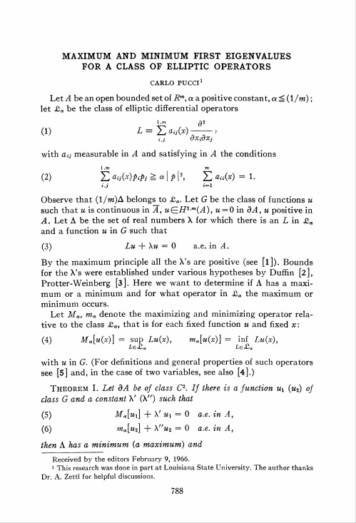
MAXIMUM AND MINIMUM FIRST EIGENVALUES FOR A CLASS OF ELLIPTIC OPERATORSCARLO PUCCI1Let A be an open bounded set of Rm, a a positive constant, a ^ (1/m); let £a be the class of elliptic differential operatorsl,m Q2(1) L—Y1 aii(x)->with an measurable in A and satisfying in A the conditionsl,m m(2) E aij(x)pfpj ^ a | p |2, £ au(x) = 1.i.j i=lObserve that (l/w)A belongs to <£…. L et G be the class of functions u such that u is continuous in A, u^H2-m(A), w = 0 in 3^4, u positive in A. Let A be the set of real numbers X for which there is an L in £a and a function u in G such that(3) Z,« + Xw =0 a.e. in A.By the maximum principle all the X's are positive (see [l]). Bounds for the X's were established under various hypotheses by Duffin [2], Protter-Weinberg [3]. Here we want to determine if A has a maxi-mum or a minimum and for what operator in £… the maximum or minimum occurs.Let Ma, ma denote the maximizing and minimizing operator rela-tive to the class £a, that is for each fixed function u and fixed x: (4) ikf…[tt(x)] = sup Lu(x), ma[u(x)] = inf. Lu(x),with m in G. (For definitions and general properties of such operators see [5] and, in the case of two variables, see also [4].)Theorem I. Let dA be of class C2. If there is a function ui (u2) of class G and a constant X' (X") such that(5) ifa[wi] + X' Mi = 0 a.e. in A,(6) ma[u2] + \"u2 = 0 a.e. in A,then A has a minimum (a maximum) andReceived by the editors February 9, 1966.1 This research was done in part at Louisiana State University. The author thanks Dr. A. Zettl for helpful discussions.788MAXIMUM A ND MINIMUM FIRST EIGENVALUES 789 (7) X' = min A, X" = max A.Theorem II. Let A be the sphere {x: \x\ <1}. Denote with b(c) the first zero of the Bessel function Jp (Jq) where2(m - l)a - 1 1 - 2a(8) P = ~0—^-7T-' q = —tt- ■2 — 2(m — \)a 2aThen(9) min A = [l — (m — l)ct]b2, max A = ac2;the equation for which the minimum occurs isl,*r xx~\ d2U(10) £ '« + (1 - *"*) J1!: -+ [1 - (m - l)a]b2u = 0,ij \_ \ x 12J d XjdXjand a solution of class G is(11) |*|"p/p(&|*|);the equation for which the maximum occurs isl^rl-a ma — 1 XiXj 1d2u(12) Z --S^ +- t^ h-r- + «c*u = 0,ij L« — 1 m — \ \x\lA oxidxjand a solution of class G is(13) | x\-"Jq(c\ x\ ).Observe that for a — \/m there is only the operator (\/m)A in the class £a and by Theorem II it follows that min A = max A = m/b with b the first eigenvalue of -7(m-2) /*Theorem III. Let r\ be the supremum of the radii of the spheres con-tained in A and r2 the infimum of the radii of the spheres containing A. Then for any X in A we have1 — (m — \)a a-b2 < X < — c2,r\ ' ~ r22 1where b, c are defined in Theorem II.First we prove a lemma:Lemma. Let dA be of class C2 and let u in G be a solution of (3) for some L in £a and some real X. Denote by d(x) the distance of x from dA; there are two positive constants kx, k2 such that in A(14) kxd(x) ^ u(x) g k2d(x).790 CARLO P UCCI [August The lemma is substantially known; the proof is based on the stan-dard use of an auxiliary function.By hypothesis there is a constant h such that for any point x" of dA two open spheres Si and S2 of radius h exist such that Si is con-tained in A, S2 has no points in common with A and x° belongs to the closure of both Si and S2. For a fixed x°oi dA let y be the center of S2 and/ h y«(15) g(y) = l- h-r) •\ I x— y I /From (1) it follows thati / h yi". .Lg = Y\Tx~^—\) \x~y\2<16> i^k)hi^m^}and from (2)Lg < — c in A,with c a positive constant depending only on a, h and the diameterof A. Denote by t the maximum of Xw in A; we obtainl(—g — u\ ^ 0 in A, — g — u ^ 0 in dA,and by the maximum principle (see [l])t r / h v/on(17) "s iv - (h^tt) J-For a fixed x in A denote by x° one of the nearest points to x on dA; we have \x — x°\ =d(x), \x — y\ =d(x)+h and by (17) the second inequality of (14) follows for a proper choice of k2.Now let y be the center of the sphere Si relative to a point x" in dA, and letr-(*:y< |*-y| <hj,hs = —- mm m(x);21/a — 1 d(*)&V2it follows that1966] MAXIMUM AND MINIMUM FIRST EIGENVALUES 791u + sg ^ 0 in dTand by (16)L(u + sg) = — Xu+sLg < 0 in T,then again using the maximum principle(18) u(x) ^ si(--r-\ - ll in T.For a fixed x in A, with d(#) <(h/2), denote by x" the nearest point of dA; then |x— y\ =h—d(x) and the first inequality of (14) follows by (18); for x such that d(x) 2? (h/2) it follows by the positivity of u.Proof of Theorem I. Suppose u\ in G is a solution of (5).By a previous result (see [3]) there is an operator L\ in £a such thatMa[«i] = LxUx.Let m be a function of G which is a solution of (3), with L in £a. By the lemmaui(x)inf —-— = t > 0.xeA u(x)We haveX'Xsu — X'tti < 0 in ^4 for s = t — ;Xby (4) we obtainL(su — Ux) ^ Lsu — Ma[ux] = — Xsu + X'«i ^ 0 a.e. in A. Also su — U x =0 in d^l and by the maximum principle su — U x^sO'mA, that isX' 1 ux— g-in A,X t uand X' g=A f ollows by definition of t.A similar proof holds for the maximum of A; in this case we con-siderUi(x)sup->zeA u(x)which is finite by the lemma.Proof of Theorem II. By (8) and (2) it follows that p and q> — 1.792 CARLO PUCCI [August Let r be the distance from the origin and cp(r) the function given by (13). By elementary properties of Bessel functionsx / c \2i+q r2i*(r) = E(-l)*'( — ) -iti \l) UT(i+q+l)and <p i s nonnegative, decreasing and of class C2 in [0,1],(19) 4>'(0) = 0, 0(1) = 0;furthermore <p i s a solution of the equation1 + 2q<t>" +- <t>' + c2<j> = 0,rthat is\-a(20) acj>" -\-4>' + c2a<f> = 0.rWe prove that<t>'(21) <t>"-SO in (0,1].rBy (20)0' 1 <j>'(22) 0"-=-c24>.r a rInequality (21) holds in the limit at r = 0 and, by (22) it holds for r = l. If (21) does not hold1 4>'(23) -c20a rhas a minimum in (0, 1) and its derivative is zero at this point, that is1 <i>" 1 4>'-+ ___ey-o,a r a rland by (20) it follows that at the point of minimum (23) is positive.Let u(x) =<p(r); u belongs to G. Let d[u] be the principal curva-tures of u, i.e. the eigenvalues of the matrix | (d2u)/(dxidxj) \ orderedin the following wayCx[u] ^ C2[u] g • • • S Cm[u].i966] MAXIMUM AND MINIMUM FIRST EIGENVALUES 793By a previous result, see [3],mma[u] = [l — (m — l)a]Ci[«] +a^ d[u].<—1By (21)A'(24) Cm[«] = <b", d[u] = —, i = 1, 2, • • • , m - 1,rthen by (20)ma[u] + c2w = 0 in A.The second equality of (9) follows by Theorem I. Since-= 0" —-—h <b'[-— ),dXidXj r2 \r r3 /(12) follows.The function <p(r) defined by (11) is a solution of(m — l)a r[1 - (m - l)a]<t>" -\-<p' + [1 - (m - l)a]b2<p = 0.rBy the same argument (21) holds and hence also (24) with u(x) =<j>(r). Similarly, usingm—1Ma[u] = [l- (m- l)a]Cm[u] +«S Ct[u],1=1we complete the proof.Proof of Theorem III. Let r be the radius of a sphere S, with A dS. By Theorem II there follows the existence of a function v, vEH2'm(S)r\C°(S), such thatOiC2Mav -\-v = 0, v > 0 in S,r2v = 0 in dS.Letm(x)t = max-«U v(x)where u is a function of class G and a solution of (3) with Z,££a.The nonpositive function m —t v takes its maximum inside A and at that point L(u — tv) gO; but794 CARLO P UCCI [Augustac2 /ac2 \ L(u — tv) ^ —Xu + I-» = X(tv — u) +tv[-X ) in A.r2 \r2 / Henceac2-X < 0.r2Observation I. In Theorem I the hypothesis "Let dA be of class C2" can be replaced by "Let A be star-shaped." The hypothesis of smoothness of the boundary was used only to prove thatUx(x)(25) inf —^- > 0.zeA u(x)Using a dilatation we can replace Ux b y a function v such thatv > 0 in A, Mav 4- Xv = 0 in A,with X a s near as we like to X'. By the argument of the proof of Theo-rem I it follows that X^X and then X^X'.A similar argument holds for the maximum of A.Observation II. In Theorem I the hypothesis "Let dA be of class C2" can be replaced by an hypothesis used by Duffin in a similar problem [2]: "We suppose that a function w of class C2(A) exists such thatw > 1 in A, Maw 4- kw < 0 in dA,where & = sup A."We observe that if (25) holds the proof is the same as before. If (25) does not hold, for e positive and sufficiently smallUx + 6Wutakes its minimum in a point so near to the boundary that there Maw+kw<0. In this point of minimum we must haveUx + ewL-S 0,uand by the hypothesis and some computations it follows that X'^X. The other part of the proof is obtained considering«2u + ew1966] MAXIMUM AND MINIMUM FIRST EIGENVALUES 795 Observation III. Let /3, y denote two nonnegative constants; the previous considerations can be extended to the class £a.a,y of elliptic operators L» dL = Li+ 2^ bi-h c,,=i dXiwith 6,-, c measurable in A and™ 2 2IiG£., Z *.: £(3 , -7 ^ c g 0.1=1The maximizing and minimizing operator related to the class £«,g,y is studied in [5].References1. A. D. Aleksandrov, Certain estimates for the Dirichlet problem, Dokl. Akad. Nauk SSSR 134 (1960), 1001-1004=Soviet Math. Dokl. 1 (1961), 1151-1154.2. R. J. Duffin, Lower bounds for eigenvalues, Phys. Rev. 71 (1947), 827-828.3. M. H. Protter and H. F. Weinberger, On the spectrum of general second order operators, Bull. Amer. Math. Soc. 72 (1966), 251-255.4. C. Pucci, Un problema variazionale per i coefficienti di equazioni differenziali di tipo ellittico, Ann. Scuola Norm. Sup. Pisa 16 (1962), 159-172.5. -, Operatori ellittici estremanti, Ann. Mat. Pura Appl. 72 (1966), 141-170.UniversitA di Genova。

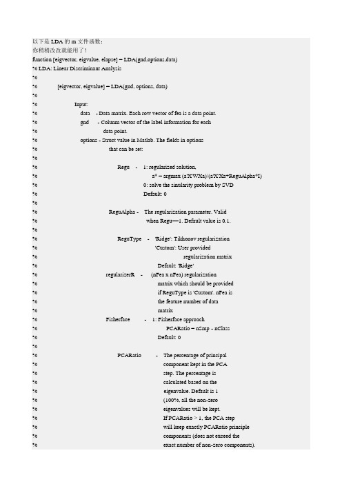
以下是LDA的m文件函数：你稍稍改改就能用了！function [eigvector, eigvalue, elapse] = LDA(gnd,options,data)% LDA: Linear Discriminant Analysis%% [eigvector, eigvalue] = LDA(gnd, options, data)%% Input:% data - Data matrix. Each row vector of fea is a data point.% gnd - Colunm vector of the label information for each% data point.% options - Struct value in Matlab. The fields in options% that can be set:%% Regu - 1: regularized solution,% a* = argmax (a'X'WXa)/(a'X'Xa+ReguAlpha*I) % 0: solve the sinularity problem by SVD% Default: 0%% ReguAlpha - The regularization parameter. Valid% when Regu==1. Default value is 0.1.%% ReguType - 'Ridge': Tikhonov regularization% 'Custom': User provided% regularization matrix% Default: 'Ridge'% regularizerR - (nFea x nFea) regularization% matrix which should be provided% if ReguType is 'Custom'. nFea is% the feature number of data% matrix% Fisherface - 1: Fisherface approach% PCARatio = nSmp - nClass% Default: 0%% PCARatio - The percentage of principal% component kept in the PCA% step. The percentage is% calculated based on the% eigenvalue. Default is 1% (100%, all the non-zero% eigenvalues will be kept.% If PCARatio > 1, the PCA step% will keep exactly PCARatio principle% components (does not exceed the% exact number of non-zero components).%%% Output:% eigvector - Each column is an embedding function, for a new % data point (row vector) x, y = x*eigvector % will be the embedding result of x.% eigvalue - The sorted eigvalue of LDA eigen-problem.% elapse - Time spent on different steps%% Examples:%% fea = rand(50,70);% gnd = [ones(10,1);ones(15,1)*2;ones(10,1)*3;ones(15,1)*4];% options = [];% options.Fisherface = 1;% [eigvector, eigvalue] = LDA(gnd, options, fea);% Y = fea*eigvector;%%% See also LPP, constructW, LGE%%%%Reference:%% P. N. Belhumeur, J. P. Hespanha, and D. J. Kriegman, 揈igenfaces% vs. fisherfaces: recognition using class specific linear% projection,? IEEE Transactions on Pattern Analysis and Machine% Intelligence, vol. 19, no. 7, pp. 711-720, July 1997.%% Deng Cai, Xiaofei He, Yuxiao Hu, Jiawei Han, and Thomas Huang,% "Learning a Spatially Smooth Subspace for Face Recognition", CVPR'2007 %% Deng Cai, Xiaofei He, Jiawei Han, "SRDA: An Efficient Algorithm for% Large Scale Discriminant Analysis", IEEE Transactions on Knowledge and % Data Engineering, 2007.%% version 2.1 --June/2007% version 2.0 --May/2007% version 1.1 --Feb/2006% version 1.0 --April/2004%%if ~exist('data','var')global data;endif (~exist('options','var'))options = [];endif ~isfield(options,'Regu') | ~options.RegubPCA = 1;if ~isfield(options,'PCARatio')options.PCARatio = 1;endelsebPCA = 0;if ~isfield(options,'ReguType')options.ReguType = 'Ridge';endif ~isfield(options,'ReguAlpha')options.ReguAlpha = 0.1;endendtmp_T = cputime;% ====== Initialization[nSmp,nFea] = size(data);if length(gnd) ~= nSmperror('gnd and data mismatch!');endclassLabel = unique(gnd);nClass = length(classLabel);Dim = nClass - 1;if bPCA & isfield(options,'Fisherface') & options.Fisherface options.PCARatio = nSmp - nClass;endif issparse(data)data = full(data);endsampleMean = mean(data,1);data = (data - repmat(sampleMean,nSmp,1));bChol = 0;if bPCA & (nSmp > nFea+1) & (options.PCARatio >= 1) DPrime = data'*data;DPrime = max(DPrime,DPrime');[R,p] = chol(DPrime);if p == 0bPCA = 0;bChol = 1;endend%======================================% SVD%======================================if bPCAif nSmp > nFeaddata = data'*data;ddata = max(ddata,ddata');[eigvector_PCA, eigvalue_PCA] = eig(ddata);eigvalue_PCA = diag(eigvalue_PCA);clear ddata;maxEigValue = max(abs(eigvalue_PCA));eigIdx = find(eigvalue_PCA/maxEigValue < 1e-12);eigvalue_PCA(eigIdx) = [];eigvector_PCA(:,eigIdx) = [];[junk, index] = sort(-eigvalue_PCA);eigvalue_PCA = eigvalue_PCA(index);eigvector_PCA = eigvector_PCA(:, index);%=======================================if options.PCARatio > 1idx = options.PCARatio;if idx < length(eigvalue_PCA)eigvalue_PCA = eigvalue_PCA(1:idx);eigvector_PCA = eigvector_PCA(:,1:idx);endelseif options.PCARatio < 1sumEig = sum(eigvalue_PCA);sumEig = sumEig*options.PCARatio;sumNow = 0;for idx = 1:length(eigvalue_PCA)sumNow = sumNow + eigvalue_PCA(idx);if sumNow >= sumEigbreak;endendeigvalue_PCA = eigvalue_PCA(1:idx);eigvector_PCA = eigvector_PCA(:,1:idx);end%=======================================eigvalue_PCA = eigvalue_PCA.^-.5;data = (data*eigvector_PCA).*repmat(eigvalue_PCA',nSmp,1);elseddata = data*data';ddata = max(ddata,ddata');[eigvector, eigvalue_PCA] = eig(ddata);eigvalue_PCA = diag(eigvalue_PCA);clear ddata;maxEigValue = max(eigvalue_PCA);eigIdx = find(eigvalue_PCA/maxEigValue < 1e-12);eigvalue_PCA(eigIdx) = [];eigvector(:,eigIdx) = [];[junk, index] = sort(-eigvalue_PCA);eigvalue_PCA = eigvalue_PCA(index);eigvector = eigvector(:, index);%=======================================if options.PCARatio > 1idx = options.PCARatio;if idx < length(eigvalue_PCA)eigvalue_PCA = eigvalue_PCA(1:idx);eigvector = eigvector(:,1:idx);endelseif options.PCARatio < 1sumEig = sum(eigvalue_PCA);sumEig = sumEig*options.PCARatio;sumNow = 0;for idx = 1:length(eigvalue_PCA)sumNow = sumNow + eigvalue_PCA(idx);if sumNow >= sumEigbreak;endendeigvalue_PCA = eigvalue_PCA(1:idx);eigvector = eigvector(:,1:idx);end%=======================================eigvalue_PCA = eigvalue_PCA.^-.5;eigvector_PCA = (data'*eigvector).*repmat(eigvalue_PCA',nFea,1);data = eigvector;clear eigvector;endelseif ~bCholDPrime = data'*data;% options.ReguAlpha = nSmp*options.ReguAlpha;switch lower(options.ReguType)case {lower('Ridge')}for i=1:size(DPrime,1)DPrime(i,i) = DPrime(i,i) + options.ReguAlpha;endcase {lower('Tensor')}DPrime = DPrime + options.ReguAlpha*options.regularizerR;case {lower('Custom')}DPrime = DPrime + options.ReguAlpha*options.regularizerR;otherwiseerror('ReguType does not exist!');endDPrime = max(DPrime,DPrime');endend[nSmp,nFea] = size(data);Hb = zeros(nClass,nFea);for i = 1:nClass,index = find(gnd==classLabel(i));classMean = mean(data(index,:),1);Hb (i,:) = sqrt(length(index))*classMean;endelapse.timeW = 0;elapse.timePCA = cputime - tmp_T;tmp_T = cputime;if bPCA[dumpVec,eigvalue,eigvector] = svd(Hb,'econ');eigvalue = diag(eigvalue);eigIdx = find(eigvalue < 1e-3);eigvalue(eigIdx) = [];eigvector(:,eigIdx) = [];eigvalue = eigvalue.^2;eigvector = eigvector_PCA*(repmat(eigvalue_PCA,1,length(eigvalue)).*eigvector);elseWPrime = Hb'*Hb;WPrime = max(WPrime,WPrime');dimMatrix = size(WPrime,2);if Dim > dimMatrixDim = dimMatrix;endif isfield(options,'bEigs')if options.bEigsbEigs = 1;elsebEigs = 0;endelseif (dimMatrix > 1000 & Dim < dimMatrix/10) | (dimMatrix > 500 & Dim < dimMatrix/20) | (dimMatrix > 250 & Dim < dimMatrix/30)bEigs = 1;elsebEigs = 0;endendif bEigs%disp('use eigs to speed up!');option = struct('disp',0);if bCholoption.cholB = 1;[eigvector, eigvalue] = eigs(WPrime,R,Dim,'la',option);else[eigvector, eigvalue] = eigs(WPrime,DPrime,Dim,'la',option);endeigvalue = diag(eigvalue);else[eigvector, eigvalue] = eig(WPrime,DPrime);eigvalue = diag(eigvalue);[junk, index] = sort(-eigvalue);eigvalue = eigvalue(index);eigvector = eigvector(:,index);if Dim < size(eigvector,2)eigvector = eigvector(:, 1:Dim);eigvalue = eigvalue(1:Dim);endendendfor i = 1:size(eigvector,2)eigvector(:,i) = eigvector(:,i)./norm(eigvector(:,i));endelapse.timeMethod = cputime - tmp_T;elapse.timeAll = elapse.timePCA + elapse.timeMethod;。

Ch6. Eigenvalues and Eigenvectors 特徵值與特徵向量(以下所談的所有矩陣均為方陣。

)這個章節主要是在談一個矩陣可否對角化(Diagonalizable)、及如何對角化。

對角化：給定一個矩陣A，如果存在對角矩陣D和可逆矩陣P滿足A=PDP−1，即A跟對角矩陣D相似，則我們說A是可對角化的。

如果一個矩陣A可以對角化，則容易推出AP=PD，考慮AP i(A乘上P的第i行) =PD i=D ii P i(D的第ii元乘上P的第i行)假設P i=v，D ii=μ，可得Av=μv。

注意到這邊的v一定不是0向量(因為P是可逆的)。

由此我們發現，要把矩陣對角化跟找到這樣的μ和v相當有關。

6.1 The Characteristic polynomial 特徵多項式延續剛才的推論，我們可以定義：μ為A的特徵值(Eigenvalue)，v為A對應於μ 的特徵向量(Eigenvector)，兩者會滿足Av=μv。

(注意到μ和v 一定是相對應的。

)將Av=μv移項得(A−μI)v=0，由於v是非零的，可以知道A−μI應該是奇異矩陣(singular)，亦即det(A−μI)=0。

因此我們可以再定義特徵多項式(Characteristic polynomial)：A的特徵多項式為det(A−tI)，通常記做P A(t)或P(t)。

滿足特徵多項式=0 的解即為特徵值。

在找到特徵值μ以後，從式子(A−μI)v=0可以看出v∈N(A−μI)，因此要找到對應的特徵向量的方法，就是去找N(A−μI)的基底(Basis)。

我們又把N(A−μI)記做E A(μ)，稱其為A的μ特徵空間(μ-eigenspace)。

(為什麼可以找基底當特徵向量？因為若v、w皆為對應於μ的特徵向量，則滿足Av=μv、Aw=μw，將兩者相加得A(v+w)=μ(v+w)，表示v+w也是對應於μ的特徵向量。

另外由A(cv)=μ(cv)知v的任何倍數也會是對應於μ的特徵向量。

MATLAB Lecture 4 – Eigenvalues特征值Ref: MATLAB→Mathematics→Matrices and Linear Algebra→Solving Linear Systems of Equationsl Vocabulary:coefficients 系数 characteristic polynomial 特征多项式root 根 characteristic roots 特征根eigenvalues 特征值 eigenvector 特征向量identity matrix 单位阵 decomposition 分解defective matrix 亏损矩阵（即不可对角化矩阵）orthogonal matrix 正交阵 unitary matrix 酉阵nonsymmetric 非对称的 symmetric 对称的roundoff error 舍入误差 diagonalize 对角化conjugate transpose 共轭转置 associate matrix 共轭转置矩阵defective matrix 亏损矩阵（即不可对角化矩阵 not diagonalizable）singular value decomposition 奇异值分解Schur decomposition Schur 分解 similar matrix 相似矩阵geometric multiplicity 几何重数 algebraic multiplicity 代数重数l Some functionseig poly roots schur svdl Eigenvalue & * singular value decomposition² EigenvaluesAn eigenvalue and eigenvector of a square matrix A are a scalar l and a nonzero vector v that satisfy=Av v lEigenvalue DecompositionWith the eigenvalues on the diagonal of a diagonal matrix L and the corresponding eigenvectors forming the columns of a matrix V, we have=LAV VIf V is nonsingular, this becomes the eigenvalue decomposition1=LA V V-A good example is provided by the coefficient matrix of the ordinary differential equation>>A =[ 0 ­6 ­16 2 ­16­5 20 ­10];>> lambda = eig(A) % produces a column vector containing the eigenvalues.lambda =­3.0710­2.4645+17.6008i­2.4645­17.6008i>> [V,D] = eig(A) % computes the eigenvectors and stores the eigenvalues in a …diagonal matrix.V =­0.8326 0.2003­ 0.1394i 0.2003 + 0.1394i­0.3553 ­0.2110­ 0.6447i ­0.2110 + 0.6447i­0.4248 ­0.6930 ­0.6930D =­3.0710 0 00 ­2.4645+17.6008i 00 0 ­2.4645­17.6008iThe first eigenvector is real and the other two vectors are complex conjugates of each other. All three vectors are normalized to have Euclidean length, norm(v,2), equal to one.The matrix V*D*inv(V), which can be written more succinctly as V*D/V, is within roundoff error of A. And, inv(V)*A*V, or V\A*V, is within roundoff error of D.Defective MatricesSome matrices do not have an eigenvector decomposition. These matrices are defective, or not diagonalizable. For example,>>A = [ 6 12 19­9 ­20 ­334 9 15 ];>> [V,D] = eig(A)V =­0.4741 ­0.4082 ­0.40820.8127 0.8165 0.8165­0.3386 ­0.4082 ­0.4082D =­1.0000 0 00 1.0000 00 0 1.0000l = . The second and third columns of V are the same. For There is a double eigenvalue at 1this matrix, a full set of linearly independent eigenvectors does not exist.The optional Symbolic Math Toolbox extends the capabilities of MA TLAB by connecting to Maple, a powerful computer algebra system. One of the functions provided by the toolbox computes the Jordan Canonical Form. This is appropriate for matrices like our example, which is 3­by­3 and has exactly known, integer elements.>> [X,J] = jordan(A)X =­1.7500 1.5000 2.75003.0000 ­3.0000 ­3.0000­1.2500 1.5000 1.2500J =­1 0 00 1 10 0 1The Jordan Canonical Form is an important theoretical concept, but it is not a reliable computational tool for larger matrices, or for matrices whose elements are subject to roundoff errors and other uncertainties.Schur Decomposition in MATLAB Matrix ComputationsThe MATLAB advanced matrix computations do not require eigenvalue decompositions. They are based, instead, on the Schur decomposition'A USU = where U is an orthogonal matrix and S is a block upper triangular matrix with 1­by­1 and 2­by­2 blocks on the diagonal. The eigenvalues are revealed by the diagonal elements and blocks of S, while the columns of U provide a basis with much better numerical properties than a set of eigenvectors . The Schur decomposition of our defective example is>> [U,S] = schur(A)U =­0.4741 0.6648 0.57740.8127 0.0782 0.5774­0.3386 ­0.7430 0.5774S =­1.0000 20.7846 ­44.69480 1.0000 ­0.60960 0 1.0000The double eigenvalue is contained in the lower 2­by­2 block of S.² *Singular Value DecompositionA singular value and corresponding singular vectors of a rectangular matrix A are a scalar s and a pair of vectors u and v that satisfy,' Av u A u vs s == With the singular values on the diagonal of a diagonal matrix S and the corresponding singular vectors forming the columns of two orthogonal matrices U and V , we have,' AV U A U V =S =SSince U and V are orthogonal, this becomes the singular value decomposition'A U V =S The full singular value decomposition of an m ­by­n matrix involves an m ­by­m U , an m ­by­n S , and an n ­by­n V . In other words, U and V are both square and S is the same size as A . If A has many more rows than columns, the resulting U can be quite large, but most of its columns are multiplied by zeros in S . In this situation, the economy sized decomposition saves both time and storage by producing an m ­by­n U , an n ­by­n S and the same V .The eigenvalue decomposition is the appropriate tool for analyzing a matrix when it represents a mapping from a vector space into itself, as it does for an ordinary differential equation. On the other hand, the singular value decomposition is the appropriate tool for analyzing a mapping from one vector space into another vector space, possibly with a different dimension. Most systems of simultaneous linear equations fall into this second category.If A is square, symmetric, and positive definite, then its eigenvalue and singular value decompositions are the same. But, as A departs from symmetry and positive definiteness, the difference between the two decompositions increases. In particular, the singular value decomposition of a real matrix is always real, but the eigenvalue decomposition of a real, nonsymmetric matrix might be complex.>>A =[9 46 82 7];>> [U,S,V] = svd(A) %the full singular value decompositionU =­0.6105 0.7174 0.3355­0.6646 ­0.2336 ­0.7098­0.4308 ­0.6563 0.6194S =14.9359 00 5.18830 0V =­0.6925 0.7214­0.7214 ­0.6925You can verify that U*S*V' is equal to A to within roundoff error.>> [U,S,V] = svd(A,0) %the economy size decomposition is only slightly smaller.U =­0.6105 0.7174­0.6646 ­0.2336­0.4308 ­0.6563S =14.9359 00 5.1883V =­0.6925 0.7214­0.7214 ­0.6925Again, U*S*V' is equal to A to within roundoff error.² MA TLAB>> A = round(10*randn(3))A =­4 3 12­17 ­11 01 12 3>> p_A = poly(A) % computes the coefficients of the characteristic polynomial of A ans =1.0e+003 *0.0010 0.0120 0.0380 2.0310>> r=roots(p_A)r =­16.87812.4391 +10.6951i2.4391­10.6951iWe usually use eig to compute the eigenvalues of a matrix directly.。