matlab实验作业
- 格式:doc
- 大小:820.00 KB
- 文档页数:26
实验1-1 MATLAB 运算基础1. 先求下列表达式的值,然后显示MATLAB 工作空间的使用情况并保存全部变量。
(1) 0122sin851z e =+(2) 221ln(1)2z x x =++,其中2120.455i x +⎡⎤=⎢⎥-⎣⎦(3) 0.30.330.3sin(0.3)ln , 3.0, 2.9,,2.9,3.022a a e e az a a --+=++=--(4) 2242011122123t t z t t t t t ⎧≤<⎪=-≤<⎨⎪-+≤<⎩,其中t =0:0.25:2.5 2. 已知:求下列表达式的值:(1) A+6*B 和A-B+I (其中I 为单位矩阵) (2) A*B 和A.*B (3) A^3和A.^3 (4) A/B 及B\A(5) [A,B]和[A([1,3],:);B^2]3. 设有矩阵A 和B123453166789101769,111213141502341617181920970212223242541311A B ⎡⎤⎡⎤⎢⎥⎢⎥-⎢⎥⎢⎥⎢⎥⎢⎥==-⎢⎥⎢⎥⎢⎥⎢⎥⎢⎥⎢⎥⎣⎦⎣⎦(1) 求它们的乘积C 。
(2) 将矩阵C 的右下角3×2子矩阵赋给D 。
(3) 查看MATLAB 工作空间的使用情况。
1234413134787,2033657327A B --⎡⎤⎡⎤⎢⎥⎢⎥==⎢⎥⎢⎥⎢⎥⎢⎥-⎣⎦⎣⎦4. 完成下列操作:(1) 求[100,999]之间能被21整除的数的个数。
(2) 建立一个字符串向量,删除其中的大写字母。
5. 已知:⎥⎥⎥⎦⎤⎢⎢⎢⎣⎡=987654321a ,分别计算a 的数组平方和矩阵平方,并观察其结果。
6. ⎥⎦⎤⎢⎣⎡-=463521a ,⎥⎦⎤⎢⎣⎡-=263478b ,观察a 与b 之间的六种关系运算的结果。
7. 角度[]604530=x ,求x 的正弦、余弦、正切和余切。

信号与系统MATLAB第一次实验报告一、实验目的1.熟悉MATLAB软件并会简单的使用运算和简单二维图的绘制。
2.学会运用MATLAB表示常用连续时间信号的方法3.观察并熟悉一些信号的波形和特性。
4.学会运用MATLAB进行连续信号时移、反折和尺度变换。
5.学会运用MATLAB进行连续时间微分、积分运算。
6.学会运用MATLAB进行连续信号相加、相乘运算。
7.学会运用MATLAB进行连续信号的奇偶分解。
二、实验任务将实验书中的例题和解析看懂,并在MATLAB软件中练习例题,最终将作业完成。
三、实验内容1.MATLAB软件基本运算入门。
1). MATLAB软件的数值计算:算数运算向量运算:1.向量元素要用”[ ]”括起来,元素之间可用空格、逗号分隔生成行向量,用分号分隔生成列向量。
2.x=x0:step:xn.其中x0位初始值,step表示步长或者增量,xn 为结束值。
矩阵运算:1.矩阵”[ ]”括起来;矩阵每一行的各个元素必须用”,”或者空格分开;矩阵的不同行之间必须用分号”;”或者ENTER分开。
2.矩阵的加法或者减法运算是将矩阵的对应元素分别进行加法或者减法的运算。
3.常用的点运算包括”.*”、”./”、”.\”、”.^”等等。
举例:计算一个函数并绘制出在对应区间上对应的值。
2).MATLAB软件的符号运算:定义符号变量的语句格式为”syms 变量名”2.MATLAB软件简单二维图形绘制1).函数y=f(x)关于变量x的曲线绘制用语:>>plot(x,y)2).输出多个图像表顺序:例如m和n表示在一个窗口中显示m行n列个图像,p表示第p个区域,表达为subplot(mnp)或者subplot(m,n,p)3).表示输出表格横轴纵轴表达范围:axis([xmax,xmin,ymax,ymin])4).标上横轴纵轴的字母:xlabel(‘x’),ylabel(‘y’)5).命名图像就在subplot写在同一行或者在下一个subplot前:title(‘……’)6).输出:grid on举例1:举例2:3.matlab程序流程控制1).for循环:for循环变量=初值:增量:终值循环体End2).while循环结构:while 逻辑表达式循环体End3).If分支:(单分支表达式)if 逻辑表达式程序模块End(多分支结构的语法格式)if 逻辑表达式1程序模块1Else if 逻辑表达式2程序模块2…else 程序模块nEnd4).switch分支结构Switch 表达式Case 常量1程序模块1Case 常量2程序模块2……Otherwise 程序模块nEnd4.典型信号的MATLAB表示1).实指数信号:y=k*exp(a*t)举例:2).正弦信号:y=k*sin(w*t+phi)3).复指数信号:举例:4).抽样信号5).矩形脉冲信号:y=square(t,DUTY) (width默认为1)6).三角波脉冲信号:y=tripuls(t,width,skew)(skew的取值在-1~+1之间,若skew取值为0则对称)周期三角波信号或锯齿波:Y=sawtooth(t,width)5.单位阶跃信号的MATLAB表示6.信号的时移、反折和尺度变换:Xl=fliplr(x)实现信号的反折7.连续时间信号的微分和积分运算1).连续时间信号的微分运算:语句格式:d iff(function,’variable’,n)Function:需要进行求导运算的函数,variable:求导运算的独立变量,n:求导阶数2).连续时间信号的积分运算:语句格式:int(function,’variable’,a,b)Function:被积函数variable:积分变量a:积分下限b:积分上限(a&b默认是不定积分)8.信号的相加与相乘运算9.信号的奇偶分解四、小结这一次实验让我能够教熟悉的使用这个软件,并且能够输入简单的语句并输出相应的结果和波形图,也在一定程度上巩固了c语言的一些语法。

作业一:P55:1.在一个MATLAB命令中,6+7i和6+7*i有何区别?i和I有何区别?解:在MATLAB中6+7i是一个复数常量,6+7*i则是一个表达式。
i是虚数单位,而I是单位向量。
4.要产生均值为3,方差为1的500个正态分布的随机序列,写出相应的表达式。
解:y=3+sqrt(1)*randn(500)5.求下列矩阵的对角线元素、上三角矩阵、逆矩阵、行列式的值、秩、迹。
(1) A =1 -12 35 1 -4 23 0 5 211 15 0 9(2) B =0.43 43 2-8.9 4 21解:(1)A=[1,-1,2,3;5,1,-4,2;3,0,5,2;11,15,0,9]主对角元素:D=diag(A)上三角矩阵:B=triu(A)下三角矩阵:C=tril(A)逆矩阵:X=inv(A)行列式的值:E=det(A)秩:F=rank(A)逆:G=trace(A)运行结果:A =1 -12 35 1 -4 23 0 5 211 15 0 9主对角元素:D =1159上三角矩阵:B =1 -12 30 1 -4 20 0 5 20 0 0 9下三角矩阵:C =1 0 0 05 1 0 03 0 5 011 15 0 9逆矩阵:X =-0.1758 0.1641 0.2016 -0.0227 -0.1055 -0.1016 -0.0391 0.0664 -0.0508 -0.0859 0.1516 0.0023 0.3906 -0.0313 -0.1813 0.0281 行列式的值:E =1280秩:F =4逆:G =16(2)B = [0.43,43,2;-8.9,4,21]主对角元素:D=diag(B)上三角矩阵:Y=triu(B)下三角矩阵:C=tril(B)逆矩阵:X=pinv(B)行列式的值:E=det(B)秩:F=rank(B)迹:G= trace(B)运行结果:B =0.4300 43.0000 2.0000-8.9000 4.0000 21.0000主对角元素:D =0.43004.0000上三角矩阵:Y =0.4300 43.0000 2.00000 4.0000 21.0000下三角矩阵:C =0.4300 0 0-8.9000 4.0000 0逆矩阵:X =0.0022 -0.01750.0234 -0.0017-0.0035 0.0405行列式的值:E = 1.2526e+003秩:F=3迹:G =5.43006. 当A=[34,NaN,Inf,-Inf,-pi,eps,0]时,求函数all(A)、any(A)、isnan(A)、isinf(A)、isfinite(A)的值。

基于MATLAB 模拟演示衍射实验阚亮亮 李宗景 吴小龙 尹岩 将matlab 应用与以前学习过的课程是学习该课程的最重要的意义,通过matlab 演示衍射实验效果好,简洁,直观。
下图是单缝衍射是matlab 所得到的图像-0.025-0.02-0.015-0.01-0.0050.0050.010.0150.020.025附上MATLAB 程序:lamda=500e-9; %波长N=1; %缝数 ,可以随意更改变换a=2e-4;D=5;d=5*a;ym=2*lamda*D/a;xs=ym;%屏幕上y 的范围n=1001;%屏幕上的点数ys=linspace(-ym,ym,n);%定义区域for i=1:nsinphi=ys(i)/D;alpha=pi*a*sinphi/lamda;beta=pi*d*sinphi/lamda;B(i,:)=(sin(alpha)./alpha).^2.*(sin(N*beta)./sin(beta)).^2;B1=B/max(B);endNC=256; %确定灰度的等级Br=(B/max(B))*NC;subplot(1,2,1)image(xs,ys,Br);colormap(hot(NC)); %色调处理subplot(1,2,2)plot(B1,ys,'k');衍射现象的模拟结果与讨论在实验时改变N的值可以得到单缝以及多缝衍射的输出结果,并可以得到这样的结论:(1)当入射光波长一定时,单缝宽度a越小,衍射条纹越宽,衍射现象越显著;(2)单缝越宽,衍射越不明显,单缝宽度逐渐增大,衍射条纹越来越窄;(3)当缝宽a>>λ时,各级衍射条纹向中央明纹靠拢,而无法分辨,这时衍射现象消失。
结束语利用MATLAB对抽象物理现象进行计算机仿真时,首先必须对物理过程进行数学抽象,建立适合程序实现的数学模型,其次利用MATLAB软件包中的有关工具编制m文件,最后对物理过程和物理现象进行模拟,从而可以把抽象的物理问题进行简明、直观的动态展现。
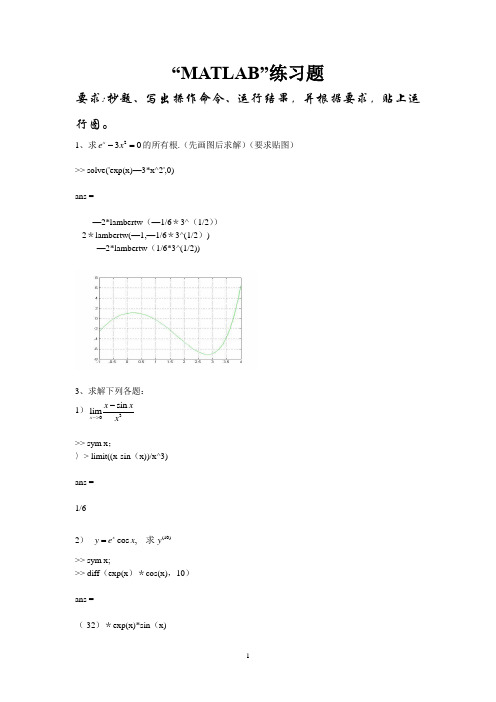
“MATLAB”练习题要求:抄题、写出操作命令、运行结果,并根据要求,贴上运行图。
1、求230x e x -=的所有根.(先画图后求解)(要求贴图)>> solve('exp(x)—3*x^2',0)ans =—2*lambertw (—1/6*3^(1/2))-2*lambertw(—1,—1/6*3^(1/2))—2*lambertw (1/6*3^(1/2))3、求解下列各题:1)30sin lim x x x x ->->> sym x ;〉> limit((x-sin (x))/x^3)ans =1/62) (10)cos ,x y e x y =求>> sym x;>> diff (exp(x )*cos(x),10)ans =(-32)*exp(x)*sin (x)3)21/20(17x e dx ⎰精确到位有效数字)〉〉 sym x;〉〉 vpa((int(exp(x^2),x,0,1/2)),17)ans =0.544987104183622224)42254x dx x+⎰〉> sym x ;>〉 int (x^4/(25+x^2),x)ans =125*atan (x/5) - 25*x + x^3/35)求由参数方程arctan x y t⎧⎪=⎨=⎪⎩dy dx 与二阶导数22d y dx 。
〉> sym t;>> x=log(sqrt (1+t^2));y=atan(t);〉> diff (y ,t )/diff (x ,t)ans =1/t6)设函数y =f (x )由方程xy +e y = e 所确定,求y ′(x ).>> syms x y ;f=x *y+exp(y )—exp (1);〉> -diff(f,x )/diff (f,y)ans =-y/(x + exp (y))7)0sin 2x e xdx +∞-⎰>〉 syms x ;>〉 y=exp(-x)*sin(2*x );〉> int(y ,0,inf )ans =2/58) 08x =展开(最高次幂为)〉> syms xf=sqrt(1+x);taylor(f,0,9)ans =— (429*x^8)/32768 + (33*x^7)/2048 — (21*x^6)/1024 +(7*x^5)/256 - (5*x^4)/128 + x^3/16 - x^2/8 + x/2 + 19) 1sin (3)(2)x y e y =求〉> syms x y ;>〉 y=exp(sin (1/x));>〉 dy=subs (diff(y,3),x ,2)dy =—0.582610)求变上限函数2x x ⎰对变量x 的导数.>> syms a t ;>〉 diff (int(sqrt(a+t),t,x ,x^2))Warning: Explicit integral could not be found 。

实验一MATLAB运算基础1、用逻辑表达式求下列分段函数的值。
t=0:0.5:2.5y=t.^2.*((t>=0)&(t<1))+(t.^2-1).*(( t>=1)&(t<2))+(t.^2-2*t+1).*((t>=2 )&(t<3))2、求[100,999]之间能被21整除的数的个数。
p=rem([100:999],21)==0;sum(p)3、建立一个字符串向量,删除其中的大写字母。
ch='KdDdfKaWdsfCI',k=find(ch>=' A'&ch<='Z'),ch(k)=[]4、输入矩阵,并找出A中大于或等于5的元素。
A=[1 2 3;4 5 6;7 8 9],[m,n]=find(A>=5),for j=1:length(m)x(j)=A(m(j),n(j))xend5、求矩阵的行列式值、逆和特征根。
a11=input('a11='),a12=input('a12 ='),a21=input('a21='),a22=input('a22 ='),A=[a11,a12;a21,a22],DA=det(A),IA=inv(A),EA=eig(A) 6、不采用循环的形式求出和式的数值解。
sum(2.^[0:63])实验二1、1行100列的Fibonacc数组a,a(1)=a(2)=1,a(i)=a(i-1)+a(i-2),用for循环指令来寻求该数组中第一个大于10000的元素,并指出其位置i。
n=100;a=ones(1,n);for i=3:na(i)=a(i-1)+a(i-2);if a(i)>10000a(i),break;end;end,i2、编写M脚本文件,定义下列分段函数,并分别求出当()、()和()时的函数值。
MATLAB实验大作业学院:数理与信息工程学院专业:电子与信息工程班级:学号:姓名:联系方式:指导老师:许秀玲成绩:仿真模块设计汽车沿直线山坡向上行驶,要求设计一个简单的比例放大器,使汽车能以指定的速度运动。
其中牵引力Fe最大为1000,最大制动力为2000,即-2000<Fe<1000。
空气阻力为Fw=0.001(v+20sin(0.001t))2,v为速度,重力分量为Fh=30sin(0.0001x),x为位移。
汽车质量m为100个单位。
分析:汽车的运动方程:x’’=(Fe-Fw-Fh)/m式(1)要达到使汽车以指定的速度行驶,可以采用PID控制,即将期望速度与实际速度相比较,以它们的差的某一倍数为牵引力驱动汽车。
即Fe=Kp(v*-v)式(2)又Fw=0.001(v+20sin(0.001t))2式(3)Fh=30sin(0.0001x)式(4)将式(2)、(3)、(4)代入方程(1)可建立运动方程,设期望速度v*为70。
根据运动方程即可建立仿真模型,如下图1.1所示:图1.1 仿真模型图建立仿真模型后,其中Fcn为空气阻力分量Fw,参数设置如图1.2所示:图1.2 Fcn参数设置Fcn1为空气阻力分量Fh,参数设置如图1.3所示:图1.3Fcn1参数设置各个模块作用分析:Add模块:该模块的作用是得到期望速度与实际速度的差,再乘以后面Gain 模块的50,即得到牵引力Fe。
MinMax模块:该模块的作用是比较Fe与最大牵引力1000的大小。
如果Fe 小于1000则输出,大于1000则不输出。
MinMax1模块:该模块的作用是比较输出的Fe与最大制动力2000的大小。
如果Fe大于2000则输出,小于2000则不输出。
MinMax模块和MinMax1模块共同作用,筛选符合题目要求的Fe。
Add1模块:Add1模块的输入分别为Fe、Fh、Fw,输出为汽车所受的合外力为:F=Fe-Fw-Fh再经过后面的Gain1模块乘以0.01,即根据合外力公式:F=ma得,加速度等于合外力除以质量m=100,即得到x’’。
实验一 典型连续时间信号和离散时间信号一、实验目的掌握利用Matlab 画图函数和符号函数显示典型连续时间信号波形、典型时间离散信号、连续时间信号在时域中的自变量变换。
二、实验内容1、典型连续信号的波形表示(单边指数信号、复指数信号、抽样信号、单位阶跃信号、单位冲击信号)1)画出教材P28习题1-1(3) ()[(63)(63)]t f t e u t u t =----的波形图。
function y=u(t) y=t>=0;t=-3:0.01:3;f='exp(t)*(u(6-3*t)-u(-6-3*t))';ezplot(f,t);grid on;2)画出复指数信号()()j t f t e σω+=当0.4, 8σω==(0<t<10)时的实部和虚部的波形图。
t=0:0.01:10;f1='exp(0.4*t)*cos(8*t)';f2='exp(0.4*t)*sin(8*t)';figure(1)ezplot(f1,t);grid on;figure(2)ezplot(f2,t);grid on;t=-10:0.01:10; f='sin(t)/t'; ezplot(f,t); grid on;t=0:0.01:10;f='(sign(t-3)+1)/2'; ezplot(f,t);grid on;5)单位冲击信号可看作是宽度为∆,幅度为1/∆的矩形脉冲,即t=t 1处的冲击信号为11111 ()()0 t t t x t t t otherδ∆⎧<<+∆⎪=-=∆⎨⎪⎩画出0.2∆=, t 1=1的单位冲击信号。
t=0:0.01:2;f='5*(u(t-1)-u(t-1.2))';ezplot(f,t);grid on;axis([0 2 -1 6]);2、典型离散信号的表示(单位样值序列、单位阶跃序列、实指数序列、正弦序列、复指数序列)编写函数产生下列序列:1)单位脉冲序列,起点n0,终点n f,在n s处有一单位脉冲。
MATLAB绘图作业作业内容:1、请用三种不同的方法将三条曲线同时绘制在一个figure窗口(提示:其中有一种是用subplot),并在每一条曲线的旁边加上曲线的公式,这三条曲线的公式、颜色和线形均由你们定,但是,横轴,也就是x轴都是[-10,10],间隔为0.5。
法一:x=-10:0.5:10;y=sin(x);z=cos(x);w=tan(x);subplot(1,3,[1,2,3]);plot(x,y,'r-',x,z,'b--',x,w,'g+')gtext('sin(x)');gtext('cos(x)');gtext('tan(x)');法二:x=-10:0.5:10;y=sin(x);z=cos(x);w=tan(x);plot(x,y,'r-');hold on;plot(x,z,'b--');hold on;plot(x,w,'k+');gtext('sin(x)');gtext('cos(x)');gtext('tan(x)');法三:x=-10:0.5:10;y=sin(x);z=cos(x);w=tan(x);plot(x,y,'r-',x,z,'b--',x,w,'c+');gtext('sin(x)');gtext('cos(x)');gtext('tan(x)');2、还是这道题,不使用subplot方法将三条曲线绘制在同一个figure窗口中,然后为它们增加标注、标题、横坐标、纵坐标的名称(随便你们想),再加上网格。
x=-10:0.5:10;y=sin(x);z=cos(x);w=tan(x);plot(x,y,'r-',x,z,'b--',x,w,'c+');title('图形');xlabel('横坐标');ylabel('纵坐标');grid on;legend('正弦','余弦','正切','location','northeastoutside');gtext('sin(x)');gtext('cos(x)');gtext('tan(x)');3、x=[-20, 20], 间隔1,函数y=2x2-3x+10,请用fplot函数来绘制该曲线,函数名由你来定。
MATLAB实验报告第一部分第二题、A=[1 2 3 4;4 3 2 1;2 3 4 1;3 2 4 1]A =1 2 3 44 3 2 12 3 4 13 24 1>> A(5,6)=5A =1 2 3 4 0 04 3 2 1 0 02 3 4 1 0 03 24 1 0 00 0 0 0 0 5B=[1+4j 2+3j 3+2j 4+1j;4+1j 3+2j 2+3j 1+4j;2+3j 3+2j 4+1j 1+4j;3+2j 2+3j 4+1j 1+4j]B =1.0000 + 4.0000i2.0000 +3.0000i 3.0000 + 2.0000i4.0000 + 1.0000i4.0000 + 1.0000i 3.0000 + 2.0000i 2.0000 + 3.0000i 1.0000 + 4.0000i2.0000 +3.0000i 3.0000 + 2.0000i4.0000 + 1.0000i 1.0000 + 4.0000i3.0000 + 2.0000i 2.0000 + 3.0000i4.0000 + 1.0000i 1.0000 + 4.0000i >>第三题、>> A=magic(8)A =64 2 3 61 60 6 7 579 55 54 12 13 51 50 1617 47 46 20 21 43 42 2440 26 27 37 36 30 31 3332 34 35 29 28 38 39 2541 23 22 44 45 19 18 4849 15 14 52 53 11 10 568 58 59 5 4 62 63 1>> B=A(2:2:end,:)B =9 55 54 12 13 51 50 1640 26 27 37 36 30 31 3341 23 22 44 45 19 18 488 58 59 5 4 62 63 1第四题、s=0;n=0;while(n<=63),s=s+2^n;n=n+1;end,ss =1.8447e+019或者s=0;for i=1:63,s=s+2^i;end,ss =1.8447e+19或者sum(sym(2.^[1:63]))ans =18446744073709551614第五题、>> t=[-1:0.01:1];>> y=sin(1./t);>> plot(t,y)调整步距后:t=[-1:0.03:-0.25,-0.248:0.001:0.248,0.25:0.03:1]; >> y=sin(1./t);>>plot(t,y)t=[-pi:0.01:pi];y=sin(tan(t))-tan(sin(t));plot(t,y)调整步距后:>>t=[-pi:0.05:-1.8,-1.799:0.001:-1.2,-1.2:0.05:1.2,1.201:0.001:1.8,1.81:0.05:pi]; y=sin(tan(t))-tan(sin(t));plot(t,y)第六题、[x,y]=meshgrid(-2:0.1:2);z=1./(sqrt((1-x).^2+y.^2))+1./(sqrt((1+x).^2+y.^2));surf(x,y,z),shading flatWarning: Divide by zero.Warning: Divide by zero.xx=[-2:.1:-1.2,-1.1:0.02:-0.9,-0.8:0.1:0.8,0.9:0.02:1.1,1.2:0.1:2];yy=[-1:0.1:-0.2,-0.1:0.02:0.1,0.2:.1:1];[x,y]=meshgrid(xx,yy);z=1./(sqrt((1-x).^2+y.^2))+1./(sqrt((1+x).^2+y.^2));surf(x,y,z),shading flat;zlim([0,15])xx=[-2:.1:-1.2,-1.1:0.02:-0.9,-0.8:0.1:0.8,0.9:0.02:1.1,1.2:0.1:2];yy=[-1:0.1:-0.2,-0.1:0.02:0.1,0.2:.1:1];[x,y]=meshgrid(xx,yy);z=1./(sqrt((1-x).^2+y.^2))+1./(sqrt((1+x).^2+y.^2));surf(x,y,z),shading flat;zlim([0,15])xx=[-2:0.1:-1.2,-1.1:0.02:-0.9,-0.8:0.1:0.8,0.9:0.02:1.1,1.2:0.1:2];yy=[-1:0.1:-0.2,-0.1:0.02:0.1,0.2:0.1:1];[x,y]=meshgrid(xx,yy);z=1./(sqrt((1-x).^2+y.^2))+1./(sqrt((1+x).^2+y.^2));subplot(224),surf(x,y,z)subplot(221),surf(x,y,z),view(0,90)%俯视图subplot(222),surf(x,y,z),view(90,0)%侧视图subplot(223),surf(x,y,z),view(0,0) %正视图>>第七题(1)syms x;>> f=(3.^x+9.^x).^(1/x);>> L1=limit(f,x,inf)L1 =9(2)syms x y;f=(x.*y)./(sqrt(x.*y+1)-1);L1=limit(limit(f,x,0),y,0)L1 =2(3)syms x y;f=(1-cos(x.^2+y.^2))./(x.^2+y.^2*exp(x.^2+y.^2));L1=limit(limit(f,x,0),y,0) L1 =第八题>> syms t;x=log(cos(t));y=cos(t)-t*sin(t);>> diff(y,t)/diff(x,t)ans =-(-2*sin(t)-t*cos(t))/sin(t)*cos(t)>> f=diff(y,t,2)/diff(x,t,2);subs(f,t,sym(pi)/3)ans =3/8-1/24*pi*3^(1/2)第九题>> syms x y t>> f=int(exp(-t^2),t,0,x*y);>> x/y*diff(f,x,2)-2*diff(diff(f,x),y)+diff(f,y,2)ans =2*x^2*y^2*exp(-x^2*y^2)-2*exp(-x^2*y^2)-2*x^3*y*exp(-x^2*y^2)第十题(1)>> syms k n; limit(symsum(1/((2*k)^2-1),k,1,n),n,inf)ans =1/2(2)>> syms k n;>> limit(n*symsum(1/(n^2+k*pi),k,1,n),n,inf)ans =1第十一题>> syms a t;x=a*(cos(t)+t*sin(t));y=a*(sin(t)-t*cos(t)); >> f=x^2+y^2;I=int(f*sqrt(diff(x,t)^2+diff(y,t)^2),t,0,2*pi)I =2*a^2*pi^2*(a^2)^(1/2)+4*a^2*pi^4*(a^2)^(1/2)>> syms x y a b c t;x=c*cos(t)/a;y=c*sin(t)/b;>> P=y*x^3+exp(y);Q=x*y^3+x*exp(y)-2*y;>> ds=[diff(x,t);diff(y,t)];I=int([P Q]*ds,t,0,pi)I =-2/15*c*(-2*c^4+15*b^4)/b^4/a第十二题编写一个vander()函数如下:function A=vander(v)n=length(v);v=v(:);A=sym(ones(n));for j=n-1:-1:1,A(:,j)=v.*A(:,j+1);end>> syms a b c d e;A=vander([a b c d e])A =[ a^4, a^3, a^2, a, 1][ b^4, b^3, b^2, b, 1][ c^4, c^3, c^2, c, 1][ d^4, d^3, d^2, d, 1][ e^4, e^3, e^2, e, 1]>> det(A),simple(ans)ans =(c-d)*(b-d)*(b-c)*(a-d)*(a-c)*(a-b)*(-d+e)*(e-c)*(e-b)*(e-a)第十三题>> A=[-2,0.5,-0.5,0.5;0,-1.5,0.5,-0.5;2,0.5,-4.5,0.5;2,1,-2,-2];[V J]=jordan(sym(A)) V =[ 0, 1/2, 1/2, -1/4][ 0, 0, 1/2, 1][ 1/4, 1/2, 1/2, -1/4][ 1/4, 1/2, 1, -1/4]J =[ -4, 0, 0, 0][ 0, -2, 1, 0][ 0, 0, -2, 1][ 0, 0, 0, -2]第十四题A=[3,-6,-4,0,5;1,4,2,-2,4;-6,3,-6,7,3;-13,10,0,-11,0;0,4,0,3,4];B=[3,-2,1;-2,-9,2;-2,-1,9];C=-[-2,1,-1;4,1,2;5,-6,1;6,-4,-4;-6,6,-3];X=lyap(A,B,C)X =4.0569 14.5128 -1.5653-0.0356 -25.0743 2.7408-9.4886 -25.9323 4.4177-2.6969 -21.6450 2.8851-7.7229 -31.9100 3.7634>> norm(A*X+X*B+C)ans =3.9251e-13X=lyap(sym(A),B,C)X =[ -434641749950/107136516451, -4664546747350/321409549353, 503105815912/321409549353][ 3809507498/107136516451, 8059112319373/321409549353, -880921527508/321409549353][ 1016580400173/107136516451, 8334897743767/321409549353, -1419901706449/321409549353][ 288938859984/107136516451, 6956912657222/321409549353, -927293592476/321409549353][ 827401644798/107136516451, 10256166034813/321409549353, -1209595497577/321409549353]>> A*X+X*B+Cans =[ 0, 0, 0][ 0, 0, 0][ 0, 0, 0][ 0, 0, 0][ 0, 0, 0]>>第十五题(1)>> syms t;A=[-4.5,0,0.5,-1.5;-0.5,-4,0.5,-0.5;1.5,1,-2.5,1.5;0,-1,-1,-3];B=simple(expm(A*t))B =[ (exp(-5*t)*(exp(2*t) - t*exp(2*t) + t^2*exp(2*t) + 1))/2, (exp(-5*t)*(2*t*exp(2*t) - exp(2*t) + 1))/2, (t*exp(-3*t)*(t + 1))/2, -(exp(-5*t)*(exp(2*t) + t*exp(2*t) - t^2*exp(2*t) - 1))/2][ (exp(-5*t)*(t*exp(2*t) - exp(2*t) + 1))/2, (exp(-5*t)*(exp(2*t) + 1))/2, (t*exp(-3*t))/2,(exp(-5*t)*(t*exp(2*t) - exp(2*t) + 1))/2][ (exp(-5*t)*(exp(2*t) + t*exp(2*t) - 1))/2, (exp(-5*t)*(exp(2*t) - 1))/2, (exp(-3*t)*(t + 2))/2, (exp(-5*t)*(exp(2*t) + t*exp(2*t) - 1))/2][ -(t^2*exp(-3*t))/2, -t*exp(-3*t), -(t*exp(-3*t)*(t + 2))/2, -(exp(-3*t)*(t^2 - 2))/2](2)>> syms t;A=[-4.5,0,0.5,-1.5;-0.5,-4,0.5,-0.5;1.5,1,-2.5,1.5;0,-1,-1,-3];j=sym(sqrt(-1));Y=simple((expm(A*j*t)-expm(-A*j*t))/(2*j))Y =[ (t^2*sin(3*t))/2 - sin(5*t)/2 - (t*cos(3*t))/2 - sin(3*t)/2, sin(3*t)/2 - sin(5*t)/2 + t*cos(3*t), (t*cos(3*t))/2 + (t^2*sin(3*t))/2, sin(3*t)/2 - sin(5*t)/2 - (t*cos(3*t))/2 + (t^2*sin(3*t))/2][ sin(3*t)/2 - sin(5*t)/2 + (t*cos(3*t))/2, -4*sin(t)*(2*sin(t)^4 - 3*sin(t)^2 + 1), (t*cos(3*t))/2, sin(3*t)/2 - sin(5*t)/2 + (t*cos(3*t))/2][ sin(5*t)/2 - sin(3*t)/2 + (t*cos(3*t))/2, sin(t) + 8*sin(t)^3*(sin(t)^2 - 1), (t*cos(3*t))/2 - sin(3*t), sin(5*t)/2 - sin(3*t)/2 + (t*cos(3*t))/2][ -(t^2*sin(3*t))/2, -t*cos(3*t), - t*cos(3*t) - (t^2*sin(3*t))/2, -(sin(3*t)*(t^2 + 2))/2](3)>> syms t;A=[-4.5,0,0.5,-1.5;-0.5,-4,0.5,-0.5;1.5,1,-2.5,1.5;0,-1,-1,-3];B=simple(expm(A*t));j=sym(sqrt(-1));Y=(expm(A*A*j*t*B)-expm(-A*A*j*t*B))/(2*j);X=simple(B*Y)X =[ (exp(-5*t)*sin(25*t*exp(-5*t)))/2 + exp(-9*t)*sin(9*t*exp(-3*t))*(t^4*((81*i)/4) + t^3*(-27*i) + t^2*(9*i))*2*i - exp(-3*t)*sin(9*t*exp(-3*t))*(t^2*(i/4) + t*(-i/4) + i/4)*2*i + 2*exp(-6*t)*cos(9*t*exp(-3*t))*((27*t^3)/4 - (33*t^2)/4 + 2*t), (exp(-5*t)*sin(25*t*exp(-5*t)))/2 - exp(-3*t)*sin(9*t*exp(-3*t))*((t*i)/2 - i/4)*2*i - 2*exp(-6*t)*cos(9*t*exp(-3*t))*(3*t - (9*t^2)/2), 54*t^3*exp(-9*t)*sin(9*t*exp(-3*t)) - 18*t^2*exp(-9*t)*sin(9*t*exp(-3*t)) - (81*t^4*exp(-9*t)*sin(9*t*exp(-3*t)))/2 - (t*exp(-3*t)*sin(9*t*exp(-3*t))*(t*i + i)*i)/2 -(t*exp(-6*t)*cos(9*t*exp(-3*t))*(- 27*t^2 + 15*t + 4))/2, (exp(-5*t)*sin(25*t*exp(-5*t)))/2 + exp(-9*t)*sin(9*t*exp(-3*t))*(t^4*((81*i)/4) + t^3*(-27*i) + t^2*(9*i))*2*i + exp(-3*t)*sin(9*t*exp(-3*t))*((t*i)/4 - (t^2*i)/4 + i/4)*2*i + 2*exp(-6*t)*cos(9*t*exp(-3*t))*((27*t^3)/4 - (33*t^2)/4 + 2*t)][(exp(-5*t)*sin(25*t*exp(-5*t)))/2 - exp(-3*t)*sin(9*t*exp(-3*t))*((t*i)/4 - i/4)*2*i - 2*exp(-6*t)*cos(9*t*exp(-3*t))*((3*t)/2 - (9*t^2)/4),(exp(-3*t)*sin(9*t*exp(-3*t)))/2 + (exp(-5*t)*sin(25*t*exp(-5*t)))/2, (t*exp(-6*t)*(exp(3*t)*sin(9*t*exp(-3*t)) - 6*cos(9*t*exp(-3*t)) + 9*t*cos(9*t*exp(-3*t))))/2, (exp(-5*t)*sin(25*t*exp(-5*t)))/2 - exp(-3*t)*sin(9*t*exp(-3*t))*((t*i)/4 - i/4)*2*i - 2*exp(-6*t)*cos(9*t*exp(-3*t))*((3*t)/2 - (9*t^2)/4)][- (exp(-5*t)*sin(25*t*exp(-5*t)))/2 - exp(-3*t)*sin(9*t*exp(-3*t))*((t*i)/4 + i/4)*2*i - 2*exp(-6*t)*cos(9*t*exp(-3*t))*((3*t)/2 - (9*t^2)/4),(exp(-3*t)*sin(9*t*exp(-3*t)))/2 - (exp(-5*t)*sin(25*t*exp(-5*t)))/2, (9*t^2*exp(-6*t)*cos(9*t*exp(-3*t)))/2 - 3*t*exp(-6*t)*cos(9*t*exp(-3*t)) - exp(-3*t)*sin(9*t*exp(-3*t))*((t*i)/4 + i/2)*2*i, - (exp(-5*t)*sin(25*t*exp(-5*t)))/2 - exp(-3*t)*sin(9*t*exp(-3*t))*((t*i)/4 + i/4)*2*i - 2*exp(-6*t)*cos(9*t*exp(-3*t))*((3*t)/2 - (9*t^2)/4)][ 18*t^2*exp(-9*t)*sin(9*t*exp(-3*t)) - (t^2*exp(-3*t)*sin(9*t*exp(-3*t)))/2 - 54*t^3*exp(-9*t)*sin(9*t*exp(-3*t)) + (81*t^4*exp(-9*t)*sin(9*t*exp(-3*t)))/2 - (t*exp(-6*t)*cos(9*t*exp(-3*t))*(27*t^2 - 24*t + 2))/2, -t*exp(-6*t)*(exp(3*t)*sin(9*t*exp(-3*t)) - 6*cos(9*t*exp(-3*t)) + 9*t*cos(9*t*exp(-3*t))), 18*t^2*exp(-9*t)*sin(9*t*exp(-3*t)) - 54*t^3*exp(-9*t)*sin(9*t*exp(-3*t)) + (81*t^4*exp(-9*t)*sin(9*t*exp(-3*t)))/2 + (t*exp(-3*t)*sin(9*t*exp(-3*t))*(t*i + 2*i)*i)/2 + (t*exp(-6*t)*cos(9*t*exp(-3*t))*(- 27*t^2 + 6*t + 10))/2, 18*t^2*exp(-9*t)*sin(9*t*exp(-3*t)) + exp(-3*t)*sin(9*t*exp(-3*t))*(t^2*(i/4) - i/2)*2*i - 2*exp(-6*t)*cos(9*t*exp(-3*t))*((27*t^3)/4 - 6*t^2 + t/2) - 54*t^3*exp(-9*t)*sin(9*t*exp(-3*t)) + (81*t^4*exp(-9*t)*sin(9*t*exp(-3*t)))/2]第二部分第一题>> syms a t;f=sin(a*t)/t;laplace(f)ans =atan(a/s)>> syms t a;f=t^5*sin(a*t);laplace(f)ans =120/(s^2+a^2)^3*sin(6*atan(a/s))>> syms t a;f=t^8*cos(a*t);laplace(f)ans =40320/(s^2+a^2)^(9/2)*cos(9*atan(a/s))第二题>> syms s a b;F=1/(sqrt(s^2)*(s^2-a^2)*(s+b));ilaplace(F)ans =-1/2/(a-b)/a^2*exp(-a*t)+1/b/(a^2-b^2)*exp(-b*t)+1/2/(a+b)/a^2*exp(a*t)-1/a^2/b >> syms s a b;F=sqrt(s-a)-sqrt(s-b);ilaplace(F)ans =1/2/t/(t*pi)^(1/2)*(exp(b*t)-exp(a*t))>> syms a b s;F=log((s-a)/(s-b));ilaplace(F)ans =(exp(b*t)-exp(a*t))/t第三题(1)>> syms x;f=x^2*(3*sym(pi)-2*abs(x));F=fourier(f)F =-6*(4+pi^2*dirac(2,w)*w^4)/w^4>> ifourier(F)ans =x^2*(-4*x*heaviside(x)+3*pi+2*x)(2)>> syms t;f=t^2*(t-2*sym(pi))^2;F=fourier(f)F =2*pi*(dirac(4,w)+4*i*pi*dirac(3,w)-4*pi^2*dirac(2,w)) >> ifourier(F)ans =x^2*(-2*pi+x)^2第四题(1)>> syms k a T;f=cos(k*a*T);F=ztrans(f)F =(z-cos(a*T))*z/(z^2-2*z*cos(a*T)+1)>> f1=iztrans(F)f1 =cos(a*T*n)(2)>> sym k T a;f=(k*T)^2*exp(-a*k*T);F=ztrans(f) F =T^2*z*exp(-a*T)*(z+exp(-a*T))/(z-exp(-a*T))^3>> f1=iztrans(F)f1 =T^2*(1/exp(a*T))^n*n^2(3)>> syms a k T;f=(a*k*T-1+exp(-a*k*T))/a;F=ztrans(f) F =1/a*(a*T*z/(z-1)^2-z/(z-1)+z/exp(-a*T)/(z/exp(-a*T)-1)) >> iztrans(F)ans =((1/exp(a*T))^n+a*T*n-1)/a第五题(1)>> syms x;x1=solve('exp(-(x+1)^2+pi/2)*sin(5*x+2)')x1 =-2/5>> subs('exp(-(x+1)^2+pi/2)*sin(5*x+2)',x,x1)ans =>> f=inline('exp(-(x+1).^2+pi/2).*sin(5*x+2)','x');>> x2=fsolve(f,0)0.2283>> subs('exp(-(x+1)^2+pi/2)*sin(5*x+2)',x,x2)ans =4.7509e-008>> x3=fsolve(f,-1)Optimization terminated: first-order optimality is less than options.TolFun. x3 =-1.0283>> subs('exp(-(x+1)^2+pi/2)*sin(5*x+2)',x,x3)ans =-5.8864e-016>> x4=fsolve(f,4)Optimization terminated: first-order optimality is less than options.TolFun. x4 =4>> subs('exp(-(x+1)^2+pi/2)*sin(5*x+2)',x,x4)ans =-5.9134e-013(2)>> syms x;y1=solve('(x^2+y^2+x*y)*exp(-x^2-y^2-x*y)=0','y')y1 =(-1/2+1/2*i*3^(1/2))*x(-1/2-1/2*i*3^(1/2))*x>> y2=simple(subs('(x^2+y^2+x*y)*exp(-x^2-y^2-x*y)','y',y1)) y2 =第六题>>syms x c;y=int((exp(x)-c*x)^2,x,0,1)y =c^2/3 - 2*c + exp(2)/2 - 1/2目标函数:function y=exc6ff(c)y=1/2*exp(1)^2+1/3*c^2-1/2-2*c;>> x=fminsearch('exc6ff',0)x =3.0000>> ezplot(y,[0,5])第七题目标函数:function [ c,ceq ] = opt_con1( x )ceq=[];c=[x(1)*x(2)-x(1)-x(2)+1.5;-x(1)*x(2)-10];end>> y=@(x)4*(x(1)^2)+2*(x(2)^2)+4*(x(1)*x(2))+2*x(2)+1;A=[1,1]; B=[0];xm=[-10;-10];xM=[10;10];Aeq=[];Beq=[];x0=[1,1] ff=optimset;rgeScale='off';ff.TolX=1e-15;ff.TolCon=1e-20;[x,f_opt,c,d]=fmincon(y,x0,A,B,Aeq,Beq,xm,xM,@opt_con1,ff)x0 =1 1No active inequalities.x =1.1834 -1.7265f_opt =0.9377c =5d =iterations: 46funcCount: 180lssteplength: 1stepsize: 6.9508e-05algorithm: 'medium-scale: SQP, Quasi-Newton, line-search'firstorderopt: 3.2339e-04constrviolation: -6.5415e-07message: [1x775 char]>>第八题f=-[592 381 273 55 48 37 23];>> A=[3534 2356 1767 589 528 451 304];B=119567;>> intlist=[1;1;1;1;1;1;1];ctype=-1;>> xm=zeros(7,1);xM=inf*ones(7,1);>> [res,b]=ipslv_mex(f,A,B,intlist,xM,xm,ctype)Res =3221b=第九题>> syms x>> y=dsolve('D2y-(2-1/x)*Dy+(1-1/x)*y=x^2*exp(-5*x)','x')y =exp(x)*C2+exp(x)*log(x)*C1+1/1296*(6*exp(6*x)*Ei(1,6*x)+11+30*x+36*x^2)*exp(-5*x)>> syms x>> y=dsolve('D2y-(2-1/x)*Dy+(1-1/x)*y=x^2*exp(-5*x)','y(1)=sym(pi)','y(sym(pi))=1','x')y =1/1296*exp(x)*(-6*exp(1)*Ei(1,6)-77*exp(-5)+1296*sym(pi))/exp(1)-1/1296*exp(x)*log(x)*(-6* Ei(1,6)*exp(6*sym(pi)+6)-77*exp(6*sym(pi))+1296*sym(pi)*exp(6*sym(pi)+5)-3*i*pi*csgn(sy m(pi))*exp(6*sym(pi)+6)+6*Ei(1,6*sym(pi))*exp(6*sym(pi)+6)+3*i*pi*exp(6*sym(pi)+6)+3*i* pi*csgn(6*i*sym(pi))*exp(6*sym(pi)+6)+30*sym(pi)*exp(6)-3*i*pi*csgn(sym(pi))*csgn(6*i*sy m(pi))*exp(6*sym(pi)+6)+36*sym(pi)^2*exp(6)+11*exp(6)-1296*exp(5*sym(pi)+6))/log(sym(pi ))*exp(-6*sym(pi)-6)+1/1296*(6*exp(6*x)*Ei(1,6*x)+11+30*x+36*x^2)*exp(-5*x)>> vpa(y,10)ans =.2838575935e-3*exp(x)*(-.5246947524+1296.*sym(pi))-.7716049383e-3*exp(x)*log(x)*(-.2160 494713e-2*exp(6.*sym(pi)+6.)-77.*exp(6.*sym(pi))+1296.*sym(pi)*exp(6.*sym(pi)+5.)-9.42477 7962*i*csgn(sym(pi))*exp(6.*sym(pi)+6.)+6.*Ei(1,6.*sym(pi))*exp(6.*sym(pi)+6.)+9.42477796 2*i*exp(6.*sym(pi)+6.)+9.424777962*i*csgn(6.*i*sym(pi))*exp(6.*sym(pi)+6.)+12102.86380*s ym(pi)-9.424777962*i*csgn(sym(pi))*csgn(6.*i*sym(pi))*exp(6.*sym(pi)+6.)+14523.43657*sy m(pi)^2+4437.716728-1296.*exp(5.*sym(pi)+6.))/log(sym(pi))*exp(-6.*sym(pi)-6.)+.771604938 3e-3*(6.*exp(6.*x)*Ei(1,6.*x)+11.+30.*x+36.*x^2)*exp(-5.*x)第十题>> syms t;>> x=dsolve('D2x+2*t*Dx+t^2*t=t+1')x =Int(-1/2*i*exp(-t^2)*pi^(1/2)*erf(i*t)-1/2*t^2+exp(-t^2)*C1,t)+t+C2>> syms x>> y=dsolve('Dy+2*x*y=x*exp(-x^2)','x')y =(1/2*x^2+C1)*exp(-x^2)第十一题、>> f=inline('[-x(2)-x(3);x(1)+a*x(2);b+(x(1)-c)*x(3)]','t','x','flag','a','b','c'); >> [t,x]=ode45(f,[0,100],[0;0;0],[],0.2,0.2,5.7);>> subplot(211),plot3(x(:,1),x(:,2),x(:,3)),grid>> subplot(212),plot3(x(:,1),x(:,2),x(:,3)),grid,view(0,90)或者>> syms a b c;a=0.2;b=0.5;c=10;f=@(t,x)[-x(2)-x(3);x(1)+a*x(2);b+(x(1)-c)*x(3)];t_final=100;x0=[0;0;1e-10];[t,x]=ode45(f,[0,t_final],x0);subplot(211),plot3(x(:,1),x(:,2),x(:,3)),gridsubplot(212),plot3(x(:,1),x(:,2),x(:,3)),grid,view(0,90)figure,plot(t,x),grid第十二题、>> f=inline(['[x(2);-x(1)-x(3)-(3*x(2))^2+(x(4))^3+6*x(5)+2*t;',...'x(4);x(5);-x(5)-x(2)-exp(-x(1))-t]'],'t','x');[t1,x1]=ode45(f,[1,0],[2,-4,-2,7,6]');[t2,x2]=ode45(f,[1,2],[2,-4,-2,7,6]');t=[t1(end:-1:1);t2];x=[x1(end:-1:1,:);x2];plot(t,x)figure;plot(x(:,1),x(:,3))第十三题>> [t,x,y]=sim('exc7m5',[0,20]);plot(t,x)figure;plot(t,y)第十四题>> t=0:0.2:2;>> y=t.^2.*exp(-5*t).*sin(t);plot(t,y,'o')>> ezplot('t.^2.*exp(-5*t).*sin(t)',[0,2]);hold onx1=0:0.01:2;y1=interp1(t,y,x1,'spline');plot(x1,y1)。