A Multi-Scale Floating Random-Walk Algorithm for …:一个多尺度流动的随机游走算法…
- 格式:ppt
- 大小:274.50 KB
- 文档页数:2


IEOR6711:Stochastic Models ISecond Midterm Exam,Chapters3&4,November21,2010SOLUTIONSJustify your answers;show your work.points)1.Random Walk on a Graph(25Consider the graph shown in Figure1above.There are7nodes,labelled with capital letters and8arcs connecting some of the nodes.On each arc is a numerical weight.Consider a random walk on this graph,where we move randomly from node to node,always going to a neighbor,via a connecting arc.Let each move be to one of the current node’s neighbors,with a probability proportional to the weight on the connecting arc.Thus the probability of going from node C to node A in one step is2/(2+3+5)=2/10=1/5,while the probability of moving from node C to node B in one step is3/10.(a)What is the long-run proportion of all transitions that are transitions into node A?——————————————————Thefirst two parts concerns reversibility,§4.7of Ross.See pages205-206.By Theorem 4.7.1,the steady-state probability for each node is proportional to the sum of the weights on the arcs out of that node.Thus,πA=3/36=1/12.It is important two divide by twice the sum of the arc weights,because each arc weight is counted twice,once for each of its connecting nodes.——————————————————(b)Starting from node A,what is the expected number of steps required to return to node A?——————————————————The successive visits to node A also make a renewal process.By the SLLN for renewal processes,the long-run proportion of visits to node A is also the reciprocal of the expected return time.Hence,the expected time to return is the reciprocal of the long-run proportion. Hence the expected time to return to node A is1πA =121=12.——————————————————(c)Give an expression for the expected number of visits to node G,starting in node A, before going to either node B or node F.——————————————————The last two parts involve an absorbing Markov chain,as in liberating Markov mouse.This topic is also covered in§4.4of the book.Both approaches lead to solving a system of equations or,equivalently,inverting a matrix.Starting from scratch,you could set up the appropriate system of equations.We display the resulting solution,via the fundamental matrix of the absorbing chain(related to the square submatrix of transition probabilities for the transient states).As discussed in the lecture notes,here the absorbing DTMC has the general form:P=I0R Q,where I is an identity matrix(1’s on the diagonal and0’s elsewhere)and0(zero)is a matrix of zeros.In this case,I would be2×2,R is5×2and Q is5×5.The matrix Q describes the probabilities of motion among the transient states,as discussed.The matrix R gives the probabilities of absorption in one step(going from one of the transient states to one of the absorbing states in a single step).Here the absorbing states are nodes B and F.In general Q would be square,say m by m,while R would be m by k,and I would be k by k.In particular,Q=ACDEG02/30002/1005/100005/901/91/9001/200003/500,andR=ACDEG1/303/10001/901/502/5,The column labels for Q are the same as the row labels for Q,whereas the column labels of Rare B and F,in that order.I−Q=ACDEG1−2/3000−2/101−5/10000−5/91−1/9−1/900−1/21000−3/501.Then the matrix N is the inverse of the matrix I−Q above.The answer then is N A,G,where N=(I−Q)−1,where A and G are the appropriate states.That is the element in thefirst row and the last column.——————————————————(d)Give an expression for the probability of going to B before going to node F,starting in node A.——————————————————Here the answer is B A,B,where B=NR,and A and B are the state labels.It is the row of N corresponding to the initial state A multiplied by the column of R corresponding to the ending absorbing state B.——————————————————2.Patterns in Rolls of a Die(20points)——————————————————This is a minor variant of problem1on the2008midterm exam.The second pattern in part(c)has been changed.The occurrences of the pattern makes a delayed renewal process; see Example3.5(A)on p.125.Consider successive independent rolls of a six-sided die,where each of the sides numbered 1through6is equally likely to appear.(“Die”is the singular of“dice.”)(a)What is the expected number of rolls after the pattern(1,1,2,1)first appears until it appears again?——————————————————For any n≥4,the probability that the pattern(1,1,2,1)appears at n is(1/6)4=1/1296. Thus by the SLLN for a renewal process,the expected return time is the reciprocal of this steady-state probability,i.e.,1296.(The reasoning is the same as in problem1(b).)——————————————————(b)What is the expected number of rolls until the pattern(1,1,2,1)first appears?——————————————————E[N1,1,2,1]=E[N1]+E[N1→1,1,2,1]=E[N1→1]+E[N1,1,2,1→1,1,2,1]=6+1296=1302——————————————————(c)What is the probability that the pattern(1,1,2,1)occurs before the pattern(1,1,1)?——————————————————By reasoning above,E[N1,1,1]=E[N1]+E[N1→1,1]+E[N1,1→1,1,1]=E[N1→1]+E[N1,1→1,1]+E[N1,1,1→1,1,1]=6+36+216=258Then E[N1,1,1→1,1,2,1]=E[N1,1→1,1,2,1]and E[N1,1,2,1→1,1,1]=E[N1→1,1,1],whileE[N1,1→1,1,2,1]=E[N1,1,2,1]−E[N1,1]=1302−42=1260andE[N1→1,1,1]=E[N1,1,1]−E[N1]=(6+36+216)−6=252.Finally,letting A be the event that pattern1,1,2,1occurs before pattern1,1,1,we have from p.127of Ross,P(A)=E[N1,1,1]+E[N1,1,2,1→1,1,1]−E[N1,1,2,1] E[N1,1,1→1,1,2,1]+E[N1,1,2,1→1,1,1]=258+1260−13021260+252=2161512=17——————————————————2.A Computer with Three Parts(30points)A computer has three parts,each of which is needed for the computer to work.The computer runs continuously as long as the three required parts are working.The three parts have mutually independent exponential lifetimes before they fail.The expected lifetime of parts 1,2and3are10weeks,20weeks and30weeks,respectively.When a part fails,the computer is shut down and an order is made for a new part of that type.When the computer is shut down(to order a replacement part),the remaining two working parts are not subject to failure. The time required to receive an order for a new part of type1is exponentially distributed with mean1week;the time required for a part of type2is uniformly distributed between1week and3weeks;and the time required for a part of type3has a gamma distribution with mean 3weeks and standard deviation10weeks.——————————————————This is a variant of problem1in the lecture notes of October7.This can be viewed as an alternating renewal process.For the long-run proportions,we can invoke the renewal reward theorem,Theorem3.6.1(i).For part(c),we can invoke Theorem3.4.4.——————————————————(a)What is the long-run proportion of time that the computer is working?——————————————————The successive times that the computer is working and shut down form an alternating renewal process.Let T be a time until a failure(during which the computer is working)and let D be a down time.Then the long-run proportion of time that the computer is working is ET/(ET+ED).The random variable T is exponential with rate equal to the sum of the rates;i.e.,ET=1λ1+λ2+λ3=1(1/10)+(1/20)+(1/30)=1(11/60)=6011weeks.Let N be the index of thefirst part to fail.Since the failure times are mutually independent exponential random variables,P(N=i)=λiλ1+λ2+λ3=(i/10)(1/10)+(1/20)+(1/30);e.g.,P(N=1)=λ1λ1+λ2+λ3=(1/10)(1/10)+(1/20)+(1/30)=611.Now we need to consider the random times it takes to get the replacement parts.The distributions beyond their means do not affect the answers to the questions asked here.Only the means matter here.Tofind ED,we consider the three possibilities for the part that fails: ED=P(N=1)E[D|N=1]+P(N=2)E[D|N=2]+P(N=3)E[D|N=3] =(6/11)E[D|N=1]+(3/11)E[D|N=2]+(2/11)E[D|N=3]=(6/11)1+(3/11)2+(2/11)3=18/11.Hence,ET ET+ED =(60/11)(60/11)+(18/11)=6078=1013≈0.769——————————————————(b)What is the long-run proportion of time that the computer is not working,and waiting for an order of a new part1?——————————————————Again apply renewal theory.In particular,apply the renewal reward theorem.The long-run proportion of time can be found by the renewal reward theorem:We want ER/EC,where ER is the expected reward per cycle and EC is the expected length of a cycle.Here a cycle is an up time plus a down time;i.e.,EC=ET+ED=78/11from the last part.Here ER=P(N=1)E(D|N=1)=(6/11)×1=6/11.SoER EC =(6/11)(78/11)=678=113.——————————————————(c)State a theorem implying that the probability that the computer is working at time t converges as t→∞to a limit equal to the long-run proportion in part(a).Explain why the theorem applies.——————————————————The theorem is Theorem3.4.4.The idea is to state it precisely.We have an alternating renewal process with up intervals and down intervals.These random variables have thefinite means already determined.The cycle is nonlattice because the up time has a density.The down time is independent of the up time.The sum of two independent random variables,one of which has a density,itself has a density,and so is nonlattice;Theorem4,p.146of Feller II.——————————————————(d)State the key renewal theorem and show that it implies the theorem in part(c).——————————————————The key renewal theorem is Theorem3.4.2.The idea is state it precisely,including the conditions,especially the direct Riemann integrability.In§5of the lecture notes of October 12,we showed that the key renewal theorem implies Theorem3.4.4.First,the probability the system is working at time t,P(t)satisfies a renewal equationg(t)=h(t)+tg(t−s)dF(s),where P(t)=g(t)and h(t)=1−H(t)with H being the cdf of an up time.Then the claimed limit follows from the key renewal theorem,as shown in the notes.A proof is also given in Ross,who constructs an equation involving the last renewal before time t instead of the renewal equation.Thefinal step in either case starts from the solution to the renewal equation above, namely,g(t)=h(t)+th(t−s)dm(s),where m(t)is the renewal function.We haveg(t)→ ∞h(t)dtE[C]=E[T]E[T]+E[D],where C is a“cycle,”i.e.,an interval between renewals.We need to explain that the function h here is indeed d.R.i.——————————————————Do ONE and ONLY ONE of the following two problems.(Problem5is judged to be harder,and so potentially worth more.)4.Wald’s equation.(25points)(a)State the theorem expressing Wald’s equation for i.i.d.random variables.——————————————————Theorem3.3.2on p.105.It is important to mention that N must be a stopping time,and it is important to define what that means precisely.It is important to include the assumption offinite expectations.——————————————————(b)Prove the theorem in part(a).——————————————————p.105.It is important to include the correct indicator function.It is important to explain precisely how the stopping time property is used.——————————————————(c)State the elementary renewal theorem and show how Wald’s equation is applied to prove it.——————————————————See Corollary3.3.3on p.106.See Theorem3.3.4and its proof.——————————————————5.A Ticket Booth.(30points)Suppose that customers arrive at a single ticket booth according to a Poisson process with rateλper minute.Customers are served one at a time by a single server.There is unlimited waiting space.Assume that all potential customers join the queue and wait their turn.(There is no customer abandonment.)Let the successive service times at the ticket booth be mutually independent,and independent of the arrival process,with a cumulative distribution function G having density g and mean1/µ.Let Q(t)be the number of customers at the ticket booth at time t,including the one in service,if any.(a)Identify random times T n,n≥1,such that the stochastic process{X n:n≥1}is an irreducible aperiodic discrete-time Markov chain(DTMC),when X n=Q(T n)for n≥1. Determine the transition probabilities for this DTMC.(b)Find conditions under which X n⇒X as n→∞,where⇒denotes convergence in distribution and X is a proper random variable,and characterize the distribution of X.(c)How does the steady-state distribution determined in part(b)simplify when the service-time cdf is G(x)≡1−e−µx,x≥0?(d)Derive an approximation for the distribution of the steady-state queue content X with general service-time cdf found in part(b)obtained by considering the behavior as the arrival rateλis allowed to increase.——————————————————This is a minor variant of problem3on the2007second midterm exam.This is the M/G/1 queue,discussed in class on Thursday,November11;see the class lecture notes.。
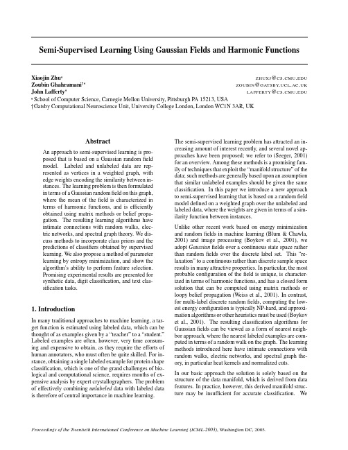
Xiaojin Zhu ZHUXJ@ Zoubin Ghahramani ZOUBIN@ John Lafferty LAFFERTY@ School of Computer Science,Carnegie Mellon University,Pittsburgh PA15213,USAGatsby Computational Neuroscience Unit,University College London,London WC1N3AR,UKAbstractAn approach to semi-supervised learning is pro-posed that is based on a Gaussian randomfieldbeled and unlabeled data are rep-resented as vertices in a weighted graph,withedge weights encoding the similarity between in-stances.The learning problem is then formulatedin terms of a Gaussian randomfield on this graph,where the mean of thefield is characterized interms of harmonic functions,and is efficientlyobtained using matrix methods or belief propa-gation.The resulting learning algorithms haveintimate connections with random walks,elec-tric networks,and spectral graph theory.We dis-cuss methods to incorporate class priors and thepredictions of classifiers obtained by supervisedlearning.We also propose a method of parameterlearning by entropy minimization,and show thealgorithm’s ability to perform feature selection.Promising experimental results are presented forsynthetic data,digit classification,and text clas-sification tasks.1.IntroductionIn many traditional approaches to machine learning,a tar-get function is estimated using labeled data,which can be thought of as examples given by a“teacher”to a“student.”Labeled examples are often,however,very time consum-ing and expensive to obtain,as they require the efforts of human annotators,who must often be quite skilled.For in-stance,obtaining a single labeled example for protein shape classification,which is one of the grand challenges of bio-logical and computational science,requires months of ex-pensive analysis by expert crystallographers.The problem of effectively combining unlabeled data with labeled data is therefore of central importance in machine learning.The semi-supervised learning problem has attracted an in-creasing amount of interest recently,and several novel ap-proaches have been proposed;we refer to(Seeger,2001) for an overview.Among these methods is a promising fam-ily of techniques that exploit the“manifold structure”of the data;such methods are generally based upon an assumption that similar unlabeled examples should be given the same classification.In this paper we introduce a new approach to semi-supervised learning that is based on a randomfield model defined on a weighted graph over the unlabeled and labeled data,where the weights are given in terms of a sim-ilarity function between instances.Unlike other recent work based on energy minimization and randomfields in machine learning(Blum&Chawla, 2001)and image processing(Boykov et al.,2001),we adopt Gaussianfields over a continuous state space rather than randomfields over the discrete label set.This“re-laxation”to a continuous rather than discrete sample space results in many attractive properties.In particular,the most probable configuration of thefield is unique,is character-ized in terms of harmonic functions,and has a closed form solution that can be computed using matrix methods or loopy belief propagation(Weiss et al.,2001).In contrast, for multi-label discrete randomfields,computing the low-est energy configuration is typically NP-hard,and approxi-mation algorithms or other heuristics must be used(Boykov et al.,2001).The resulting classification algorithms for Gaussianfields can be viewed as a form of nearest neigh-bor approach,where the nearest labeled examples are com-puted in terms of a random walk on the graph.The learning methods introduced here have intimate connections with random walks,electric networks,and spectral graph the-ory,in particular heat kernels and normalized cuts.In our basic approach the solution is solely based on the structure of the data manifold,which is derived from data features.In practice,however,this derived manifold struc-ture may be insufficient for accurate classification.WeProceedings of the Twentieth International Conference on Machine Learning(ICML-2003),Washington DC,2003.Figure1.The randomfields used in this work are constructed on labeled and unlabeled examples.We form a graph with weighted edges between instances(in this case scanned digits),with labeled data items appearing as special“boundary”points,and unlabeled points as“interior”points.We consider Gaussian randomfields on this graph.show how the extra evidence of class priors can help classi-fication in Section4.Alternatively,we may combine exter-nal classifiers using vertex weights or“assignment costs,”as described in Section5.Encouraging experimental re-sults for synthetic data,digit classification,and text clas-sification tasks are presented in Section7.One difficulty with the randomfield approach is that the right choice of graph is often not entirely clear,and it may be desirable to learn it from data.In Section6we propose a method for learning these weights by entropy minimization,and show the algorithm’s ability to perform feature selection to better characterize the data manifold.2.Basic FrameworkWe suppose there are labeled points, and unlabeled points;typically. Let be the total number of data points.To be-gin,we assume the labels are binary:.Consider a connected graph with nodes correspond-ing to the data points,with nodes corre-sponding to the labeled points with labels,and nodes corresponding to the unla-beled points.Our task is to assign labels to nodes.We assume an symmetric weight matrix on the edges of the graph is given.For example,when,the weight matrix can be(2)To assign a probability distribution on functions,we form the Gaussianfieldfor(3) which is consistent with our prior notion of smoothness of with respect to the graph.Expressed slightly differently, ,where.Because of the maximum principle of harmonic functions(Doyle&Snell,1984),is unique and is either a constant or it satisfiesfor.To compute the harmonic solution explicitly in terms of matrix operations,we split the weight matrix(and sim-ilarly)into4blocks after the th row and column:(4) Letting where denotes the values on the un-labeled data points,the harmonic solution subject to is given by(5)Figure2.Demonstration of harmonic energy minimization on twosynthetic rge symbols indicate labeled data,otherpoints are unlabeled.In this paper we focus on the above harmonic function as abasis for semi-supervised classification.However,we em-phasize that the Gaussian randomfield model from which this function is derived provides the learning frameworkwith a consistent probabilistic semantics.In the following,we refer to the procedure described aboveas harmonic energy minimization,to underscore the har-monic property(3)as well as the objective function being minimized.Figure2demonstrates the use of harmonic en-ergy minimization on two synthetic datasets.The leftfigure shows that the data has three bands,with,, and;the rightfigure shows two spirals,with,,and.Here we see harmonic energy minimization clearly follows the structure of data, while obviously methods such as kNN would fail to do so.3.Interpretation and ConnectionsAs outlined briefly in this section,the basic framework pre-sented in the previous section can be viewed in several fun-damentally different ways,and these different viewpoints provide a rich and complementary set of techniques for rea-soning about this approach to the semi-supervised learning problem.3.1.Random Walks and Electric NetworksImagine a particle walking along the graph.Starting from an unlabeled node,it moves to a node with proba-bility after one step.The walk continues until the par-ticle hits a labeled node.Then is the probability that the particle,starting from node,hits a labeled node with label1.Here the labeled data is viewed as an“absorbing boundary”for the random walk.This view of the harmonic solution indicates that it is closely related to the random walk approach of Szummer and Jaakkola(2001),however there are two major differ-ences.First,wefix the value of on the labeled points, and second,our solution is an equilibrium state,expressed in terms of a hitting time,while in(Szummer&Jaakkola,2001)the walk crucially depends on the time parameter. We will return to this point when discussing heat kernels. An electrical network interpretation is given in(Doyle& Snell,1984).Imagine the edges of to be resistors with conductance.We connect nodes labeled to a positive voltage source,and points labeled to ground.Thenis the voltage in the resulting electric network on each of the unlabeled nodes.Furthermore minimizes the energy dissipation of the electric network for the given.The harmonic property here follows from Kirchoff’s and Ohm’s laws,and the maximum principle then shows that this is precisely the same solution obtained in(5).3.2.Graph KernelsThe solution can be viewed from the viewpoint of spec-tral graph theory.The heat kernel with time parameter on the graph is defined as.Here is the solution to the heat equation on the graph with initial conditions being a point source at at time.Kondor and Lafferty(2002)propose this as an appropriate kernel for machine learning with categorical data.When used in a kernel method such as a support vector machine,the kernel classifier can be viewed as a solution to the heat equation with initial heat sourceson the labeled data.The time parameter must,however, be chosen using an auxiliary technique,for example cross-validation.Our algorithm uses a different approach which is indepen-dent of,the diffusion time.Let be the lower right submatrix of.Since,it is the Laplacian restricted to the unlabeled nodes in.Consider the heat kernel on this submatrix:.Then describes heat diffusion on the unlabeled subgraph with Dirichlet boundary conditions on the labeled nodes.The Green’s function is the inverse operator of the restricted Laplacian,,which can be expressed in terms of the integral over time of the heat kernel:(6) The harmonic solution(5)can then be written asor(7)Expression(7)shows that this approach can be viewed as a kernel classifier with the kernel and a specific form of kernel machine.(See also(Chung&Yau,2000),where a normalized Laplacian is used instead of the combinatorial Laplacian.)From(6)we also see that the spectrum of is ,where is the spectrum of.This indicates a connection to the work of Chapelle et al.(2002),who ma-nipulate the eigenvalues of the Laplacian to create variouskernels.A related approach is given by Belkin and Niyogi (2002),who propose to regularize functions on by select-ing the top normalized eigenvectors of corresponding to the smallest eigenvalues,thus obtaining the bestfit toin the least squares sense.We remark that ourfits the labeled data exactly,while the order approximation may not.3.3.Spectral Clustering and Graph MincutsThe normalized cut approach of Shi and Malik(2000)has as its objective function the minimization of the Raleigh quotient(8)subject to the constraint.The solution is the second smallest eigenvector of the generalized eigenvalue problem .Yu and Shi(2001)add a grouping bias to the normalized cut to specify which points should be in the same group.Since labeled data can be encoded into such pairwise grouping constraints,this technique can be applied to semi-supervised learning as well.In general, when is close to block diagonal,it can be shown that data points are tightly clustered in the eigenspace spanned by thefirst few eigenvectors of(Ng et al.,2001a;Meila &Shi,2001),leading to various spectral clustering algo-rithms.Perhaps the most interesting and substantial connection to the methods we propose here is the graph mincut approach proposed by Blum and Chawla(2001).The starting point for this work is also a weighted graph,but the semi-supervised learning problem is cast as one offinding a minimum-cut,where negative labeled data is connected (with large weight)to a special source node,and positive labeled data is connected to a special sink node.A mini-mum-cut,which is not necessarily unique,minimizes the objective function,and label0other-wise.We call this rule the harmonic threshold(abbreviated “thresh”below).In terms of the random walk interpreta-tion,ifmakes sense.If there is reason to doubt this assumption,it would be reasonable to attach dongles to labeled nodes as well,and to move the labels to these new nodes.6.Learning the Weight MatrixPreviously we assumed that the weight matrix is given andfixed.In this section,we investigate learning weight functions of the form given by equation(1).We will learn the’s from both labeled and unlabeled data;this will be shown to be useful as a feature selection mechanism which better aligns the graph structure with the data.The usual parameter learning criterion is to maximize the likelihood of labeled data.However,the likelihood crite-rion is not appropriate in this case because the values for labeled data arefixed during training,and moreover likeli-hood doesn’t make sense for the unlabeled data because we do not have a generative model.We propose instead to use average label entropy as a heuristic criterion for parameter learning.The average label entropy of thefield is defined as(13) using the fact that.Both and are sub-matrices of.In the above derivation we use as label probabilities di-rectly;that is,class.If we incorpo-rate class prior information,or combine harmonic energy minimization with other classifiers,it makes sense to min-imize entropy on the combined probabilities.For instance, if we incorporate a class prior using CMN,the probability is given bylabeled set size a c c u r a c yFigure 3.Harmonic energy minimization on digits “1”vs.“2”(left)and on all 10digits (middle)and combining voted-perceptron with harmonic energy minimization on odd vs.even digits (right)Figure 4.Harmonic energy minimization on PC vs.MAC (left),baseball vs.hockey (middle),and MS-Windows vs.MAC (right)10trials.In each trial we randomly sample labeled data from the entire dataset,and use the rest of the images as unlabeled data.If any class is absent from the sampled la-beled set,we redo the sampling.For methods that incorpo-rate class priors ,we estimate from the labeled set with Laplace (“add one”)smoothing.We consider the binary problem of classifying digits “1”vs.“2,”with 1100images in each class.We report aver-age accuracy of the following methods on unlabeled data:thresh,CMN,1NN,and a radial basis function classifier (RBF)which classifies to class 1iff .RBF and 1NN are used simply as baselines.The results are shown in Figure 3.Clearly thresh performs poorly,because the values of are generally close to 1,so the major-ity of examples are classified as digit “1”.This shows the inadequacy of the weight function (1)based on pixel-wise Euclidean distance.However the relative rankings ofare useful,and when coupled with class prior information significantly improved accuracy is obtained.The greatest improvement is achieved by the simple method CMN.We could also have adjusted the decision threshold on thresh’s solution ,so that the class proportion fits the prior .This method is inferior to CMN due to the error in estimating ,and it is not shown in the plot.These same observations are also true for the experiments we performed on several other binary digit classification problems.We also consider the 10-way problem of classifying digits “0”through ’9’.We report the results on a dataset with in-tentionally unbalanced class sizes,with 455,213,129,100,754,970,275,585,166,353examples per class,respec-tively (noting that the results on a balanced dataset are sim-ilar).We report the average accuracy of thresh,CMN,RBF,and 1NN.These methods can handle multi-way classifica-tion directly,or with slight modification in a one-against-all fashion.As the results in Figure 3show,CMN again im-proves performance by incorporating class priors.Next we report the results of document categorization ex-periments using the 20newsgroups dataset.We pick three binary problems:PC (number of documents:982)vs.MAC (961),MS-Windows (958)vs.MAC,and base-ball (994)vs.hockey (999).Each document is minimally processed into a “tf.idf”vector,without applying header re-moval,frequency cutoff,stemming,or a stopword list.Two documents are connected by an edge if is among ’s 10nearest neighbors or if is among ’s 10nearest neigh-bors,as measured by cosine similarity.We use the follow-ing weight function on the edges:(16)We use one-nearest neighbor and the voted perceptron al-gorithm (Freund &Schapire,1999)(10epochs with a lin-ear kernel)as baselines–our results with support vector ma-chines are comparable.The results are shown in Figure 4.As before,each point is the average of10random tri-als.For this data,harmonic energy minimization performsmuch better than the baselines.The improvement from the class prior,however,is less significant.An explanation for why this approach to semi-supervised learning is so effec-tive on the newsgroups data may lie in the common use of quotations within a topic thread:document quotes partof document,quotes part of,and so on.Thus, although documents far apart in the thread may be quite different,they are linked by edges in the graphical repre-sentation of the data,and these links are exploited by the learning algorithm.7.1.Incorporating External ClassifiersWe use the voted-perceptron as our external classifier.For each random trial,we train a voted-perceptron on the la-beled set,and apply it to the unlabeled set.We then use the 0/1hard labels for dongle values,and perform harmonic energy minimization with(10).We use.We evaluate on the artificial but difficult binary problem of classifying odd digits vs.even digits;that is,we group “1,3,5,7,9”and“2,4,6,8,0”into two classes.There are400 images per digit.We use second order polynomial kernel in the voted-perceptron,and train for10epochs.Figure3 shows the results.The accuracy of the voted-perceptron on unlabeled data,averaged over trials,is marked VP in the plot.Independently,we run thresh and CMN.Next we combine thresh with the voted-perceptron,and the result is marked thresh+VP.Finally,we perform class mass nor-malization on the combined result and get CMN+VP.The combination results in higher accuracy than either method alone,suggesting there is complementary information used by each.7.2.Learning the Weight MatrixTo demonstrate the effects of estimating,results on a toy dataset are shown in Figure5.The upper grid is slightly tighter than the lower grid,and they are connected by a few data points.There are two labeled examples,marked with large symbols.We learn the optimal length scales for this dataset by minimizing entropy on unlabeled data.To simplify the problem,wefirst tie the length scales in the two dimensions,so there is only a single parameter to learn.As noted earlier,without smoothing,the entropy approaches the minimum at0as.Under such con-ditions,the results of harmonic energy minimization are usually undesirable,and for this dataset the tighter grid “invades”the sparser one as shown in Figure5(a).With smoothing,the“nuisance minimum”at0gradually disap-pears as the smoothing factor grows,as shown in FigureFigure5.The effect of parameter on harmonic energy mini-mization.(a)If unsmoothed,as,and the algorithm performs poorly.(b)Result at optimal,smoothed with(c)Smoothing helps to remove the entropy minimum. 5(c).When we set,the minimum entropy is0.898 bits at.Harmonic energy minimization under this length scale is shown in Figure5(b),which is able to dis-tinguish the structure of the two grids.If we allow a separate for each dimension,parameter learning is more dramatic.With the same smoothing of ,keeps growing towards infinity(we usefor computation)while stabilizes at0.65, and we reach a minimum entropy of0.619bits.In this case is legitimate;it means that the learning al-gorithm has identified the-direction as irrelevant,based on both the labeled and unlabeled data.Harmonic energy minimization under these parameters gives the same clas-sification as shown in Figure5(b).Next we learn’s for all256dimensions on the“1”vs.“2”digits dataset.For this problem we minimize the entropy with CMN probabilities(15).We randomly pick a split of 92labeled and2108unlabeled examples,and start with all dimensions sharing the same as in previous ex-periments.Then we compute the derivatives of for each dimension separately,and perform gradient descent to min-imize the entropy.The result is shown in Table1.As entropy decreases,the accuracy of CMN and thresh both increase.The learned’s shown in the rightmost plot of Figure6range from181(black)to465(white).A small (black)indicates that the weight is more sensitive to varia-tions in that dimension,while the opposite is true for large (white).We can discern the shapes of a black“1”and a white“2”in thisfigure;that is,the learned parametersCMNstart97.250.73%0.654298.020.39%Table1.Entropy of CMN and accuracies before and after learning ’s on the“1”vs.“2”dataset.Figure6.Learned’s for“1”vs.“2”dataset.From left to right: average“1”,average“2”,initial’s,learned’s.exaggerate variations within class“1”while suppressing variations within class“2”.We have observed that with the default parameters,class“1”has much less variation than class“2”;thus,the learned parameters are,in effect, compensating for the relative tightness of the two classes in feature space.8.ConclusionWe have introduced an approach to semi-supervised learn-ing based on a Gaussian randomfield model defined with respect to a weighted graph representing labeled and unla-beled data.Promising experimental results have been pre-sented for text and digit classification,demonstrating that the framework has the potential to effectively exploit the structure of unlabeled data to improve classification accu-racy.The underlying randomfield gives a coherent proba-bilistic semantics to our approach,but this paper has con-centrated on the use of only the mean of thefield,which is characterized in terms of harmonic functions and spectral graph theory.The fully probabilistic framework is closely related to Gaussian process classification,and this connec-tion suggests principled ways of incorporating class priors and learning hyperparameters;in particular,it is natural to apply evidence maximization or the generalization er-ror bounds that have been studied for Gaussian processes (Seeger,2002).Our work in this direction will be reported in a future publication.ReferencesBelkin,M.,&Niyogi,P.(2002).Using manifold structure for partially labelled classification.Advances in Neural Information Processing Systems,15.Blum,A.,&Chawla,S.(2001).Learning from labeled and unlabeled data using graph mincuts.Proc.18th Interna-tional Conf.on Machine Learning.Boykov,Y.,Veksler,O.,&Zabih,R.(2001).Fast approx-imate energy minimization via graph cuts.IEEE Trans. on Pattern Analysis and Machine Intelligence,23. Chapelle,O.,Weston,J.,&Sch¨o lkopf,B.(2002).Cluster kernels for semi-supervised learning.Advances in Neu-ral Information Processing Systems,15.Chung,F.,&Yau,S.(2000).Discrete Green’s functions. Journal of Combinatorial Theory(A)(pp.191–214). Doyle,P.,&Snell,J.(1984).Random walks and electric networks.Mathematical Assoc.of America. Freund,Y.,&Schapire,R.E.(1999).Large margin classi-fication using the perceptron algorithm.Machine Learn-ing,37(3),277–296.Hull,J.J.(1994).A database for handwritten text recog-nition research.IEEE Transactions on Pattern Analysis and Machine Intelligence,16.Kondor,R.I.,&Lafferty,J.(2002).Diffusion kernels on graphs and other discrete input spaces.Proc.19th Inter-national Conf.on Machine Learning.Le Cun,Y.,Boser, B.,Denker,J.S.,Henderson, D., Howard,R.E.,Howard,W.,&Jackel,L.D.(1990). Handwritten digit recognition with a back-propagation network.Advances in Neural Information Processing Systems,2.Meila,M.,&Shi,J.(2001).A random walks view of spec-tral segmentation.AISTATS.Ng,A.,Jordan,M.,&Weiss,Y.(2001a).On spectral clus-tering:Analysis and an algorithm.Advances in Neural Information Processing Systems,14.Ng,A.Y.,Zheng,A.X.,&Jordan,M.I.(2001b).Link analysis,eigenvectors and stability.International Joint Conference on Artificial Intelligence(IJCAI). Seeger,M.(2001).Learning with labeled and unlabeled data(Technical Report).University of Edinburgh. Seeger,M.(2002).PAC-Bayesian generalization error bounds for Gaussian process classification.Journal of Machine Learning Research,3,233–269.Shi,J.,&Malik,J.(2000).Normalized cuts and image segmentation.IEEE Transactions on Pattern Analysis and Machine Intelligence,22,888–905.Szummer,M.,&Jaakkola,T.(2001).Partially labeled clas-sification with Markov random walks.Advances in Neu-ral Information Processing Systems,14.Weiss,Y.,,&Freeman,W.T.(2001).Correctness of belief propagation in Gaussian graphical models of arbitrary topology.Neural Computation,13,2173–2200.Yu,S.X.,&Shi,J.(2001).Grouping with bias.Advances in Neural Information Processing Systems,14.。


GridRead 读取文件:scheme 方案 journal 日志 profile 外形 Write 保存文件Import :进入另一个运算程序 Interpolate :窜改,插入 Hardcopy : 复制, Batch options 一组选项 Save layout 保存设计Check 检查Info 报告:size 尺寸 ;memory usage 内存使用情况;zones 区域 ;partitions 划分存储区 Polyhedral 多面体:Convert domain 变换范围 Convert skewed cells 变换倾斜的单元 Merge 合并 Separate 分割Fuse (Merge 的意思是将具有相同条件的边界合并成一个;Fuse 将两个网格完全贴合的边界融合成内部(interior)来处理,比如叶轮机中,计算多个叶片时,只需生成一个叶片通道网格,其他通过复制后,将重合的周期边界Fuse 掉就行了。
注意两个命令均为不可逆操作,在进行操作时注意保存case)Zone 区域: append case file 添加case 文档 Replace 取代;delete 删除;deactivate 使复位;Surface mesh 表面网孔Reordr 追加,添加:Domain 范围;zones 区域; Print bandwidth 打印 Scale 单位变换 Translate 转化Rotate 旋转 smooth/swap 光滑/交换Models 模型:solver 解算器Pressure based 基于压力density based 基于密度implicit 隐式,explicit 显示Space 空间:2D,axisymmetric(转动轴),axisymmetric swirl (漩涡转动轴);Time时间:steady 定常,unsteady 非定常Velocity formulation 制定速度:absolute绝对的;relative 相对的Gradient option 梯度选择:以单元作基础;以节点作基础;以单元作梯度的最小正方形。

外文原文Stages of Corporate CitizenshipBusiness leaders throughout the world are making corporate citizenship a key priority for their companies.1 Some are updating policies and revising programs; others are forming citizenship steering committees, measuring their environmental and social performance, and issuing public reports. Select firms are striving to align staff functions responsible for citizenship and move responsibility—and accountability—into lines of business. Vanguard companies are trying to create a broader market for citizenship and offer products and services that aim explicitly to both make money and make a better world.Amid the flurry of activity, many executives wonder what’s going on and worry whether or not their myriad citizenship initiatives make sense. Is their company prepared to take appropriate and effective actions on transparency, governance, community economic development, work-family balance, environmental sustainability, human rights protection, and ethical investor relationships?Is there any connection between, say, efforts in risk management, corporate branding, stakeholder engagement, supplier certification, cause related marketing, and employee diversity? Should there be? Studies conducted by the Center for Corporate Citizenship at Boston College suggest that the balance between confusion and coherence depends very much on what stage a company is in its development of corporate citizenship.Comparative neophytes, for instance, often lack understanding of these many aspects of corporate citizenship and have neither the expertise nor the machinery to respond to so many diverse interests and demands. Their chief challenges are to put citizenship firmly on the corporate agenda, get better informed about stakeholders’ concerns, and take some sensible initial steps.At the other extreme are companies that have already made a full-blown foray into citizenship. Their CEO is typically leading the firm’s position on social and environmental issues, and their Board is fully informed about company practices. Should these firms want to move forward, they might next try to connect citizenship to corporate branding and everyday employees through a “live the brand” campaign like those at IBM and Novo Nordisk or establish citizenship objectives for line managers, as DuPont and UBS have done.When it comes to making sense of corporate citizenship, much depends on what acompany has accomplished to date and how far it wants (and has to) go. The Center’s surveys of a random sample of American businesses find that roughly ten percent of company leaders don’t understand what corporate citizenship is all about. On the other end of the spectrum, not quite as many firms have integrated programs and are setting new standards of performance. In the vast majority in between, there is a wide range of companies in transition whose knowledge, attitudes, structures, and practices represent different degrees of understanding of and sophistication about corporate citizenship.Knowing at what stage a company is, and what challenges it faces in advancing citizenship, can clear up an executive’s confusion about where things stand, frame strategic choices about where to go, aid in setting benchmarks and goals, and perhaps speed movement forward.Stages of DevelopmentWhat does it mean that a company is at a “stage” of corporate citizenship?The general idea—found in the study of children, groups, and systems of all types, including business organizations—is that there are distinct patterns of activity at different points of development. Typically, these activities become more complex and sophisticated as development progresses and therefore capacities to respond to environmental challenges increase in kind. Piaget’s developmental theory, for example, has children progress through stages that entail more complex thinking and finer judgments about how to negotiate the social world outside of themselves. Similarly, groups mature along a developmental path as they confront emotional and task challenges that require more socially sensitive interaction and sophisticated problem solving.Greiner, in his groundbreaking study of organizational growth, found that companies also develop more complex ways of doing things at different stages of growth. They must, over time, find more direction after their creative start-up phase, develop an infrastructure and systems to take on more responsibilities, and then “work through” the challenges of over-control and red-tape through coordination and later collaboration across work units and levels.Development of CitizenshipThere are a number of models of “stages” of corporate citizenship. On a macro scale, for example, scholars have tracked changing conceptions of the role of business in society as advanced by business leaders, governments, academics, and multi-sectorassociations. They document how increasingly elaborate and inclusive definitions of social responsibility, environmental protection, and corporate ethics and governance have developed over recent decades that enlarge the role of business in society. Others have looked into the spread of these ideas into industry and society in the form of social and professional movements.At the level of the firm, Post and Altman have shown how environmental policies progressively broaden and deepen as companies encounter more demanding expectations and build their capability to meet them. In turn, Zadek’s case study of Nike’s response to challenges in its supply chain highlights stages in the development of attitudes about social responsibilities in companies and in corporate responsiveness to social issues. Both of these studies emphasize the role of organizational learning as conceptions of company responsibilities become more complex at successive stages of development, action requirements are more demanding, and the organizational structures, processes, and systems used to manage citizenship are more elaborate and comprehensive.What such firm-level frameworks have not fully addressed are the generative logic and mechanisms that drive the development of citizenship within organizations. Here we consider the development of citizenship as a stage-by-stage process where a combination of internal capabilities applied to environmental challenges propels development forward in a m ore or less “normal” or normative logic.Greiner’s model of organizational growth illustrates this normative trajectory. In his terms, the development of an organization is punctuated by a series of predictable crises that trigger responses that move the organization forward. What are the triggering mechanisms? They are tensions between current practices and the problems they produce that demand a new response from a firm. For instance, creativity, the entrepreneurial fire in companies in their first stage, also generates confusion and a loss of focus that can stall growth. This poses a “crisis of leadership” that is resolved—and a stage of orderly growth results—once the firm gains direction, often under new leadership and with more formal structures. A later tension between delegation and its consequences, sub-optimization and inter-group conflict, triggers a “crisis of control” and moves toward coordination. In development language, companies in effect “master” these challenges by devising progressively more effective and elaborate responses to them.The model presented here is also normative in that it posits a series of stages in thedevelopment of corporate citizenship. The triggers for movement are challenges that call for a fresh response. These challenges center initially on a firm’s credibility as a corporate citizen, then its capacities to meet expectations, the coherence of its many subsequent efforts, and, finally, its commitment to institutionalize citizenship in its business strategies and culture.Movement along a single development path is not fixed nor is attaining a penultimate “end state” a logical conclusion. This means that the arc of citizenship within any particular firm is shaped by the socio-economic, environmental, and institutional forces impinging on the enterprise. This effect is well documented by Vogel’s analysis of the “market for virtue” where he finds considerable variability in the business case for citizenship across firms and industries and thus limits to its marketp lace rewards. Notwithstanding, a company’s response to these market forces also varies based on the attitudes and outlooks of its leaders, the design and management of its citizenship agenda, and firmspecific learning. Thus, there are “companies with a conscience” that have a more expansive citizenship profile and firms that create a market for their good works.Dimensions of CitizenshipTo track the developmental path of citizenship in companies, we focus on seven dimensions of citizenship that vary at each stage:Citizenship Concept: How is citizenship defined? How comprehensive is it? Definitions of corporate citizenship are many and varied. The Center’s concept of citizenship considers the total actions of a corporation (commercial and philanthropic). Bettignies makes the point that terms such as citizenship and sustainability incorporate notions of ethics, philanthropy, stakeholder management, and social and environmental responsibilities into an integrative framework that guides corporate action.Strategic Intent: What is the purpose of citizenship in a company? What it is trying to achieve through citizenship? Smith observes that few companies embrace a strictly moral commitment to citizenship; instead most consider specific reputational risks and benefits in the market and society and thereby establish a business case for their efforts. Rochlin and Googins, in turn,see increasing interest in an “inside-out” framing where a value proposition for citizenship guides actions and investments. Leadership: Do top leaders support citizenship? Do they lead the effort? Visible, active, top level leadership appears on every survey as the number one factor drivingcitizenship in a corporation. How well informed are top leaders are about citizenship, how much leadership do they exercise, and to what extent do they “walk the talk”? Structure: How are responsibilities for citizenship managed? A three-year indepth study of eight companies in the Center’s Executive Forum on Corporate Citizenship found that many progressed from managing citizenship from functional “islands” to cross-functional committees and that a few had begun to achieve more formal integration through a combination of structures, processes, and systems.Issues Management: How does a company deal with citizenship issues that arise? Scholars have mapped the evolution of the public affairs office in corporations and stages in the management of public issues. How responsive a company is in terms of citizenship policies, programs, and performance?Stakeholder Relationships: How does a company engage its stakeholders? A wide range of trends—from increased social activism by shareholders to an increase in the number of non-governmental organizations (NGOs) around the world—has driven major changes in the ways companies communicate with and engage their stakeholders.Transparency: How “open” is a company about its financial, social, and environmental performance? The web sites of upwards of 80% of Fortune 500 companies address social and environmental issues and roughly half of the companies today issue a public report on their activities.Citizenship at Each StageThe model in Figure 1 presents the stages in the development of corporate citizenship along these seven dimensions. We illustrate each stage with selected examples of corporate practice. (Note, however, that we are not implying that these companies currently operate at that stage; rather, at the times noted, they were illustrative of citizenship at that development stage.) A close inspection of these companies reveals instances where they had a leading-edge practice in some dimensions but were less developed in others. This should come as no surprise. For example, the pace of a child’s physical, mental, and emotional development is seldom uniform. One facet typically develops faster than another. In the same way, the development of group and organizational capabilities is uneven. Firm-specific forces in society, industry dynamics, and other environmental influences feature in how citizenship develops within a firm.Stage 1. ElementaryAt this base stage, citizenship activity in a company is episodic and its programs are undeveloped. The reasons are straightforward: scant awareness of what corporate citizenship is all about, uninterested or indifferent top management, and limited or one-way interactions with external stakeholders, particularly in the social and environmental sectors. The mindset in these companies, and associated policies and practices, often centers on simple compliance with laws and industry standards.Responsibilities for handling matters of compliance in these firms are usually assigned to the functional heads of human resources, the legal department, investor relations, public relations, and community affairs. The job of these functional managers is to make sure that the company obeys the law and to keep problems that might arise from harming the firm’s reputation. In many cases, they take a defensive stance toward outside pressures—e.g., Nike’s dealings with labor activists in the early 1990s.Some corporate leaders, for example, have espoused economist Milton Friedman’s notion that their company’s obligations to society are solely to“make a profit, pay taxes, and provide jobs.”20 Others, particularly those heading smaller and mid-size businesses, comply willingly with employment and health, safety, and environmental regulations but have neither the resources nor the wherewithal to do much more for their employees, communities, or society.Former General Electric CEO Jack Welch is an exemplar of this principled big-business view. “A CEO’s primary social responsibility is to assure the financial success of the company,” he says. “Only a healthy, winning company has the resources and capability to do the right thing.”21GE’s financial success over the past two decades is unquestioned. However, the company’s reputation suffered toward the end of Welch’s tenure when it was revealed that that one of its business units had discharged tons of the toxic chemical PCB into the Hudson River. When challenged, Welch was defensive and pointed out that GE had fully complied with then existing environmental protection laws.This illustrates one of the triggers that move a company forward into a new stage of citizenship. Welch’s sta nce was plainly out of touch with changing expectations of corporate responsibilities and the contradiction between GE’s success at wealth creation and loss of reputation was palpable. Welch’s successor,Jeffrey Immelt, reversed this course, accepted at least partial financial responsibility for the clean up, and thereafter reprioritized citizenship on the company’s agenda.中文译文企业公民的阶段全世界的商界领袖都认为企业公民是他们公司的一个优先环节。
fluent 操作界面中英文对照Read 读取文件:scheme 方案journal 日志profile 外形 Write 保存文件Import :进入另一个运算程序 Interpolate :窜改,插入 Hardcopy : 复制, Batch options 一组选项 Save layout 保存设计Grid 网格Check 检查Info 报告:size 尺寸 ;memory usage 内存使用 情况;zones 区域;partitions 划分存储区 Polyhedral 多面体:Convert domain 变换范围Convert skewed cells 变换倾斜的单元Merge 合并 Separate 分割Fuse (Merge 的意思是将具有相同条件的边界合 并成一个;Fuse 将两个网格完全贴合的边界融合 成内部(interior)来处理,比如叶轮机中,计算多 个叶片时,只需生成一个叶片通道网格,其他通 过复制后,将重合的周期边界Fuse 掉就行了。
注意两个命令均为不可逆操作,在进行操作时注 意保存case) Zone 区域: append case file 添力口 case 文档 Replace 取代;delete 删除;deactivate 使复 位; Surface mesh 表面网孔Reordr 追加,添加:Domain 范围;zones 区域; Print bandwidth 打印 Scale 单位变换 Translate 转化Rotate 旋转 smooth/swap 光滑/交换CheckInfo ► Polyhedra►Merge...Separate ► Fuse...Zone►Surface Mesh... Reorder►Scale...Translate...Rotate...Smooth/Swap...ieGrid ] Define Solvea:w 1E3 SolverSolver* Pressure Based 'Density Based Space「2DL Axisymmetric 广 Axcsymmetric Swirl m 3DVelgty Formulatiqn • Absolute RelativeGradient Option区 Implicit「Explicit Time# SteadyUnsteadyPorous Formulation• Superficial VelocityPhysical Veiccity6K | Cancel] Help |Pressure based 基于压力 Density based 基于密度Models 模型:solver 解算器Formulation # Green-Gauss Cell Oased Green-Gauss N 。
Learning to Detect a Salient ObjectTie Liu,Zejian Yuan,Jian Sun,Jingdong Wang,Nanning Zheng,Fellow,IEEE, Xiaoou Tang,Fellow,IEEE,and Heung-Yeung Shum,Fellow,IEEE Abstract—In this paper,we study the salient object detection problem for images.We formulate this problem as a binary labeling task where we separate the salient object from the background.We propose a set of novel features,including multiscale contrast,center-surround histogram,and color spatial distribution,to describe a salient object locally,regionally,and globally.A conditional random field is learned to effectively combine these features for salient object detection.Further,we extend the proposed approach to detect a salient object from sequential images by introducing the dynamic salient features.We collected a large image database containing tens of thousands of carefully labeled images by multiple users and a video segment database,and conducted a set of experiments over them to demonstrate the effectiveness of the proposed approach.Index Terms—Salient object detection,conditional random field,visual attention,saliency map.Ç1I NTRODUCTIONT HE human brain and visual system pay more attention to some parts of an image.Visual attention has been studied by researchers in physiology,psychology,neural systems,and computer vision for a long time.There are many applications for visual attention,for example,auto-matic image cropping[1],adaptive image display on small devices[2],image/video compression,advertising design [3],and image collection browsing[4].Recent studies[5], [6],[7]demonstrated that visual attention helps object recognition,tracking,and detection as well.In this paper, we study one aspect of visual attention—salient object detection.Fig.1shows some examples of salient objects.For instance,people are usually interested in the objects in images in Fig.1,and the leaf,car,and woman attract the most visual attention in each respective image.We call them salient objects or foreground objects that we are familiar with,or objects with the most interest.In many applica-tions,such as image display on small devices[2]and image collection browsing[4],people want to show the regions with the most interest,or the salient objects.In this paper, we try to locate these salient objects automatically with the supposition that a salient object exists in an image.1.1Related WorkMost existing visual attention approaches are based on the bottom-up computational framework[8],[9],[10],[11],[12], [13],[14],[15],[16],where visual attention is supposed to be driven by low-level stimulus in the scene,such as intensity, contrast,and motion.These approaches consist of the following three steps:The first step is feature extraction in which multiple low-level visual features,such as intensity, color,orientation,texture,and motion,are extracted from the image at multiple scales.The second step is saliency computation.The saliency is computed by a center-surround operation[13],self-information[8],or graph-based random walk[9]using multiple features.After normalization and linear/nonlinear combination,a master map[17]or a saliency map[14]is computed to represent the saliency of each image st,a few key locations on the saliency map are identified by winner-take-all,or inhibition-of-return,or other nonlinear operations.Recently,a saliency model based on low,middle,and high-level image features was trained using the collected eye tracking data[18].While these approaches have worked well in finding a few fixation locations in synthetic and natural images,they have not been able to accurately detect where the salient object should be.For instance,the middle row in Fig.1shows three saliency maps computed using Itti’s algorithm[13].Note that the visual saliency concentrates on several small local regions with high-contrast structures,e.g.,the background grid in Fig.1a,the shadow in Fig.1b,and the foreground boundary in Fig.1c.Although the leaf in Fig.1a commands much attention,the saliency for the leaf is low.Therefore, these saliency maps computed from low-level features don’t have the notation of objects,and they are not good indications for where a salient object is located while perusing these images.Figure-ground segregation is somehow related to salient object detection.However,the usually figure-ground.T.Liu is with the Institute of Artificial Intelligence and Robotics,Xi’anJiaotong University,and the Analytics and Optimization Department,IBM Research-China,Building19A2F,Zhongguancun Software Park,8Dongbeiwang West Road,Haidian District,Beijing100193,P.R.China.E-mail:liultie@..Z.Yuan and N.Zheng are with the Institute of Artificial Intelligence andRobotics,Xi’an Jiaotong University,28Xianning Xilu,Xi’an710049,China.E-mail:yzejian@,nnzheng@..J.Sun is with the Visual Computing Group,Microsoft Research Asia,5/F,Beijing Sigma Center,No.49,Zhichun Road,Haidian District,Beijing100190,P.R.China.E-mail:jiansun@..J.Wang is with the Media Computing Group,Microsoft Research Asia,5/F,Beijing Sigma Center,No.49,Zhichun Road,Haidian District,Beijing100190,P.R.China.E-mail:jingdw@..X.Tang is with the Department of Information Engineering,ChineseUniversity of Hong Kong,Shatin,Hong Kong.E-mail:xtang@.hk..H.-Y.Shum is with the On-Line Service Division,R&D,Microsoft,OneMicrosoft Way,Redmond,WA98052.E-mail:hshum@.Manuscript received4Dec.2008;revised23Oct.2009;accepted29Nov.2009;published online2Mar.2010.Recommended for acceptance by A.Torralba.For information on obtaining reprints of this article,please send e-mail to:tpami@,and reference IEEECS Log NumberTPAMI-2008-12-0834.Digital Object Identifier no.10.1109/TPAMI.2010.70.0162-8828/11/$26.00ß2011IEEE Published by the IEEE Computer Societysegregation algorithm works with the supposition of the category of objects [19],[20],[21]or with interactions [22],[23].If the object is assigned a given category,the specific features,for example,for cows,can be defined specially,and these features cannot be adopted for other categories.For interactive figure-ground segmentation,the appearance model is usually set up,where for our salient object detection,we do not have such an appearance model.Visual attention is also studied for sequential images,where the spatiotemporal cues from image sequences are indicated to be helpful for visual attention detection.For instance,motion from objects or backgrounds helps to indicate the salient fixations [24],[25],[26].Large motion [27]and motion contract [24]are supposed to induce prominent attention,ually,the visual saliency from a single image is combined with the motion saliency for better visual attention detection,and different combination strate-gies are introduced in [27].Video surprising [11]is also related,where it describes the KullbackLeibler divergence between the prior and posterior distribution of a feature map.These visual attention approaches suffer from the similar shortcoming to the visual attention approaches for single image.Automatic object discovery [28],[29],[30]deals with a similar salient object detection task for sequential images.The objects are extracted and tracked using motion-based layer segmentation in [28]and a generative model of objects by defining switch variables for combinatorial model selection is adopted in [29].The unsupervised video object discovery [30]combines the topic model and the temporal model for videos.1.2Our ApproachIn this paper,we investigate one aspect of visual attention,namely,salient object detection.We incorporate the high-level concept of the salient object into the process of saliency map computation.As can be observed in Fig.2,people naturally pay more attention to salient objects in images,such as a person,a face,a car,an animal,or a road sign.Therefore,we formulate salient object detection as a binary labeling problem that separates a salient object from thebackground.Like face detection,we learn to detect a familiar object;unlike face detection,we detect a familiar yet unknown object in an image.We present a supervised approach to learn to detect a salient object in an image or sequential images.First,we model the salient object detection problem by a condition random field (CRF),where a group of salient features are combined through CRF learning.Moreover,the segmenta-tion is also incorporated into the CRF to detect a salient object with unknown size and shape.The last row in Fig.1shows the saliency maps computed by our approach.Second,to overcome the challenge that we do not know what a specific object or object category is,we propose a set of novel local,regional,and global salient features to define a generic salient object.We also define the salient features on the motion field similarly to capture the spatiotemporal cues.Then,we construct a large image database with 20,000+well-labeled images for training and evaluation.To the best of our knowledge,it is the first time a large image database has been made available for quantitative evaluation.The remainder of the paper is organized as follows:Section 2introduces the formulation of the salient object detection problem,and the salient object features are presented in Section 3.Section 4introduces the image database and the evaluation experiments.Section 5dis-cusses the connections between our approach and related approaches,and the conclusion follows in Section 6.2F ORMULATIONGiven an image I ,we represent the salient object as a binary mask A ¼f a x g .For each pixel x ,a x 2f 1;0g is a binary label to indicate whether the pixel x belongs to the salient object.Similarly,the salient objects in sequential images,f I 1;...;I t ;...;I N g ,are represented by a sequence of binary masks f A 1;...;A t ;...;A N g ,with A t corresponding to image I t .In this paper,we formulate the salient object detection problem as a binary labeling task by inspecting whether each pixel belongs to the salient object.We first present the conditional random field formulation to the single-imageFig. 2.Sample images in our image database for salient objectdetection.Fig.1.Salient object detection.From top to bottom:input image with a salient object,saliency map computed by Itti’s attention algorithm (),and saliency map computed by our salient object detection approach.case,and then extend it to the sequential image case by exploring the extra temporal information.2.1Formulation of Salient Object Detection in aSingle ImageIn the CRF framework[31],the probability of a labeling configuration A¼f a x g,given the observation image I, is modeled as a conditional distribution PðA j IÞ¼1 Z expðÀEðA j IÞÞ,where Z is the partition function.Wedefine the energy EðA j IÞas a linear combination of a set of static salient features,including a number of K unary features F kða x;IÞand a pairwise feature Sða x;a x0;IÞ:EðA j IÞ¼Xx X Kk¼1k F kða x;IÞþXx;x0Sða x;a x0;IÞ;ð1Þwhere k is the weight of the k th feature and x;x0are two adjacent pared with Markov random field,one of the advantages of CRF is that the features F kða x;IÞand Sða x;a x0;IÞcan be arbitrary low-level or high-level features extracted from the whole image.CRF also provides an elegant framework to learn an optimal combination of multiple features.Salient object feature.F kða x;IÞindicates whether a pixel x belongs to the salient object.In the next section,we propose a set of local,regional,and global salient object features.The salient object feature F kða x;IÞis formulated from a normalized feature map f kðx;IÞ2½0;1 for every pixel,and is written as follows:F kða x;IÞ¼f kðx;IÞ;a x¼0;1Àf kðx;IÞ;a x¼1:&ð2ÞPairwise feature.Sða x;a x0;IÞexploits the spatial rela-tionship between two adjacent pixels.Following the contrast-sensitive potential function in interactive image segmentation[22],we define Sða x;a x0;IÞasSða x;a x0;IÞ¼j a xÀa x0jÁexpðÀ d x;x0Þ;ð3Þwhere d x;x0¼k I xÀI x0k2is the L2-norm of the color differ-ence, is a robust parameter that weights the color contrast and can be set as ¼ð2hk I xÀI x0k2iÞÀ1[32],with hÁi being the expectation operator.This feature function can be viewed as a penalty term when adjacent pixels are assigned with different labels.The more similar the colors of the two pixels are,the less likely it is that they are assigned different labels.2.2Formulation of Salient Object Detection inSequential ImagesWe exploit the extra temporal cues to formulate salient object detection in sequential images.Besides the static salient features from a single image,the temporal features,called dynamic features,are further defined.Differently from previous work[24],[25],[26],we propose new dynamic features and learn a CRF model to combine the dynamic features and static features.Instead of building a complex3D graph formulation,e.g.,a large graph in interactive video cutout[33],[34],we integrate the cues from multiple images into a2D graph for effective and efficient optimization.Given the sequential images f I t g,t2f1;...;N g,the probability of the sequential binary maps,f A t g, t2f1;...;N g,can be modeled as a conditional distribution:PðA1;...;N j I1;...;NÞ¼1ZexpðÀEðA1;...;N j I1;...;NÞÞ;ð4Þwhere Z is the partition function.A reasonable supposition is that the salient object detection A t can be inferred from the associated frame I t and the previous frame I tÀ1.Then, the energy function EðA1;...;N j I1;...;NÞcan be decomposed as EðA1;...;N j I1;...;NÞ¼X Nt¼1EðA t j I1;...;NÞ¼X Nt¼1EðA t j I tÀ1;I tÞ:ð5ÞHere,EðA t j I tÀ1;I tÞis composed of a static term and a dynamic term.The static term is the same as the single-image case.In the dynamic term,we compute a motion field M t from a pair of successive images I tÀ1and I t,and build salient features from the motion field,and in addition, introduce an appearance coherent feature between the salient objects in the successive frames.Specifically,the energy EðA t j I tÀ1;I tÞis formulated as a linear combination of static salient features F kða x;I tÞ,a pairwise feature Sða x;a x0;IÞ,and a set of dynamic salient features,including motion salient features F kða x;M tÞand appearance coherent features F kða x;I tÀ1;I tÞ:EðA t j I tÀ1;I tÞ¼XxX Kk¼1k F kða x;I tÞþXKþLk¼Kþ1k F kða x;M tÞþ 0Fða x;I tÀ1;I tÞ!þXx;x0Sða x;a x0;I tÞ;ð6Þwhere f k g are the weights of the features,M t is the motion field corresponding to image I t,and x;x0are two adjacent pixels in image I t.F kða x;I tÞare the static salient features,and Sða x;a x0;I tÞdescribes the spatial relationship between two adjacent pixels.These two categories of features are defined as in(1).Differently from(1),more features from the temporal information are included.These are the motion salient features F kða x;M tÞfrom the motion field M t and the appearance coherent feature Fða x;I tÀ1;I tÞbetween the salient objects from two adjacent frames.Motion salient feature.F kða x;M tÞis defined,similarly to(2),as the indicator of a normalized feature mapf kðx;M tÞ2½0;1 ,where M t is the motion field of the image I t and obtained based on the SIFT flow technique[35].Appearance coherent feature.Fða x;I tÀ1;I tÞmodels the appearance coherence of the salient objects from two adjacent frames,which is defined as an indicator of a normalized feature map fðx;I tÀ1;I tÞ2½0;1 ,similarly to(2). This feature function fðx;I tÀ1;I tÞpenalizes the pixels that are identified to be in the salient object,but with a large color difference between the surrounding regions from two adjacent frames.With this appearance coherent feature,the salient objects from two adjacent frames can be labeled more consistently.2.3Learning and Inference for The CRF ModelThe objective functions of the salient object detection for single-image and sequential-image cases in(1)and(6)are essentially very similar to the perspective of the CRF formulation,i.e.,a linear combination of a set of features.To get the linear combination of features,the goal of CRFLIU ET AL.:LEARNING TO DETECT A SALIENT OBJECT355learning is to estimate the linear weights !¼f k g under the Maximized Likelihood (ML)criteria.In the following,we present the parameter learning scheme for the single-image case.The parameter learning scheme for the sequential image case can be similarly obtained.Given N training image pairs f I n ;A n g N n ¼1,the optimal parameters maximize the sum of the log-likelihood:Ã!¼arg max !X n log P ðA n j I n ; !Þ:ð7ÞThe derivative of the log-likelihood with respect to the parameter k is the difference between two expectations:d log P ðA n j I n ; !Þd k¼<F k ðA n ;I n Þ>P ðA n j I n ; !ÞÀ<F k ðA n ;I n Þ>P ðA n j G n Þ:ð8ÞThen,the gradient descent direction isÁ k /X nX x;a n xÀF k Àa n x ;I nÁp Àa n x j I n ;!ÁÀF k Àa n x ;I n Áp Àa n x j g n xÁÁ;ð9Þwhere p ða n x j I n ; !Þ¼R A n n a n xP ðA n x j I n ; !Þis the marginal dis-tribution and p ða n x j g n x Þis from the labeled ground truth g n x andis defined asp Àa n x j g n x Á¼1Àg n x ;a x ¼0;g nx ;a x ¼1:&ð10ÞExact computation of marginal distribution p ða n x j I n ; !Þisintractable.However,the pseudomarginal (belief)com-puted by belief propagation can be used as a good approximation [36],[19].The tree-reweighted belief propa-gation [37]can be run under the current parameters in each step of gradient descent to compute an approximation ofthe marginal distribution p ða n xj I n ; !Þ.When the combination parameters of salient features are learned,we can infer the most probable labeling A to minimize the energy from (1)and (6).We still apply the tree-reweighted belief propagation to infer the label using the learned parameters,and we will discuss the details of implementations in Section 4.3S ALIENT O BJECT F EATUREIn this section,we instantiate the formulation of salient object detection by presenting the salient object features:static salient features for the single-image case and dynamic salient features specifically for the sequential images.3.1Static Salient FeatureWe introduce local,regional,and global features that define a salient object.Since the scale selection is one of the fundamental issues in feature extraction,we resize all images so that the max(width,height)of the image is 400pixels.In the following,all parameters are set with respect to this basic image size.3.1.1Multiscale ContrastContrast is the most commonly used local feature for attention detection [13],[38],[39]because the contrast operator simulates the human visual receptive fields.With-out knowing the size of the salient object,contrast is usually computed at multiple scales.In this paper,we simply define the multiscale contrast feature f c ðx;I Þas a linear combina-tion of contrasts in the Gaussian image pyramid:f c ðx;I Þ¼X L l ¼1X x 02N ðx Þk I l ðx ÞÀI l ðx 0Þk 2;ð11Þwhere I l is the l th-level image in the pyramid and the number of pyramid levels L is 6.N ðx Þis a 9Â9window.The feature map f c ðÁ;I Þis normalized to a fixed range ½0;1 .An example is shown in Fig. 3.Multiscale contrast highlights the high-contrast boundaries by giving low scores to the homogenous regions inside the salient object.3.1.2Center-Surround HistogramAs shown in Fig.2,the salient object usually has a larger extent than local contrast and can be distinguished from its surrounding context.Therefore,we propose a regional salient feature.Suppose the salient object is enclosed by a rectangle R .We construct a surrounding contour R S with the same area of R ,as shown in Fig.4a.To measure how distinct the salient object in the rectangle is with respect to its surroundings,we can measure the distance between R and R S using various visual cues such as intensity,color,and texture/texton.In this paper,we use the 2distance between histograms ofRGB color: 2ðR;R S Þ¼12P ðR i ÀR i S Þ2i iS.We use histograms because they are a robust global description of appearance.They are insensitive to small changes in size,shape,and viewpoint.Another reason is that the histogram of a rectangle with any location and size can be very quickly computed by means of an integral histogram introduced recently [40].Fig.4a shows that the salient object (the girl)is most distinct using the 2histogram distance.We have also tried the intensity histograms and histograms of oriented gradient [41].We found that the former is redundant with the color histogram and the latter is not a good measurement because the texture distribution in a semantic object is usually not coherent.To handle varying aspect ratios of the object,we use five templates with different aspect ratios f 0:5;0:75;1:0,1:5;2:0g .356IEEE TRANSACTIONS ON PATTERN ANALYSIS AND MACHINE INTELLIGENCE,VOL.33,NO.2,FEBRUARY2011Fig.3.Multiscale contrast.From left to right:input image,contrast maps at multiple scales,and the feature map from linearly combining the contrasts at multiple scales.We find the most distinct rectangle,R Ãðx Þ,centered at each pixel x by varying the size and aspect ratio:R Ãðx Þ¼arg max R ðx Þ2ðR ðx Þ;R S ðx ÞÞ:ð12ÞThe size range of the rectangle R ðx Þis set to ½0:1;0:7 Âmin ðw;h Þ,where w;h are the image width and height.Then,the center-surround histogram feature f h ðx;I Þis defined as a sum of spatially weighted distances:f h ðx;I Þ/Xf x 0j x 2R Ãðx 0Þgw xx 0 2ðR Ãðx 0Þ;R ÃS ðx 0ÞÞ;ð13Þwhere R Ãðx 0Þis the rectangle centered at x 0and containingthe pixel x .The weight w xx 0¼exp ðÀ0:5 À2x 0k x Àx 0k 2Þis a Gaussian falloff weight with variance 2x 0,which is set to one-third of the size of R Ãðx 0Þ.Finally,the feature map f h ðÁ;I Þis also normalized to the range ½0;1 .Fig.4b shows several center-surround feature maps.The salient objects are well located by the center-surround histogram feature.The last image in Fig.4b is an especially difficult case for color or contrast-based approaches but the center-surround histogram feature can capture the “object-level”salient region.To further verify the effectiveness of this feature,we compare the center-surround histogram distance of a randomly selected rectangle,a rectangle centered at the image center,and three user-labeled rectangles in the image.Fig.5shows the average distances on the image set A ,and this image set is introduced in Section 4.It is no surprise that the salient object has a large center-surround histogram distance.3.1.3Color Spatial DistributionThe center-surround histogram is a regional feature.Is there a global feature related to the salient object?We observe from Fig.2that the more widely a color is distributed in the image,the less possible it is that a salient object contains this color.The global spatial distribution of a specific color can be used to describe the saliency of an object.To describe the spatial distribution of a specific color,the simplest approach is to compute the spatial variance of the color.First,all colors in the image are represented by Gaussian Mixture Models (GMMs)f w c ; c ;Æc g C c ¼1,where f w c ; c ;Æc g is the weight,the mean color,and the covar-iance matrix of the c th component.Each pixel is assigned to a color component with the probability:p ðc j I x Þ¼w c N ðI x j c ;Æc ÞPcw c N ðI x j c ;Æc Þ:ð14ÞThen,the horizontal variance V h ðc Þof the spatial positionfor each color component c isV h ðc Þ¼1c Xxp ðc j I x ÞÁj x h ÀM h ðc Þj 2;ð15ÞM h ðc Þ¼1j X j c Xxp ðc j I x ÞÁx h ;ð16Þwhere x h is the x-coordinate of the pixel x andj X j c ¼Px p ðc j I x Þ.The vertical variance V v ðc Þis similarly defined.The spatial variance of a component c is V ðc Þ¼V h ðc ÞþV v ðc Þ.We normalized f V ðc Þg c to the range ½0;1 (V ðc Þ ðV ðc ÞÀmin c V ðc ÞÞ=ðmax c V ðc ÞÀmin c V ðc ÞÞ).Finally,the color spatial-distribution feature f s ðx;I Þis defined as a weighted sum:f s ðx;I Þ/Xcp ðc j I x ÞÁð1ÀV ðc ÞÞ:ð17ÞThe feature map f s ðÁ;I Þis also normalized to the range ½0;1 .Fig.6b shows color spatial-distribution feature maps of several example images.The salient objects are well covered by this global feature.Note that the spatial variance of the color at the image corners or boundaries may also be small because the image is cropped from the whole scene.To reduce this artifact,a center-weighted,spatial-variance feature is defined asLIUET AL.:LEARNING TO DETECT A SALIENT OBJECT 357Fig.5.The average center-surround histogram distance on the image set A .1.A randomly selected rectangle.2.A rectangle centered at the image center with 55percent ratioof area to image.3-5.Rectangles labeled by three users.Fig. 4.Center-surround histogram.(a)Center-surround histogram distances with different locations and sizes.(b)Top row are input images and bottom row are center-surround histogram feature maps.f s ðx;I Þ/X cp ðc j I x ÞÁð1ÀV ðc ÞÞÁð1ÀD ðc ÞÞ;ð18Þwhere D ðc Þ¼Px p ðc j I x Þd x is the weight which assigns less importance to colors nearby image boundaries and is also normalized to ½0;1 ,similarly to V ðc Þ.d x is the distance from pixel x to the image center.As shown in Fig.6c,center-weighted,color spatial variance shows a better prediction of the saliency of each color.To verify the effectiveness of this global feature,we plot the color spatial variance versus average saliency prob-ability curve on the image set A ,as shown in Fig.7.Obviously,the smaller a color variance is,the higher the probability the color belongs to the salient object is.3.2Dynamic Salient Feature3.2.1Motion Salient FeaturesThe motion field and the features derived from it are useful to induce visual attention.For example,large motion and motion contract are supposed to induce visual attention in [27],[24],and a constant velocity motion model is assumed for the salient object in [30].Motion magnitude is a possible cue,but may not be sufficient.For example,in Fig.8a,the region with larger motion magnitude includes the salient object.In contrast,the region with smaller motion magni-tude includes the salient object in Fig.8b.In this paper,we view the motion field as an image and define the local,regional,and global salient features from it.We compute the motion field M using the SIFT flow [35].It can be observed that the motion fields have some special properties for the salient feature computation.For example,the motion fields from the salient object tend to be consistent because the regions from the salient object are inclined to have a similar motion,and the motion fields in the regions of object boundaries are usually disordered.To measure this consistency,motion variance V ðx;M Þin a small rectangle surrounding x is computed,and a weight is assigned to each pixel as follows:W ðx;M Þ¼exp ðÀ c k V ðx;M Þk 2Þ;ð19Þwhere V ðx;M Þis computed on a 2D motion vector from a window (5Â5in this paper)centered at x and c ¼0:2.As in the first row of Fig.9,the motion from the surrounding region of pixel x is more cluttered and the weight of pixel x is smaller.Compared with the salient features defined for a single image,all the local,regional,and global salient features are defined similarly on weighted 2D motion vectors,including the motion magnitude and the motion direction.In the following,we present the formulation and only highlight the difference from the image:Multiscale contrast of weighted motion field.It is defined on weighted motion vectors as follows:f M c ðx;M Þ¼X L l ¼1X x 02N ðx ÞW l x W l x 0k M l ðx ÞÀM l ðx 0Þk 2;ð20Þwhere M l is the l th-level motion in the pyramid and W lx is the weight at pixel x .We also test the multiscale contrast on motion magnitude or motion direction.They do not outperform the feature on the 2D motion vector because neighborhood pixels may have the same motion magnitude358IEEE TRANSACTIONS ON PATTERN ANALYSIS AND MACHINE INTELLIGENCE,VOL.33,NO.2,FEBRUARY2011Fig.6.Color spatial-distribution feature.(a)Input images.(b)Color spatial variance feature maps.(c)Center-weighted,color spatial variance featuremaps.Fig.7.Color spatial variance (x-coordinate)versus average saliency probability (y-coordinate)on the image set A .The saliency probability is computed from the “ground truth”labeling.Fig.8.Motion map.(a)The salient object with a large motion.(b)The background with a largemotion.Fig.9.Motion salient features.From left to right:(a)Two adjacent images,the motion field,and the motion weight map;(b)the local,regional,global,and combined motion salient features.。
FeaturesPrecision 6-DOF MEMS Inertial Measurement Unit Silicon Sensing’s latest VSG3Q MAX inductive gyroand capacitive accelerometer MEMSExcellent Bias Instability and Random WalkAngular - 0.1°/hr, 0.02°/√hrLinear - 15μg, 0.05m/s/√hrNon-ITARCompact and lightweight - 68.5 x 61.5 x 65.5H (mm), 345gInternal power conditioning to accept 4.75V to 36V input voltageRS422 interfaces-40°C to +85°C operating temperature range Sealed aluminium housingRoHS compliantIn-house manufacture from MEMS fabrication to IMU calibrationEvaluation kit and integration resources availableFirst class customer technical supportFuture developments and expansion capabilityMulti sensor MEMS blendingLow power ‘sleep’ modeAdditional sensor integration - GPS/Magnetometer/BarometerNorth fi nding modeAHRS functionalityOther interface protocols and specifi cationsCustom and host application integrationDMU30-01 IMU DMU30 Evaluation Kit DMU30 Mating ConnectorFigure 5.3 Gyro Scale Factor Errorover TemperatureFigure 5.5 Gyro Max Non-Linearity Error (±490°/s range) over Temperature Figure 5.4 Normalised Gyro Scale Factor Errorover TemperatureFigure 5.6 Gyro Max Non-Linearity Error (±200°/s range) over TemperatureFigure 5.1 Gyro Bias Error (°/h) over Temperature Figure 5.2 Normalised Gyro Bias Error (°/h)over TemperatureFigure 5.11 Accelerometer Scale Factor Error (±1g range) over Temperature(Plymouth g = 9.81058m/s/s)Figure 5.10 Normalised AccelerometerBias Error (mg) over TemperatureFigure 5.12 Normalised Accelerometer Scale Factor Error (±1g range) over TemperatureFigure 5.7 Gyro Noise (°/srms) vs Test Chamber Temperature Figure 5.8 Gyro Misalignments and Crosscoupling (±200°/s range) over Chamber TemperatureFigure 5.15 current Consumption vs Chamber Temperature (12V supply)Figure 5.16 DMU30 Temperature Output Difference (°/C) vs Test Temperature (self heating)Figure 5.17 Gyro Allan Variance Figure 5.14 Accelerometer Misalignments and Crosscoupling over TemperatureFigure 5.18 Gyro In Run StabilityFigure 5.21 Accelerometer Allan Variance Figure 5.23 Accelerometer Spectral DataFigure 5.22 Accelerometer In Run Stability Figure 5.24 Accelerometer Cumulative Noise Figure 5.20 Gyro Cumulative NoiseFigure 5.19 Gyro Spectral DataFigure 8.1 DMU30 Evaluation Kit8.1.1 DMU30 Evaluation Kit ContentsFigure 9.1 DMU30 LabelSER NO. YYWWXXXX CCMADE IN PLYMOUTH UKFigure 11.1 Axis De In order to minimise the requirement for size effectcompensation the accelerometer seismic masses have been located as close as possible to the centre of the DMU30 (the inertial reference point shown in Figure 11.2).61.5 M A X68.5 MAXExperts on Design-Infor sensors and power solutionsScan here and get an overview of personal contacts!We are here for you. Addresses and Contacts.Headquarter Switzerland:Angst+Pfister Sensors and Power AG Thurgauerstrasse 66CH-8050 ZurichPhone +41 44 877 35 00*********************************Office Germany:Angst+Pfister Sensors and Power Deutschland GmbH Edisonstraße 16D-85716 UnterschleißheimPhone +49 89 374 288 87 00************************************。