Fast Support Vector Machine Training and Classification on Graphics Processors

svmtrain用法svmtrain 是 MATLAB 中用于训练支持向量机（Support Vector Machine，SVM）的函数。

支持向量机是一种监督学习算法，广泛用于分类和回归任务。

以下是 svmtrain 函数的基本用法：svmStruct = svmtrain(training, group)其中：training 是训练数据，是一个大小为m × n 的矩阵，其中 m 是样本数量，n 是特征数量。

group 是训练样本的类别标签，是一个大小为m × 1 的列向量。

返回值 svmStruct 包含了训练后的 SVM 模型。

如果需要更多的控制和定制，可以使用以下形式：svmStruct = svmtrain(training, group, 'PropertyName', PropertyValue, ...)其中，PropertyName 和 PropertyValue 是一对一对的参数名和参数值，用于设置 SVM 训练的不同选项。

以下是一些常用的参数：'kernel_function'：指定核函数的类型，如 'linear'（线性核函数，默认值）或 'rbf'（径向基函数）等。

'boxconstraint'：指定软间隔 SVM 的惩罚参数，控制对误分类样本的容忍度。

'showplot'：设置为 true 时，在训练过程中显示决策边界的可视化图。

以下是一个简单的例子：% 生成示例数据rng(1); % 设置随机数种子以保持结果的一致性data = randn(100, 2);labels = ones(100, 1);labels(51:end) = -1;% 使用线性核函数训练 SVM 模型svmStruct = svmtrain(data, labels, 'kernel_function', 'linear');% 预测新样本newData = randn(10, 2);predictedLabels = svmclassify(svmStruct, newData);% 显示决策边界sv = svmStruct.SupportVectors;figure;gscatter(data(:,1), data(:,2), labels);hold on;plot(sv(:,1),sv(:,2),'ko','MarkerSize',10);legend('Positive Class','Negative Class','Support Vector');上述例子中，首先生成了一个简单的二分类问题的数据集，然后使用线性核函数训练了一个 SVM 模型，并最后对新样本进行了预测。

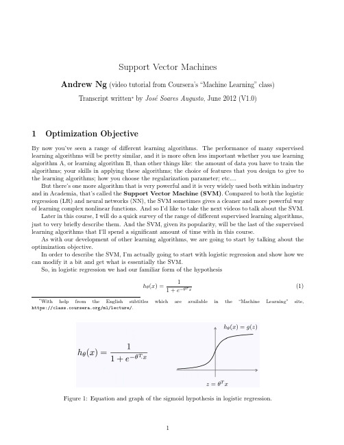
Support vector machine:A tool for mapping mineral prospectivityRenguang Zuo a,n,Emmanuel John M.Carranza ba State Key Laboratory of Geological Processes and Mineral Resources,China University of Geosciences,Wuhan430074;Beijing100083,Chinab Department of Earth Systems Analysis,Faculty of Geo-Information Science and Earth Observation(ITC),University of Twente,Enschede,The Netherlandsa r t i c l e i n f oArticle history:Received17May2010Received in revised form3September2010Accepted25September2010Keywords:Supervised learning algorithmsKernel functionsWeights-of-evidenceTurbidite-hosted AuMeguma Terraina b s t r a c tIn this contribution,we describe an application of support vector machine(SVM),a supervised learningalgorithm,to mineral prospectivity mapping.The free R package e1071is used to construct a SVM withsigmoid kernel function to map prospectivity for Au deposits in western Meguma Terrain of Nova Scotia(Canada).The SVM classification accuracies of‘deposit’are100%,and the SVM classification accuracies ofthe‘non-deposit’are greater than85%.The SVM classifications of mineral prospectivity have5–9%lowertotal errors,13–14%higher false-positive errors and25–30%lower false-negative errors compared tothose of the WofE prediction.The prospective target areas predicted by both SVM and WofE reflect,nonetheless,controls of Au deposit occurrence in the study area by NE–SW trending anticlines andcontact zones between Goldenville and Halifax Formations.The results of the study indicate theusefulness of SVM as a tool for predictive mapping of mineral prospectivity.&2010Elsevier Ltd.All rights reserved.1.IntroductionMapping of mineral prospectivity is crucial in mineral resourcesexploration and mining.It involves integration of information fromdiverse geoscience datasets including geological data(e.g.,geologicalmap),geochemical data(e.g.,stream sediment geochemical data),geophysical data(e.g.,magnetic data)and remote sensing data(e.g.,multispectral satellite data).These sorts of data can be visualized,processed and analyzed with the support of computer and GIStechniques.Geocomputational techniques for mapping mineral pro-spectivity include weights of evidence(WofE)(Bonham-Carter et al.,1989),fuzzy WofE(Cheng and Agterberg,1999),logistic regression(Agterberg and Bonham-Carter,1999),fuzzy logic(FL)(Ping et al.,1991),evidential belief functions(EBF)(An et al.,1992;Carranza andHale,2003;Carranza et al.,2005),neural networks(NN)(Singer andKouda,1996;Porwal et al.,2003,2004),a‘wildcat’method(Carranza,2008,2010;Carranza and Hale,2002)and a hybrid method(e.g.,Porwalet al.,2006;Zuo et al.,2009).These techniques have been developed toquantify indices of occurrence of mineral deposit occurrence byintegrating multiple evidence layers.Some geocomputational techni-ques can be performed using popular software packages,such asArcWofE(a free ArcView extension)(Kemp et al.,1999),ArcSDM9.3(afree ArcGIS9.3extension)(Sawatzky et al.,2009),MI-SDM2.50(aMapInfo extension)(Avantra Geosystems,2006),GeoDAS(developedbased on MapObjects,which is an Environmental Research InstituteDevelopment Kit)(Cheng,2000).Other geocomputational techniques(e.g.,FL and NN)can be performed by using R and Matlab.Geocomputational techniques for mineral prospectivity map-ping can be categorized generally into two types–knowledge-driven and data-driven–according to the type of inferencemechanism considered(Bonham-Carter1994;Pan and Harris2000;Carranza2008).Knowledge-driven techniques,such as thosethat apply FL and EBF,are based on expert knowledge andexperience about spatial associations between mineral prospec-tivity criteria and mineral deposits of the type sought.On the otherhand,data-driven techniques,such as WofE and NN,are based onthe quantification of spatial associations between mineral pro-spectivity criteria and known occurrences of mineral deposits ofthe type sought.Additional,the mixing of knowledge-driven anddata-driven methods also is used for mapping of mineral prospec-tivity(e.g.,Porwal et al.,2006;Zuo et al.,2009).Every geocomputa-tional technique has advantages and disadvantages,and one or theother may be more appropriate for a given geologic environmentand exploration scenario(Harris et al.,2001).For example,one ofthe advantages of WofE is its simplicity,and straightforwardinterpretation of the weights(Pan and Harris,2000),but thismodel ignores the effects of possible correlations amongst inputpredictor patterns,which generally leads to biased prospectivitymaps by assuming conditional independence(Porwal et al.,2010).Comparisons between WofE and NN,NN and LR,WofE,NN and LRfor mineral prospectivity mapping can be found in Singer andKouda(1999),Harris and Pan(1999)and Harris et al.(2003),respectively.Mapping of mineral prospectivity is a classification process,because its product(i.e.,index of mineral deposit occurrence)forevery location is classified as either prospective or non-prospectiveaccording to certain combinations of weighted mineral prospec-tivity criteria.There are two types of classification techniques.Contents lists available at ScienceDirectjournal homepage:/locate/cageoComputers&Geosciences0098-3004/$-see front matter&2010Elsevier Ltd.All rights reserved.doi:10.1016/j.cageo.2010.09.014n Corresponding author.E-mail addresses:zrguang@,zrguang1981@(R.Zuo).Computers&Geosciences](]]]])]]]–]]]One type is known as supervised classification,which classifies mineral prospectivity of every location based on a training set of locations of known deposits and non-deposits and a set of evidential data layers.The other type is known as unsupervised classification, which classifies mineral prospectivity of every location based solely on feature statistics of individual evidential data layers.A support vector machine(SVM)is a model of algorithms for supervised classification(Vapnik,1995).Certain types of SVMs have been developed and applied successfully to text categorization, handwriting recognition,gene-function prediction,remote sensing classification and other studies(e.g.,Joachims1998;Huang et al.,2002;Cristianini and Scholkopf,2002;Guo et al.,2005; Kavzoglu and Colkesen,2009).An SVM performs classification by constructing an n-dimensional hyperplane in feature space that optimally separates evidential data of a predictor variable into two categories.In the parlance of SVM literature,a predictor variable is called an attribute whereas a transformed attribute that is used to define the hyperplane is called a feature.The task of choosing the most suitable representation of the target variable(e.g.,mineral prospectivity)is known as feature selection.A set of features that describes one case(i.e.,a row of predictor values)is called a feature vector.The feature vectors near the hyperplane are the support feature vectors.The goal of SVM modeling is tofind the optimal hyperplane that separates clusters of feature vectors in such a way that feature vectors representing one category of the target variable (e.g.,prospective)are on one side of the plane and feature vectors representing the other category of the target variable(e.g.,non-prospective)are on the other size of the plane.A good separation is achieved by the hyperplane that has the largest distance to the neighboring data points of both categories,since in general the larger the margin the better the generalization error of the classifier.In this paper,SVM is demonstrated as an alternative tool for integrating multiple evidential variables to map mineral prospectivity.2.Support vector machine algorithmsSupport vector machines are supervised learning algorithms, which are considered as heuristic algorithms,based on statistical learning theory(Vapnik,1995).The classical task of a SVM is binary (two-class)classification.Suppose we have a training set composed of l feature vectors x i A R n,where i(¼1,2,y,n)is the number of feature vectors in training samples.The class in which each sample is identified to belong is labeled y i,which is equal to1for one class or is equal toÀ1for the other class(i.e.y i A{À1,1})(Huang et al., 2002).If the two classes are linearly separable,then there exists a family of linear separators,also called separating hyperplanes, which satisfy the following set of equations(KavzogluandFig.1.Support vectors and optimum hyperplane for the binary case of linearly separable data sets.Table1Experimental data.yer A Layer B Layer C Layer D Target yer A Layer B Layer C Layer D Target1111112100000 2111112200000 3111112300000 4111112401000 5111112510000 6111112600000 7111112711100 8111112800000 9111012900000 10111013000000 11101113111100 12111013200000 13111013300000 14111013400000 15011013510000 16101013600000 17011013700000 18010113811100 19010112900000 20101014010000R.Zuo,E.J.M.Carranza/Computers&Geosciences](]]]])]]]–]]]2Colkesen,2009)(Fig.1):wx iþb Zþ1for y i¼þ1wx iþb rÀ1for y i¼À1ð1Þwhich is equivalent toy iðwx iþbÞZ1,i¼1,2,...,nð2ÞThe separating hyperplane can then be formalized as a decision functionfðxÞ¼sgnðwxþbÞð3Þwhere,sgn is a sign function,which is defined as follows:sgnðxÞ¼1,if x400,if x¼0À1,if x o08><>:ð4ÞThe two parameters of the separating hyperplane decision func-tion,w and b,can be obtained by solving the following optimization function:Minimize tðwÞ¼12J w J2ð5Þsubject toy Iððwx iÞþbÞZ1,i¼1,...,lð6ÞThe solution to this optimization problem is the saddle point of the Lagrange functionLðw,b,aÞ¼1J w J2ÀX li¼1a iðy iððx i wÞþbÞÀ1Þð7Þ@ @b Lðw,b,aÞ¼0@@wLðw,b,aÞ¼0ð8Þwhere a i is a Lagrange multiplier.The Lagrange function is minimized with respect to w and b and is maximized with respect to a grange multipliers a i are determined by the following optimization function:MaximizeX li¼1a iÀ12X li,j¼1a i a j y i y jðx i x jÞð9Þsubject toa i Z0,i¼1,...,l,andX li¼1a i y i¼0ð10ÞThe separating rule,based on the optimal hyperplane,is the following decision function:fðxÞ¼sgnX li¼1y i a iðxx iÞþb!ð11ÞMore details about SVM algorithms can be found in Vapnik(1995) and Tax and Duin(1999).3.Experiments with kernel functionsFor spatial geocomputational analysis of mineral exploration targets,the decision function in Eq.(3)is a kernel function.The choice of a kernel function(K)and its parameters for an SVM are crucial for obtaining good results.The kernel function can be usedTable2Errors of SVM classification using linear kernel functions.l Number ofsupportvectors Testingerror(non-deposit)(%)Testingerror(deposit)(%)Total error(%)0.2580.00.00.0180.00.00.0 1080.00.00.0 10080.00.00.0 100080.00.00.0Table3Errors of SVM classification using polynomial kernel functions when d¼3and r¼0. l Number ofsupportvectorsTestingerror(non-deposit)(%)Testingerror(deposit)(%)Total error(%)0.25120.00.00.0160.00.00.01060.00.00.010060.00.00.0 100060.00.00.0Table4Errors of SVM classification using polynomial kernel functions when l¼0.25,r¼0.d Number ofsupportvectorsTestingerror(non-deposit)(%)Testingerror(deposit)(%)Total error(%)11110.00.0 5.010290.00.00.0100230.045.022.5 1000200.090.045.0Table5Errors of SVM classification using polynomial kernel functions when l¼0.25and d¼3.r Number ofsupportvectorsTestingerror(non-deposit)(%)Testingerror(deposit)(%)Total error(%)0120.00.00.01100.00.00.01080.00.00.010080.00.00.0 100080.00.00.0Table6Errors of SVM classification using radial kernel functions.l Number ofsupportvectorsTestingerror(non-deposit)(%)Testingerror(deposit)(%)Total error(%)0.25140.00.00.01130.00.00.010130.00.00.0100130.00.00.0 1000130.00.00.0Table7Errors of SVM classification using sigmoid kernel functions when r¼0.l Number ofsupportvectorsTestingerror(non-deposit)(%)Testingerror(deposit)(%)Total error(%)0.25400.00.00.01400.035.017.510400.0 6.0 3.0100400.0 6.0 3.0 1000400.0 6.0 3.0R.Zuo,E.J.M.Carranza/Computers&Geosciences](]]]])]]]–]]]3to construct a non-linear decision boundary and to avoid expensive calculation of dot products in high-dimensional feature space.The four popular kernel functions are as follows:Linear:Kðx i,x jÞ¼l x i x j Polynomial of degree d:Kðx i,x jÞ¼ðl x i x jþrÞd,l40Radial basis functionðRBFÞ:Kðx i,x jÞ¼exp fÀl99x iÀx j992g,l40 Sigmoid:Kðx i,x jÞ¼tanhðl x i x jþrÞ,l40ð12ÞThe parameters l,r and d are referred to as kernel parameters. The parameter l serves as an inner product coefficient in the polynomial function.In the case of the RBF kernel(Eq.(12)),l determines the RBF width.In the sigmoid kernel,l serves as an inner product coefficient in the hyperbolic tangent function.The parameter r is used for kernels of polynomial and sigmoid types. The parameter d is the degree of a polynomial function.We performed some experiments to explore the performance of the parameters used in a kernel function.The dataset used in the experiments(Table1),which are derived from the study area(see below),were compiled according to the requirementfor Fig.2.Simplified geological map in western Meguma Terrain of Nova Scotia,Canada(after,Chatterjee1983;Cheng,2008).Table8Errors of SVM classification using sigmoid kernel functions when l¼0.25.r Number ofSupportVectorsTestingerror(non-deposit)(%)Testingerror(deposit)(%)Total error(%)0400.00.00.01400.00.00.010400.00.00.0100400.00.00.01000400.00.00.0R.Zuo,E.J.M.Carranza/Computers&Geosciences](]]]])]]]–]]]4classification analysis.The e1071(Dimitriadou et al.,2010),a freeware R package,was used to construct a SVM.In e1071,the default values of l,r and d are1/(number of variables),0and3,respectively.From the study area,we used40geological feature vectors of four geoscience variables and a target variable for classification of mineral prospec-tivity(Table1).The target feature vector is either the‘non-deposit’class(or0)or the‘deposit’class(or1)representing whether mineral exploration target is absent or present,respectively.For‘deposit’locations,we used the20known Au deposits.For‘non-deposit’locations,we randomly selected them according to the following four criteria(Carranza et al.,2008):(i)non-deposit locations,in contrast to deposit locations,which tend to cluster and are thus non-random, must be random so that multivariate spatial data signatures are highly non-coherent;(ii)random non-deposit locations should be distal to any deposit location,because non-deposit locations proximal to deposit locations are likely to have similar multivariate spatial data signatures as the deposit locations and thus preclude achievement of desired results;(iii)distal and random non-deposit locations must have values for all the univariate geoscience spatial data;(iv)the number of distal and random non-deposit locations must be equaltoFig.3.Evidence layers used in mapping prospectivity for Au deposits(from Cheng,2008):(a)and(b)represent optimum proximity to anticline axes(2.5km)and contacts between Goldenville and Halifax formations(4km),respectively;(c)and(d)represent,respectively,background and anomaly maps obtained via S-Afiltering of thefirst principal component of As,Cu,Pb and Zn data.R.Zuo,E.J.M.Carranza/Computers&Geosciences](]]]])]]]–]]]5the number of deposit locations.We used point pattern analysis (Diggle,1983;2003;Boots and Getis,1988)to evaluate degrees of spatial randomness of sets of non-deposit locations and tofind distance from any deposit location and corresponding probability that one deposit location is situated next to another deposit location.In the study area,we found that the farthest distance between pairs of Au deposits is71km,indicating that within that distance from any deposit location in there is100%probability of another deposit location. However,few non-deposit locations can be selected beyond71km of the individual Au deposits in the study area.Instead,we selected random non-deposit locations beyond11km from any deposit location because within this distance from any deposit location there is90% probability of another deposit location.When using a linear kernel function and varying l from0.25to 1000,the number of support vectors and the testing errors for both ‘deposit’and‘non-deposit’do not vary(Table2).In this experiment the total error of classification is0.0%,indicating that the accuracy of classification is not sensitive to the choice of l.With a polynomial kernel function,we tested different values of l, d and r as follows.If d¼3,r¼0and l is increased from0.25to1000,the number of support vectors decreases from12to6,but the testing errors for‘deposit’and‘non-deposit’remain nil(Table3).If l¼0.25, r¼0and d is increased from1to1000,the number of support vectors firstly increases from11to29,then decreases from23to20,the testing error for‘non-deposit’decreases from10.0%to0.0%,whereas the testing error for‘deposit’increases from0.0%to90%(Table4). In this experiment,the total error of classification is minimum(0.0%) when d¼10(Table4).If l¼0.25,d¼3and r is increased from 0to1000,the number of support vectors decreases from12to8,but the testing errors for‘deposit’and‘non-deposit’remain nil(Table5).When using a radial kernel function and varying l from0.25to 1000,the number of support vectors decreases from14to13,but the testing errors of‘deposit’and‘non-deposit’remain nil(Table6).With a sigmoid kernel function,we experimented with different values of l and r as follows.If r¼0and l is increased from0.25to1000, the number of support vectors is40,the testing errors for‘non-deposit’do not change,but the testing error of‘deposit’increases from 0.0%to35.0%,then decreases to6.0%(Table7).In this experiment,the total error of classification is minimum at0.0%when l¼0.25 (Table7).If l¼0.25and r is increased from0to1000,the numbers of support vectors and the testing errors of‘deposit’and‘non-deposit’do not change and the total error remains nil(Table8).The results of the experiments demonstrate that,for the datasets in the study area,a linear kernel function,a polynomial kernel function with d¼3and r¼0,or l¼0.25,r¼0and d¼10,or l¼0.25and d¼3,a radial kernel function,and a sigmoid kernel function with r¼0and l¼0.25are optimal kernel functions.That is because the testing errors for‘deposit’and‘non-deposit’are0%in the SVM classifications(Tables2–8).Nevertheless,a sigmoid kernel with l¼0.25and r¼0,compared to all the other kernel functions,is the most optimal kernel function because it uses all the input support vectors for either‘deposit’or‘non-deposit’(Table1)and the training and testing errors for‘deposit’and‘non-deposit’are0% in the SVM classification(Tables7and8).4.Prospectivity mapping in the study areaThe study area is located in western Meguma Terrain of Nova Scotia,Canada.It measures about7780km2.The host rock of Au deposits in this area consists of Cambro-Ordovician low-middle grade metamorphosed sedimentary rocks and a suite of Devonian aluminous granitoid intrusions(Sangster,1990;Ryan and Ramsay, 1997).The metamorphosed sedimentary strata of the Meguma Group are the lower sand-dominatedflysch Goldenville Formation and the upper shalyflysch Halifax Formation occurring in the central part of the study area.The igneous rocks occur mostly in the northern part of the study area(Fig.2).In this area,20turbidite-hosted Au deposits and occurrences (Ryan and Ramsay,1997)are found in the Meguma Group, especially near the contact zones between Goldenville and Halifax Formations(Chatterjee,1983).The major Au mineralization-related geological features are the contact zones between Gold-enville and Halifax Formations,NE–SW trending anticline axes and NE–SW trending shear zones(Sangster,1990;Ryan and Ramsay, 1997).This dataset has been used to test many mineral prospec-tivity mapping algorithms(e.g.,Agterberg,1989;Cheng,2008). More details about the geological settings and datasets in this area can be found in Xu and Cheng(2001).We used four evidence layers(Fig.3)derived and used by Cheng (2008)for mapping prospectivity for Au deposits in the yers A and B represent optimum proximity to anticline axes(2.5km) and optimum proximity to contacts between Goldenville and Halifax Formations(4km),yers C and D represent variations in geochemical background and anomaly,respectively, as modeled by multifractalfilter mapping of thefirst principal component of As,Cu,Pb,and Zn data.Details of how the four evidence layers were obtained can be found in Cheng(2008).4.1.Training datasetThe application of SVM requires two subsets of training loca-tions:one training subset of‘deposit’locations representing presence of mineral deposits,and a training subset of‘non-deposit’locations representing absence of mineral deposits.The value of y i is1for‘deposits’andÀ1for‘non-deposits’.For‘deposit’locations, we used the20known Au deposits(the sixth column of Table1).For ‘non-deposit’locations(last column of Table1),we obtained two ‘non-deposit’datasets(Tables9and10)according to the above-described selection criteria(Carranza et al.,2008).We combined the‘deposits’dataset with each of the two‘non-deposit’datasets to obtain two training datasets.Each training dataset commonly contains20known Au deposits but contains different20randomly selected non-deposits(Fig.4).4.2.Application of SVMBy using the software e1071,separate SVMs both with sigmoid kernel with l¼0.25and r¼0were constructed using the twoTable9The value of each evidence layer occurring in‘non-deposit’dataset1.yer A Layer B Layer C Layer D100002000031110400005000061000700008000090100 100100 110000 120000 130000 140000 150000 160100 170000 180000 190100 200000R.Zuo,E.J.M.Carranza/Computers&Geosciences](]]]])]]]–]]] 6training datasets.With training dataset1,the classification accuracies for‘non-deposits’and‘deposits’are95%and100%, respectively;With training dataset2,the classification accuracies for‘non-deposits’and‘deposits’are85%and100%,respectively.The total classification accuracies using the two training datasets are97.5%and92.5%,respectively.The patterns of the predicted prospective target areas for Au deposits(Fig.5)are defined mainly by proximity to NE–SW trending anticlines and proximity to contact zones between Goldenville and Halifax Formations.This indicates that‘geology’is better than‘geochemistry’as evidence of prospectivity for Au deposits in this area.With training dataset1,the predicted prospective target areas occupy32.6%of the study area and contain100%of the known Au deposits(Fig.5a).With training dataset2,the predicted prospec-tive target areas occupy33.3%of the study area and contain95.0% of the known Au deposits(Fig.5b).In contrast,using the same datasets,the prospective target areas predicted via WofE occupy 19.3%of study area and contain70.0%of the known Au deposits (Cheng,2008).The error matrices for two SVM classifications show that the type1(false-positive)and type2(false-negative)errors based on training dataset1(Table11)and training dataset2(Table12)are 32.6%and0%,and33.3%and5%,respectively.The total errors for two SVM classifications are16.3%and19.15%based on training datasets1and2,respectively.In contrast,the type1and type2 errors for the WofE prediction are19.3%and30%(Table13), respectively,and the total error for the WofE prediction is24.65%.The results show that the total errors of the SVM classifications are5–9%lower than the total error of the WofE prediction.The 13–14%higher false-positive errors of the SVM classifications compared to that of the WofE prediction suggest that theSVMFig.4.The locations of‘deposit’and‘non-deposit’.Table10The value of each evidence layer occurring in‘non-deposit’dataset2.yer A Layer B Layer C Layer D110102000030000411105000060110710108000091000101110111000120010131000140000150000161000171000180010190010200000R.Zuo,E.J.M.Carranza/Computers&Geosciences](]]]])]]]–]]]7classifications result in larger prospective areas that may not contain undiscovered deposits.However,the 25–30%higher false-negative error of the WofE prediction compared to those of the SVM classifications suggest that the WofE analysis results in larger non-prospective areas that may contain undiscovered deposits.Certainly,in mineral exploration the intentions are notto miss undiscovered deposits (i.e.,avoid false-negative error)and to minimize exploration cost in areas that may not really contain undiscovered deposits (i.e.,keep false-positive error as low as possible).Thus,results suggest the superiority of the SVM classi-fications over the WofE prediction.5.ConclusionsNowadays,SVMs have become a popular geocomputational tool for spatial analysis.In this paper,we used an SVM algorithm to integrate multiple variables for mineral prospectivity mapping.The results obtained by two SVM applications demonstrate that prospective target areas for Au deposits are defined mainly by proximity to NE–SW trending anticlines and to contact zones between the Goldenville and Halifax Formations.In the study area,the SVM classifications of mineral prospectivity have 5–9%lower total errors,13–14%higher false-positive errors and 25–30%lower false-negative errors compared to those of the WofE prediction.These results indicate that SVM is a potentially useful tool for integrating multiple evidence layers in mineral prospectivity mapping.Table 11Error matrix for SVM classification using training dataset 1.Known All ‘deposits’All ‘non-deposits’TotalPrediction ‘Deposit’10032.6132.6‘Non-deposit’067.467.4Total100100200Type 1(false-positive)error ¼32.6.Type 2(false-negative)error ¼0.Total error ¼16.3.Note :Values in the matrix are percentages of ‘deposit’and ‘non-deposit’locations.Table 12Error matrix for SVM classification using training dataset 2.Known All ‘deposits’All ‘non-deposits’TotalPrediction ‘Deposits’9533.3128.3‘Non-deposits’566.771.4Total100100200Type 1(false-positive)error ¼33.3.Type 2(false-negative)error ¼5.Total error ¼19.15.Note :Values in the matrix are percentages of ‘deposit’and ‘non-deposit’locations.Table 13Error matrix for WofE prediction.Known All ‘deposits’All ‘non-deposits’TotalPrediction ‘Deposit’7019.389.3‘Non-deposit’3080.7110.7Total100100200Type 1(false-positive)error ¼19.3.Type 2(false-negative)error ¼30.Total error ¼24.65.Note :Values in the matrix are percentages of ‘deposit’and ‘non-deposit’locations.Fig.5.Prospective targets area for Au deposits delineated by SVM.(a)and (b)are obtained using training dataset 1and 2,respectively.R.Zuo,E.J.M.Carranza /Computers &Geosciences ](]]]])]]]–]]]8。

人工智能课程项目报告姓名： ******班级：**************目录一、实验背景 (1)二、实验目的 (1)三、实验原理 (1)3.1线性可分： (1)3.2线性不可分： (4)3.3坐标上升法： (7)3.4 SMO算法： (8)四、实验内容 (10)五、实验结果与分析 (12)5.1 实验环境与工具 (12)5.2 实验数据集与参数设置 (12)5.3 评估标准 (13)5.4 实验结果与分析 (13)一、实验背景本学期学习了高级人工智能课程，对人工智能的各方面知识有了新的认识和了解。

为了更好的深入学习人工智能的相关知识，决定以数据挖掘与机器学习的基础算法为研究对象，进行算法的研究与实现。

在数据挖掘的各种算法中，有一种分类算法的分类效果，在大多数情况下都非常的好，它就是支持向量机（SVM）算法。

这种算法的理论基础强，有着严格的推导论证，是研究和学习数据挖掘算法的很好的切入点。

二、实验目的对SVM算法进行研究与实现，掌握理论推导过程，培养严谨治学的科研态度。

三、实验原理支持向量机基本上是最好的有监督学习算法。

SVM由Vapnik首先提出(Boser,Guyon and Vapnik,1992;Cortes and Vapnik,1995;Vapnik, 1995,1998)。

它的主要思想是建立一个超平面作为决策曲面,使得正例和反例之间的隔离边缘被最大化。

SVM的优点:1.通用性(能够在各种函数集中构造函数)2.鲁棒性(不需要微调)3.有效性(在解决实际问题中属于最好的方法之一)4.计算简单(方法的实现只需要利用简单的优化技术)5.理论上完善(基于VC推广理论的框架)3.1线性可分：首先讨论线性可分的情况，线性不可分可以通过数学的手段变成近似线性可分。

基本模型：这里的裕量是几何间隔。

我们的目标是最大化几何间隔，但是看过一些关于SVM的论文的人一定记得什么优化的目标是要最小化||w||这样的说法，这是怎么回事呢？原因来自于对间隔和几何间隔的定义（数学基础）：间隔：δ=y(wx+b)=|g(x)|几何间隔：||w||叫做向量w的范数，范数是对向量长度的一种度量。

机器学习实际应用中必须考虑到的9个问题张皓AI科技大本营如今，机器学习变得十分诱人，它已在网页搜索、商品推荐、垃圾邮件检测、语音识别、图像识别以及自然语言处理等诸多领域发挥重要作用。

和以往我们显式地通过编程告诉计算机如何进行计算不同，机器学习是一种数据驱动方法(data-driven approach)。

然而，有时候机器学习像是一种'魔术'，即使是给定相同的数据，一位机器学习领域专家和一位新手训练得到的结果可能相去甚远。

本文简要讨论了实际应用机器学习时九个需要注意的重要方面。

作者| 张皓整理| AI科技大本营（微信ID：rgznai100）我该选什么学习算法?这可能是你面对一个具体应用场景想到的第一个问题。

你可能会想'机器学习里面这么多算法，究竟哪个算法最好'。

很'不幸'的是，没有免费午餐定理(No Free LunchTheorem)告诉我们对于任意两个学习算法，如果其中一个在某些问题上比另一个好，那么一定存在一些问题另一个学习算法（表现会）更好。

因此如果考虑所有可能问题，所有算法都一样好。

'好吧'，你可能会接着想，'没有免费午餐定理假定所有问题都有相同机会发生，但我只关心对我现在面对的问题，哪个算法更好'。

又很'不幸'的是，有可能你把机器学习里面所谓'十大算法'都试了一遍，然后感觉机器学习'这东西根本没用，这些算法我都试了，没一个效果好的'。

前一段时间'约战比武'的话题很热，其实机器学习和练武术有点像，把太极二十四式朝对方打一遍结果对方应声倒下这是不可能的。

机器学习算法是有限的，而现实应用问题是无限的，以有限的套路应对无限的变化，一定是会存在有的问题你无法用现有的算法解决的，岂有不败之理？因此，该选什么学习算法要和你要解决的具体问题相结合。

不同的学习算法有不同的归纳偏好(inductive bias)，你使用的算法的归纳偏好是否适应要解决的具体问题直接决定了学得模型的性能，有时你可能需要改造现有算法以应对你要解决的现实问题。

支持向量机的matlab代码Matlab中关于evalin帮助：EVALIN(WS,'expression') evaluates 'expression' in the context of the workspace WS. WS can be 'caller' or 'base'. It is similar to EVAL except that you can control which workspace the expression is evaluated in.[X,Y,Z,...] = EVALIN(WS,'expression') returns output arguments from the expression.EVALIN(WS,'try','catch') tries to evaluate the 'try' expression and if that fails it evaluates the 'catch' expression (in the current workspace).可知evalin('base', 'algo')是对工作空间base中的algo求值（返回其值）。

如果是7.0以上版本>>edit svmtrain>>edit svmclassify>>edit svmpredictfunction [svm_struct, svIndex] = svmtrain(training, groupnames, varargin)%SVMTRAIN trains a support vector machine classifier%% SVMStruct = SVMTRAIN(TRAINING,GROUP) trains a support vector machine % classifier using data TRAINING taken from two groups given by GROUP.% SVMStruct contains information about the trained classifier that is% used by SVMCLASSIFY for classification. GROUP is a column vector of% values of the same length as TRAINING that defines two groups. Each% element of GROUP specifies the group the corresponding row of TRAINING % belongs to. GROUP can be a numeric vector, a string array, or a cell% array of strings. SVMTRAIN treats NaNs or empty strings in GROUP as% missing values and ignores the corresponding rows of TRAINING.%% SVMTRAIN(...,'KERNEL_FUNCTION',KFUN) allows you to specify the kernel % function KFUN used to map the training data into kernel space. The% default kernel function is the dot product. KFUN can be one of the% following strings or a function handle:%% 'linear' Linear kernel or dot product% 'quadratic' Quadratic kernel% 'polynomial' Polynomial kernel (default order 3)% 'rbf' Gaussian Radial Basis Function kernel% 'mlp' Multilayer Perceptron kernel (default scale 1)% function A kernel function specified using @,% for example @KFUN, or an anonymous function%% A kernel function must be of the form%% function K = KFUN(U, V)%% The returned value, K, is a matrix of size M-by-N, where U and V have M% and N rows respectively. If KFUN is parameterized, you can use% anonymous functions to capture the problem-dependent parameters. For % example, suppose that your kernel function is%% function k = kfun(u,v,p1,p2)% k = tanh(p1*(u*v')+p2);%% You can set values for p1 and p2 and then use an anonymous function:% @(u,v) kfun(u,v,p1,p2).%% SVMTRAIN(...,'POLYORDER',ORDER) allows you to specify the order of a% polynomial kernel. The default order is 3.%% SVMTRAIN(...,'MLP_PARAMS',[P1 P2]) allows you to specify the% parameters of the Multilayer Perceptron (mlp) kernel. The mlp kernel% requires two parameters, P1 and P2, where K = tanh(P1*U*V' + P2) and P1 % > 0 and P2 < 0. Default values are P1 = 1 and P2 = -1.%% SVMTRAIN(...,'METHOD',METHOD) allows you to specify the method used % to find the separating hyperplane. Options are%% 'QP' Use quadratic programming (requires the Optimization Toolbox)% 'LS' Use least-squares method%% If you have the Optimization Toolbox, then the QP method is the default% method. If not, the only available method is LS.%% SVMTRAIN(...,'QUADPROG_OPTS',OPTIONS) allows you to pass an OPTIONS % structure created using OPTIMSET to the QUADPROG function when using % the 'QP' method. See help optimset for more details.%% SVMTRAIN(...,'SHOWPLOT',true), when used with two-dimensional data,% creates a plot of the grouped data and plots the separating line for% the classifier.%% Example:% % Load the data and select features for classification% load fisheriris% data = [meas(:,1), meas(:,2)];% % Extract the Setosa class% groups = ismember(species,'setosa');% % Randomly select training and test sets% [train, test] = crossvalind('holdOut',groups);% cp = classperf(groups);% % Use a linear support vector machine classifier% svmStruct = svmtrain(data(train,:),groups(train),'showplot',true); % classes = svmclassify(svmStruct,data(test,:),'showplot',true);% % See how well the classifier performed% classperf(cp,classes,test);% cp.CorrectRate%% See also CLASSIFY, KNNCLASSIFY, QUADPROG, SVMCLASSIFY.% Copyright 2004 The MathWorks, Inc.% $Revision: 1.1.12.1 $ $Date: 2004/12/24 20:43:35 $% References:% [1] Kecman, V, Learning and Soft Computing,% MIT Press, Cambridge, MA. 2001.% [2] Suykens, J.A.K., Van Gestel, T., De Brabanter, J., De Moor, B., % Vandewalle, J., Least Squares Support Vector Machines,% World Scientific, Singapore, 2002.% [3] Scholkopf, B., Smola, A.J., Learning with Kernels,% MIT Press, Cambridge, MA. 2002.%% SVMTRAIN(...,'KFUNARGS',ARGS) allows you to pass additional% arguments to kernel functions.% set defaultsplotflag = false;qp_opts = [];kfunargs = {};setPoly = false; usePoly = false;setMLP = false; useMLP = false;if ~isempty(which('quadprog'))useQuadprog = true;elseuseQuadprog = false;% set default kernel functionkfun = @linear_kernel;% check inputsif nargin < 2error(nargchk(2,Inf,nargin))endnumoptargs = nargin -2;optargs = varargin;% grp2idx sorts a numeric grouping var ascending, and a string grouping % var by order of first occurrence[g,groupString] = grp2idx(groupnames);% check group is a vector -- though char input is special...if ~isvector(groupnames) && ~ischar(groupnames)error('Bioinfo:svmtrain:GroupNotVector',...'Group must be a vector.');end% make sure that the data is correctly oriented.if size(groupnames,1) == 1groupnames = groupnames';end% make sure data is the right sizen = length(groupnames);if size(training,1) ~= nif size(training,2) == ntraining = training';elseerror('Bioinfo:svmtrain:DataGroupSizeMismatch',...'GROUP and TRAINING must have the same number of rows.')endend% NaNs are treated as unknown classes and are removed from the training % datanans = find(isnan(g));if length(nans) > 0training(nans,:) = [];g(nans) = [];ngroups = length(groupString);if ngroups > 2error('Bioinfo:svmtrain:TooManyGroups',...'SVMTRAIN only supports classification into two groups.\nGROUP contains %d different groups.',ngroups)end% convert to 1, -1.g = 1 - (2* (g-1));% handle optional argumentsif numoptargs >= 1if rem(numoptargs,2)== 1error('Bioinfo:svmtrain:IncorrectNumberOfArguments',...'Incorrect number of arguments to %s.',mfilename);endokargs = {'kernel_function','method','showplot','kfunargs','quadprog_opts','polyorder',' mlp_params'};for j=1:2:numoptargspname = optargs{j};pval = optargs{j+1};k = strmatch(lower(pname), okargs);%#okif isempty(k)error('Bioinfo:svmtrain:UnknownParameterName',...'Unknown parameter name: %s.',pname);elseif length(k)>1error('Bioinfo:svmtrain:AmbiguousParameterName',...'Ambiguous parameter name: %s.',pname);elseswitch(k)case 1 % kernel_functionif ischar(pval)okfuns = {'linear','quadratic',...'radial','rbf','polynomial','mlp'};funNum = strmatch(lower(pval), okfuns);%#okif isempty(funNum)funNum = 0;endswitch funNum %maybe make this less strict in the futurecase 1kfun = @linear_kernel;kfun = @quadratic_kernel;case {3,4}kfun = @rbf_kernel;case 5kfun = @poly_kernel;usePoly = true;case 6kfun = @mlp_kernel;useMLP = true;otherwiseerror('Bioinfo:svmtrain:UnknownKernelFunction',...'Unknown Kernel Function %s.',kfun);endelseif isa (pval, 'function_handle')kfun = pval;elseerror('Bioinfo:svmtrain:BadKernelFunction',...'The kernel function input does not appear to be a function handle\nor valid function name.')endcase 2 % methodif strncmpi(pval,'qp',2)useQuadprog = true;if isempty(which('quadprog'))warning('Bioinfo:svmtrain:NoOptim',...'The Optimization Toolbox is required to use the quadratic programming method.')useQuadprog = false;endelseif strncmpi(pval,'ls',2)useQuadprog = false;elseerror('Bioinfo:svmtrain:UnknownMethod',...'Unknown method option %s. Valid methods are ''QP'' and ''LS''',pval);endcase 3 % displayif pval ~= 0if size(training,2) == 2plotflag = true;elsewarning('Bioinfo:svmtrain:OnlyPlot2D',...'The display option can only plot 2D training data.')endcase 4 % kfunargsif iscell(pval)kfunargs = pval;elsekfunargs = {pval};endcase 5 % quadprog_optsif isstruct(pval)qp_opts = pval;elseif iscell(pval)qp_opts = optimset(pval{:});elseerror('Bioinfo:svmtrain:BadQuadprogOpts',...'QUADPROG_OPTS must be an opts structure.');endcase 6 % polyorderif ~isscalar(pval) || ~isnumeric(pval)error('Bioinfo:svmtrain:BadPolyOrder',...'POLYORDER must be a scalar value.');endif pval ~=floor(pval) || pval < 1error('Bioinfo:svmtrain:PolyOrderNotInt',...'The order of the polynomial kernel must be a positive integer.')endkfunargs = {pval};setPoly = true;case 7 % mlpparamsif numel(pval)~=2error('Bioinfo:svmtrain:BadMLPParams',...'MLP_PARAMS must be a two element array.');endif ~isscalar(pval(1)) || ~isscalar(pval(2))error('Bioinfo:svmtrain:MLPParamsNotScalar',...'The parameters of the multi-layer perceptron kernel must be scalar.'); endkfunargs = {pval(1),pval(2)};setMLP = true;endendendif setPoly && ~usePolywarning('Bioinfo:svmtrain:PolyOrderNotPolyKernel',...'You specified a polynomial order but not a polynomial kernel');endif setMLP && ~useMLPwarning('Bioinfo:svmtrain:MLPParamNotMLPKernel',...'You specified MLP parameters but not an MLP kernel');end% plot the data if requestedif plotflag[hAxis,hLines] = svmplotdata(training,g);legend(hLines,cellstr(groupString));end% calculate kernel functiontrykx = feval(kfun,training,training,kfunargs{:});% ensure function is symmetrickx = (kx+kx')/2;catcherror('Bioinfo:svmtrain:UnknownKernelFunction',...'Error calculating the kernel function:\n%s\n', lasterr);end% create Hessian% add small constant eye to force stabilityH =((g*g').*kx) + sqrt(eps(class(training)))*eye(n);if useQuadprog% The large scale solver cannot handle this type of problem, so turn it % off.qp_opts = optimset(qp_opts,'LargeScale','Off');% X=QUADPROG(H,f,A,b,Aeq,beq,LB,UB,X0,opts)alpha = quadprog(H,-ones(n,1),[],[],...g',0,zeros(n,1),inf *ones(n,1),zeros(n,1),qp_opts);% The support vectors are the non-zeros of alphasvIndex = find(alpha > sqrt(eps));sv = training(svIndex,:);% calculate the parameters of the separating line from the support% vectors.alphaHat = g(svIndex).*alpha(svIndex);% Calculate the bias by applying the indicator function to the support% vector with largest alpha.[maxAlpha,maxPos] = max(alpha); %#okbias = g(maxPos) - sum(alphaHat.*kx(svIndex,maxPos));% an alternative method is to average the values over all support vectors% bias = mean(g(sv)' - sum(alphaHat(:,ones(1,numSVs)).*kx(sv,sv)));% An alternative way to calculate support vectors is to look for zeros of% the Lagrangians (fifth output from QUADPROG).%% [alpha,fval,output,exitflag,t] = quadprog(H,-ones(n,1),[],[],...% g',0,zeros(n,1),inf *ones(n,1),zeros(n,1),opts);%% sv = t.lower < sqrt(eps) & t.upper < sqrt(eps);else % Least-Squares% now build up compound matrix for solverA = [0 g';g,H];b = [0;ones(size(g))];x = A\b;% calculate the parameters of the separating line from the support% vectors.sv = training;bias = x(1);alphaHat = g.*x(2:end);endsvm_struct.SupportVectors = sv;svm_struct.Alpha = alphaHat;svm_struct.Bias = bias;svm_struct.KernelFunction = kfun;svm_struct.KernelFunctionArgs = kfunargs;svm_struct.GroupNames = groupnames;svm_struct.FigureHandles = [];if plotflaghSV = svmplotsvs(hAxis,svm_struct);svm_struct.FigureHandles = {hAxis,hLines,hSV};endsvm的通俗理解3.5.1 线性可分条件下的支持向量机最优分界面Vapnik等人在多年研究统计学习理论基础上对线性分类器提出了另一种设计最佳准则。