博弈论讲义2

Last Time:Defined knowledge, common knowledge, meet (of partitions), and reachability.Reminders:• E is common knowledge at ω if ()I K E ω∞∈.• “Reachability Lemma” :'()M ωω∈ if there is a chain of states 01,,...m 'ωωωωω== such that for each k ω there is a player i(k) s.t. ()()1()(i k k i k k h h )ωω+=:• Theorem: Event E is common knowledge at ωiff ()M E ω⊆.How does set of NE change with information structure?Suppose there is a finite number of payoff matrices 1,...,L u u for finite strategy sets 1,...,I S SState space Ω, common prior p, partitions , and a map i H λso that payoff functions in state ω are ()(.)u λω; the strategy spaces are maps from into . i H i SWhen the state space is finite, this is a finite game, and we know that NE is u.h.c. and generically l.h.c. in p. In particular, it will be l.h.c. at strict NE.The “coordinated attack” game8,810,11,100,0A B A B-- 0,010,11,108,8A B A B--a ub uΩ= 0,1,2,….In state 0: payoff functions are given by matrix ; bu In all other states payoff functions are given by . a upartitions of Ω1H : (0), (1,2), (3,4),… (2n-1,2n)... 2H (0,1),(2,3). ..(2n,2n+1)…Prior p : p(0)=2/3, p(k)= for k>0 and 1(1)/3k e e --(0,1)ε∈.Interpretation: coordinated attack/email:Player 1 observes Nature’s choice of payoff matrix, sends a message to player 2.Sending messages isn’t a strategic decision, it’s hard-coded.Suppose state is n=2k >0. Then 1 knows the payoffs, knows 2 knows them. Moreover 2 knows that 1knows that 2 knows, and so on up to strings of length k: . 1(0n I n K n -Î>)But there is no state at which n>0 is c.k. (to see this, use reachability…).When it is c.k. that payoff are given by , (A,A) is a NE. But.. auClaim: the only NE is “play B at every information set.”.Proof: player 1 plays B in state 0 (payoff matrix ) since it strictly dominates A. b uLet , and note that .(0|(0,1))q p =1/2q >Now consider player 2 at information set (0,1).Since player 1 plays B in state 0, and the lowest payoff 2 can get to B in state 1 is 0, player 2’s expected payoff to B at (0,1) is at least 8. qPlaying A gives at most 108(1)q q −+−, and since , playing B is better. 1/2q >Now look at player 1 at 1(1,2)h =. Let q'=p(1|1,2), and note that '1(1)q /2εεεε=>+−.Since 2 plays B in state 1, player 1's payoff to B is at least 8q';1’s payoff to A is at most -10q'+8(1-q) so 1 plays B Now iterate..Conclude that the unique NE is always B- there is no NE in which at some state the outcome is (A,A).But (A,A ) is a strict NE of the payoff matrix . a u And at large n, there is mutual knowledge of the payoffs to high order- 1 knows that 2 knows that …. n/2 times. So “mutual knowledge to large n” has different NE than c.k.Also, consider "expanded games" with state space . 0,1,....,...n Ω=∞For each small positive ε let the distribution p ε be as above: 1(0)2/3,()(1)/3n p p n ee e e -==- for 0 and n <<∞()0p ε∞=.Define distribution by *p *(0)2/3p =,. *()1/3p ∞=As 0ε→, probability mass moves to higher n, andthere is a sense in which is the limit of the *p p εas 0ε→.But if we do say that *p p ε→ we have a failure of lower hemi continuity at a strict NE.So maybe we don’t want to say *p p ε→, and we don’t want to use mutual knowledge to large n as a notion of almost common knowledge.So the questions:• When should we say that one information structure is close to another?• What should we mean by "almost common knowledge"?This last question is related because we would like to say that an information structure where a set of events E is common knowledge is close to another information structure where these events are almost common knowledge.Monderer-Samet: Player i r-believes E at ω if (|())i p E h r ω≥.()r i B E is the set of all ω where player i r- believesE; this is also denoted 1.()ri B ENow do an iterative definition in the style of c.k.: 11()()rr I i i B E B E =Ç (everyone r-believes E) 1(){|(()|())}n r n ri i I B E p B E h r w w -=³ ()()n r n rI i i B E B =ÇEE is common r belief at ω if ()rI B E w ¥ÎAs with c.k., common r-belief can be characterized in terms of public events:• An event is a common r-truism if everyone r -believes it when it occurs.• An event is common r -belief at ω if it is implied by a common r-truism at ω.Now we have one version of "almost ck" : An event is almost ck if it is common r-belief for r near 1.MS show that if two player’s posteriors are common r-belief, they differ by at most 2(1-r): so Aumann's result is robust to almost ck, and holds in the limit.MS also that a strict NE of a game with knownpayoffs is still a NE when payoffs are "almost ck” - a form of lower hemi continuity.More formally:As before consider a family of games with fixed finite action spaces i A for each player i. a set of payoff matrices ,:l I u A R ->a state space W , that is now either finite or countably infinite, a prior p, a map such that :1,,,L l W®payoffs at ω are . ()(,)()w u a u a l w =Payoffs are common r-belief at ω if the event {|()}w l w l = is common r belief at ω.For each λ let λσ be a NE for common- knowledgepayoffs u .lDefine s * by *(())s l w w s =.This assigns each w a NE for the corresponding payoffs.In the email game, one such *s is . **(0)(,),()(,)s B B s n A A n ==0∀>If payoffs are c.k. at each ω, then s* is a NE of overall game G. (discuss)Theorem: Monder-Samet 1989Suppose that for each l , l s is a strict equilibrium for payoffs u λ.Then for any there is 0e >1r < and 1q < such that for all [,1]r r Î and [,1]q q Î,if there is probability q that payoffs are common r- belief, then there is a NE s of G with *(|()())1p s s ωωω=>ε−.Note that the conclusion of the theorem is false in the email game:there is no NE with an appreciable probability of playing A, even though (A,A) is a strict NE of the payoffs in every state but state 0.This is an indirect way of showing that the payoffs are never ACK in the email game.Now many payoff matrices don’t have strictequilibria, and this theorem doesn’t tell us anything about them.But can extend it to show that if for each state ω, *(s )ω is a Nash (but not necessarily strict Nash) equilibrium, then for any there is 0e >1r < and 1q < such that for all [,1]r r Î and [,1]q q Î, if payoffs are common r-belief with probability q, there is an “interim ε equilibria” of G where s * is played with probability 1ε−.Interim ε-equilibria:At each information set, the actions played are within epsilon of maxing expected payoff(((),())|())((',())|())i i i i i i i i E u s s h w E u s s h w w w w e-->=-Note that this implies the earlier result when *s specifies strict equilibria.Outline of proof:At states where some payoff function is common r-belief, specify that players follow s *. The key is that at these states, each player i r-believes that all other players r-believe the payoffs are common r-belief, so each expects the others to play according to s *.*ΩRegardless of play in the other states, playing this way is a best response, where k is a constant that depends on the set of possible payoff functions.4(1)k −rTo define play at states in */ΩΩconsider an artificial game where players are constrained to play s * in - and pick a NE of this game.*ΩThe overall strategy profile is an interim ε-equilibrium that plays like *s with probability q.To see the role of the infinite state space, consider the"truncated email game"player 2 does not respond after receiving n messages, so there are only 2n states.When 2n occurs: 2 knows it occurs.That is, . {}2(0,1),...(22,21,)(2)H n n =−−n n {}1(0),(1,2),...(21,2)H n =−.()2|(21,2)1p n n n ε−=−, so 2n is a "1-ε truism," and thus it is common 1-ε belief when it occurs.So there is an exact equilibrium where players playA in state 2n.More generally: on a finite state space, if the probability of an event is close to 1, then there is high probability that it is common r belief for r near 1.Not true on infinite state spaces…Lipman, “Finite order implications of the common prior assumption.”His point: there basically aren’t any!All of the "bite" of the CPA is in the tails.Set up: parameter Q that people "care about" States s S ∈,:f S →Θ specifies what the payoffs are at state s. Partitions of S, priors .i H i pPlayer i’s first order beliefs at s: the conditional distribution on Q given s.For B ⊆Θ,1()()i s B d =('|(')|())i i p s f s B h s ÎPlayer i’s second order beliefs: beliefs about Q and other players’ first order beliefs.()21()(){'|(('),('))}|()i i j i s B p s f s s B h d d =Îs and so on.The main point can be seen in his exampleTwo possible values of an unknown parameter r .1q q = o 2qStart with a model w/o common prior, relate it to a model with common prior.Starting model has only two states 12{,}S s s =. Each player has the trivial partition- ie no info beyond the prior.1122()()2/3p s p s ==.example: Player 1 owns an asset whose value is 1 at 1θ and 2 at 2θ; ()i i f s θ=.At each state, 1's expected value of the asset 4/3, 2's is 5/3, so it’s common knowledge that there are gains from trade.Lipman shows we can match the players’ beliefs, beliefs about beliefs, etc. to arbitrarily high order in a common prior model.Fix an integer N. construct the Nth model as followsState space'S ={1,...2}N S ´Common prior is that all states equally likely.The value of θ at (s,k) is determined by the s- component.Now we specify the partitions of each player in such a way that the beliefs, beliefs about beliefs, look like the simple model w/o common prior.1's partition: events112{(,1),(,2),(,1)}...s s s 112{(,21),(,2),(,)}s k s k s k -for k up to ; the “left-over” 12N -2s states go into 122{(,21),...(,2)}N N s s -+.At every event but the last one, 1 thinks the probability of is 2/3.1qThe partition for player 2 is similar but reversed: 221{(,21),(,2),(,)}s k s k s k - for k up to . 12N -And at all info sets but one, player 2 thinks the prob. of is 1/3.1qNow we look at beliefs at the state 1(,1)s .We matched the first-order beliefs (beliefs about θ) by construction)Now look at player 1's second-order beliefs.1 thinks there are 3 possible states 1(,1)s , 1(,2)s , 2(,1)s .At 1(,1)s , player 2 knows {1(,1)s ,2(,1)s ,(,}. 22)s At 1(,2)s , 2 knows . 122{(,2),(,3),(,4)}s s s At 2(,1)s , 2 knows {1(,2)s , 2(,1)s ,(,}. 22)sThe support of 1's second-order beliefs at 1(,1)s is the set of 2's beliefs at these info sets.And at each of them 2's beliefs are (1/3 1θ, 2/3 2θ). Same argument works up to N:The point is that the N-state models are "like" the original one in that beliefs at some states are the same as beliefs in the original model to high but finite order.(Beliefs at other states are very different- namely atθ or 2 is sure the states where 1 is sure that state is2θ.)it’s1Conclusion: if we assume that beliefs at a given state are generated by updating from a common prior, this doesn’t pin down their finite order behavior. So the main force of the CPA is on the entire infinite hierarchy of beliefs.Lipman goes on from this to make a point that is correct but potentially misleading: he says that "almost all" priors are close to a common. I think its misleading because here he uses the product topology on the set of hierarchies of beliefs- a.k.a topology of pointwise convergence.And two types that are close in this product topology can have very different behavior in a NE- so in a sense NE is not continuous in this topology.The email game is a counterexample. “Product Belief Convergence”:A sequence of types converges to if thesequence converges pointwise. That is, if for each k,, in t *i t ,,i i k n k *δδ→.Now consider the expanded version of the email game, where we added the state ∞.Let be the hierarchy of beliefs of player 1 when he has sent n messages, and let be the hierarchy atthe point ∞, where it is common knowledge that the payoff matrix is .in t ,*i t a uClaim: the sequence converges pointwise to . in t ,*i t Proof: At , i’s zero-order beliefs assignprobability 1 to , his first-order beliefs assignprobability 1 to ( and j knows it is ) and so onup to level n-1. Hence as n goes to infinity, thehierarchy of beliefs converges pointwise to common knowledge of .in t a u a u a u a uIn other words, if the number of levels of mutual knowledge go to infinity, then beliefs converge to common knowledge in the product topology. But we know that mutual knowledge to high order is not the same as almost common knowledge, and types that are close in the product topology can play very differently in Nash equilibrium.Put differently, the product topology on countably infinite sequences is insensitive to the tail of the sequence, but we know that the tail of the belief hierarchy can matter.Next : B-D JET 93 "Hierarchies of belief and Common Knowledge”.Here the hierarchies of belief are motivated by Harsanyi's idea of modelling incomplete information as imperfect information.Harsanyi introduced the idea of a player's "type" which summarizes the player's beliefs, beliefs about beliefs etc- that is, the infinite belief hierarchy we were working with in Lipman's paper.In Lipman we were taking the state space Ω as given.Harsanyi argued that given any element of the hierarchy of beliefs could be summarized by a single datum called the "type" of the player, so that there was no loss of generality in working with types instead of working explicitly with the hierarchies.I think that the first proof is due to Mertens and Zamir. B-D prove essentially the same result, but they do it in a much clearer and shorter paper.The paper is much more accessible than MZ but it is still a bit technical; also, it involves some hard but important concepts. (Add hindsight disclaimer…)Review of math definitions:A sequence of probability distributions converges weakly to p ifn p n fdp fdp ®òò for every bounded continuous function f. This defines the topology of weak convergence.In the case of distributions on a finite space, this is the same as the usual idea of convergence in norm.A metric space X is complete if every Cauchy sequence in X converges to a point of X.A space X is separable if it has a countable dense subset.A homeomorphism is a map f between two spaces that is 1-1, and onto ( an isomorphism ) and such that f and f-inverse are continuous.The Borel sigma algebra on a topological space S is the sigma-algebra generated by the open sets. (note that this depends on the topology.)Now for Brandenburger-DekelTwo individuals (extension to more is easy)Common underlying space of uncertainty S ( this is called in Lipman)ΘAssume S is a complete separable metric space. (“Polish”)For any metric space, let ()Z D be all probability measures on Borel field of Z, endowed with the topology of weak convergence. ( the “weak topology.”)000111()()()n n n X S X X X X X X --=D =´D =´DSo n X is the space of n-th order beliefs; a point in n X specifies (n-1)st order beliefs and beliefs about the opponent’s (n-1)st order beliefs.A type for player i is a== 0012(,,,...)()n i i i i n t X d d d =¥=δD0T .Now there is the possibility of further iteration: what about i's belief about j's type? Do we need to add more levels of i's beliefs about j, or is i's belief about j's type already pinned down by i's type ?Harsanyi’s insight is that we don't need to iterate further; this is what B-D prove formally.Coherency: a type is coherent if for every n>=2, 21marg n X n n d d --=.So the n and (n-1)st order beliefs agree on the lower orders. We impose this because it’s not clear how to interpret incoherent hierarchies..Let 1T be the set of all coherent typesProposition (Brandenburger-Dekel) : There is a homeomorphism between 1T and . 0()S T D ´.The basis of the proposition is the following Lemma: Suppose n Z are a collection of Polish spaces and let021201...1{(,,...):(...)1, and marg .n n n Z Z n n D Z Z n d d d d d --´´-=ÎD ´"³=Then there is a homeomorphism0:(nn )f D Z ¥=®D ´This is basically the same as Kolmogorov'sextension theorem- the theorem that says that there is a unique product measure on a countable product space that corresponds to specified marginaldistributions and the assumption that each component is independent.To apply the lemma, let 00Z X =, and 1()n n Z X -=D .Then 0...n n Z Z X ´´= and 00n Z S T ¥´=´.If S is complete separable metric than so is .()S DD is the set of coherent types; we have shown it is homeomorphic to the set of beliefs over state and opponent’s type.In words: coherency implies that i's type determines i's belief over j's type.But what about i's belief about j's belief about i's type? This needn’t be determined by i’s type if i thinks that j might not be coherent. So B-D impose “common knowledge of coherency.”Define T T ´ to be the subset of 11T T ´ where coherency is common knowledge.Proposition (Brandenburger-Dekel) : There is a homeomorphism between T and . ()S T D ´Loosely speaking, this says (a) the “universal type space is big enough” and (b) common knowledge of coherency implies that the information structure is common knowledge in an informal sense: each of i’s types can calculate j’s beliefs about i’s first-order beliefs, j’s beliefs about i’s beliefs about j’s beliefs, etc.Caveats:1) In the continuity part of the homeomorphism the argument uses the product topology on types. The drawbacks of the product topology make the homeomorphism part less important, but theisomorphism part of the theorem is independent of the topology on T.2) The space that is identified as“universal” depends on the sigma-algebra used on . Does this matter?(S T D ´)S T ×Loose ideas and conjectures…• There can’t be an isomorphism between a setX and the power set 2X , so something aboutmeasures as opposed to possibilities is being used.• The “right topology” on types looks more like the topology of uniform convergence than the product topology. (this claim isn’t meant to be obvious. the “right topology” hasn’t yet been found, and there may not be one. But Morris’ “Typical Types” suggests that something like this might be true.)•The topology of uniform convergence generates the same Borel sigma-algebra as the product topology, so maybe B-D worked with the right set of types after all.。

Game Theory Lecture 2A reminderLet G be a finite, two player game of perfect information without chance moves. Theorem (Zermelo, 1913):Either player 1 can force an outcome in T or player 2 can force an outcome in T’A reminder Zermelo’s proof uses Backwards InductionA reminderA game G is strictly Competitive if for any twoterminal nodes a,bab b 2a1An application of Zermelo’s theorem toStrictly Competitive GamesLet a 1,a 2,….a n be the terminal nodes of a strictly competitive game (with no chance moves and with perfectinformation) and let:a n 1a n-1 1 …. 1a 2 1a 1(i.e. a n 2a n-1 2 …. 2a 2 2a 1).?Then there exists k ,n k 1 s.t. player 1 can forcean outcome in a n , a n-1……a kAnd player 2can force an outcome in a k , a k-1……a 1?a n 1a n-1 1.. 1 a k 1 .. 1a 2 1a 1G(s,t)=a kPlayer 1has a strategy swhich forces an outcomebetter or equal to a k ( 1)Player 2has a strategy twhich forces an outcomebetter or equal to a k ( 2)Let w j= a n, a n-1……,a j wn+1=an , an-1…aj…, a2, a1w1w2w jwn+1wnPlayer 1can force an outcome in W 1 = a n , a n-1…,a 1 ,and cannot force an outcome in w n+1= .Let w j = a n , a n-1……,a j w n+1= w 1, w 2, ….w n ,w n+1can force cannot forcecan force ??Let k be the maximal integer s.t. player 1can force an outcome in W kProof :w 1, w 2, … wk , w k+1...,w n+1Player 1 can force Player 1 cannot forceLet k be the maximal integer s.t. player 1can force an outcome in W ka n , a n-1…a k+1 ,a k …, a 2, a 1 w 1w k+1w k Player 2can force an outcome in T -w k+1by Zermelo’s theorem!!!!!a n 1a n-1 1.. 1 a k 1 .. 1a 2 1a 1G(s,t)=a k Player 1has a strategy s which forces an outcome better or equal to a k ( 1)Player 2has a strategy t which forces an outcome better or equal to a k ( 2)Now consider the implications of this result for thestrategic form game s ta kplayer 1’s strategy s guarantees at least a kplayer 2’s strategy t guarantees him at least a k------+++++i.e.at most a k for player 1stak------+++++The point (s,t)is a Saddle pointstak------+++++Given that player 2plays t,Player 1hasno better strategythan sstrategy s is player 1’sbest responseto player 2’s strategy tSimilarly, strategy t is player 2’sbest responseA pair of strategies (s,t)such that eachis a best response to the other isa Nash EquilibriumJohn F. Nash Jr.This definition holds for any game,not only for strict competitive ones12 221WW LWWrlRML121 2Example3R LRrL lbackwards Induction(Zermelo)r( l , r ) ( R, , )2 221WW LWWrlRML1223RLRrLl rAll thosestrategy pairs areNash equilibriaBut there are otherNash equilibria …….( l , r ) ( L,( l , r ) ( L, , )2 221WW LWWrlRML1223RLRrLl rThe strategies obtained bybackwards inductionAre Sub-Game Perfect equilibriain each sub-game they prescribe2 221WW LWWrlRML1223RLRrLl rWhereas, thenon Sub-Game PerfectNash equilibriumprescribes a non equilibrium( l , r ) ( L, , )A Sub-Game Perfect equilibriaprescribes a Nash equilibriumin each sub-gameR. SeltenAwarding the Nobel Prize in Economics -1994Chance MovesNature (player 0),chooses randomly, with known probabilities, among some actions.+ + + = 11/61111111/6123456information setN.S .S .N.S .S .N.S .S .N.S .S .N.S .S .N.S .S .Payoffs:W (when the other dies, or when the other chosenot shoot in his turn)D (when not shooting)L (when dead)1/61111111/6123456N.S .S .N.S .S .N.S .S .N.S .S .N.S .S .N.S .S .Payoffs:W (when the other dies, or when the other didnot shoot in his turn)D (when not shooting)L (when dead)W D L1/61111111/6123456N.S .S .N.S .S .N.S .S .N.S .S .N.S .S .N.S .S .DDDDDDL222221/61111111/6123456N.S .S .N.S .S .N.S .S .N.S .S .N.S .S .N.S .S .DDDDDDL22222N.S .S .DLN.S .S .DN.S .S .DN.S .S .DN.S .S .D。

14.12 博弈论讲义选择理论穆罕默德·伊尔蒂兹(讲座2)1 选择理论基础我们来考虑由所有选择组成的集合X。

选择是互相排斥的，即一个人不能同时做出两个不同的选择。

我们也会穷尽集合中所有可能的选择，这样参与者的选择总能被明确定义。

注意这只是一个建模的问题。

比如，假设我们拥有咖啡和茶两个选项，我们将选择定义为：C = 只要咖啡而不要茶，T = 只要茶而不要咖啡，CT = 既要咖啡又要茶，NT = 既不要咖啡也不要茶。

在集合X上建立一种关系。

在X上建立的关系是X×X 的一个子集。

当且仅当对于任意的x，y ∈ X,要么x y要么y x 时，我们说关系是完全的。

当且仅当对∈，于任意的x, y, z X[x y 且y z]⇒x z时，我们说关系是可传递的。

当且仅当一种关系既是完全的又是可传递的时，它就是一种偏好关系。

在给定偏好关系的前提下，我们可以定义严格偏好关系，即x y [x y 且 y x]，以及无差异关系～，即x～ y [x y 且y x]。

偏好关系可以用一个效用函数来表示，定义如下：。

以下定理进一步说明，能够用效用函数表示的关系必须是一种偏好关系。

定理1 设X为有限集。

一种关系能用一个效用函数表示的充分必要条件是，它既是完全的又是可传递的。

并且，如果表示，且是一个严格递增函数，那么也表示。

根据上述结论，我们称这些效用函数为序数效用函数。

为了运用选择的序数理论，我们应该了解参与者对各种选择的偏好。

正如我们在上次讲座里所看到的那样，在博弈论中，参与者会在他可能的各种策略中做出选择，而他的策略偏好又有赖于其他参与者所选择的策略。

一般来说，一个参与者并不知道其他参与者选择何种策略。

因此，我们需要一个不确定条件下的决策理论。

2 不确定条件下的决策我们考虑一个由奖金构成的有限集Z，以及由Z上所有概率分布构成的集合P，其中。

我们将这些概率分布称为博彩。

博彩可以用一个树形图来描述。

例如，在图1中，博彩1（lottery 1）描述了这样一种情景：参与者以1/2的概率（比如抛硬币得正面）获得10美元；以1/2的概率（比如抛硬币得到的是反面）获得0美元。

博弈论算法一、博弈的战略式表述及纳什均衡的定义在博弈论里，一个博弈可以用两种不同的方式来表述：一种是战略式表述（strategic form representation ），另一种是扩展式表述（或译为“展开式表述”）（extensive form representation ）。

从分析的角度看，战略式表述更适合于静态博弈，而扩展式表述更适合于讨论动态博弈。

1.1博弈的战略式表述战略式表述又称为标准式表述（normal form representation ）。

在这种表述中，所参与人同时选择各自的战略，所有参与人选择的战略一起决定每个参与人的支付。

战略式表述给出：1.博弈的参与人集合：(),1,2,,i n ∈ΓΓ=。

2.每个参与人的战略空间：,1,2,,i S i n =。

3.每个参与人的支付函数：12(,,,),1,2,,i n u s s s i n =。

我们用()11,,;,,n n G S S u u =代表战略式表述博弈。

例如在两个寡头产量博弈里，企业是参与人，产量是战略空间，利润是支付;战略式表述博弈为：{}121122120, 0; (,), (,)G q q q q q q ππ=≥≥ (1.1)这里i q 、i π别表示第i 个企业的产量和利润。

1.2纳什均衡的定义有n 个参与人的战略式表述博弈()11,,;,,n n G S S u u =，战略组合{}1,,,,i n s s s s ****=是一个纳什均衡。

如果对于每一个i 、i s *是给定其他参与人选择{}111,,,,,i i i n s s s s s *****--+=的情况下第个参与人的最优战略，即(,)(,),,i i i i i i i i u s s u s s s S i***--≥∀∈∀ (1.2)或者用另一种表述方式，i s *是下述最大化问题的解:111argmax (,...,,,,...,),1,2,..., ;i i i i i n i i s u s s s s s i n s S *****-+∈=∈(1.3)我们用这个定义来检查一个特定的战略组合是否是一个纳什均衡。

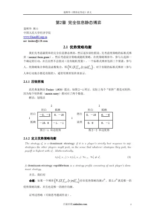
9.2 完全信息静态博弈9.2.1 博弈的战略式表述Definition A normal (strategic) form game G consists of: (1) a finite set of agent s . {1,2,,}D n = (2) strategy sets .12,,,n S S S (3) payoff functions . 12:(1,2,,)i n u S S S R i n ⨯⨯⨯→=囚徒B囚徒A完全信息静态博弈是一种最简单的博弈，在这种博弈中，战略和行动是一回事。

博弈分析的目的是预测博弈的均衡结果，即给定每个参与人都是理性的，什么是每个参与人的最优战略？什么是所有参与人的最优战略组合？纳什均衡是完全信息静态博弈解的一般概念，也是所有其他类型博弈解的基本要求。

下面，我们先讨论纳什均衡的特殊情况，然后讨论其一般概念。

9.2.2 占优战略（Dominated Strategies ）均衡一般说来，由于每个参与人的效用（支付）是博弈中所有参与人的战略的函数，因此，每个参与人的最优战略选择依赖于所有其他参与人的战略选择。

但是在一些特殊的博弈中，一个参与人的最优战略可能并不依赖于其他参与人的战略选择。

也就是说，不管其他参与人选择什么战略，他的最优战略是唯一的，这样的最优战略被称为“占优战略”。

Definition Strategy s i is strictly dominated for player i if there is some such that i i s S '∈ for al .(,)(,)i i i i i i u s s u s s --'>i i s S --∈Proposition a rational player will not play a strictly dominated strategy.抵赖 is a dominated strategy. A rational player would therefore never 抵赖. This solves the game since every player will 坦白. Notice that I don't have to know anything about the other player . 囚徒困境：个人理性与集体理性之间的矛盾。

博弈与决策讲义一：绪论Game Theory（结合耶鲁课程）一、博弈论的概念博弈论（Game Theory），有时也称为对策论，或者赛局理论，应用数学的一个分支, 目前在生物学，经济学，国际关系，计算机科学, 政治学，军事战略和其他很多学科都有广泛的应用。

主要研究公式化了的激励结构（游戏或者博弈（Game)）间的相互作用。

是研究具有斗争或竞争性质现象的数学理论和方法。

也是运筹学的一个重要学科。

博弈论考虑游戏中的个体的预测行为和实际行为，并研究它们的优化策略。

表面上不同的相互作用可能表现出相似的激励结构(incentive structure)，所以他们是同一个游戏的特例。

其中一个有名有趣的应用例子是囚徒困境(Prisoner's dilemma)。

博弈论研究策略形势。

经济学中有这样的案例，如完全竞争企业，这些企业是价格的接受者，他们不必担心竞争对手的行为；又比如完全垄断企业，他没有竞争对手，所以这些都不是策略形势。

他们不是价格接受者，但需要面对需求曲线，对于学过经济学的应该不陌生。

而介于这两种情况之间的就是策略形势，不完全竞争情况就是策略形势，比如汽车企业，在汽车产业里，福特关注通用和丰田的行为，可能还得关注克莱斯勒的行为，少数几家公司的决策会相互影响。

策略形势书面定义就是行为影响结果，而结果不仅取决于自己的行为，还取决于其他人的行为。

具有竞争或对抗性质的行为成为博弈行为。

在这类行为中，参加斗争或竞争的各方各自具有不同的目标或利益。

为了达到各自的目标和利益，各方必须考虑对手的各种可能的行动方案，并力图选取对自己最为有利或最为合理的方案。

比如日常生活中的下棋，打牌等。

博弈论就是研究博弈行为中斗争各方是否存在着最合理的行为方案，以及如何找到这个合理的行为方案的数学理论和方法。

生物学家使用博弈理论来理解和预测演化（论）的某些结果。

例如，John Maynard Smith 和George R. Price 在1973年发表于《自然》杂志上的论文中提出的“evolutionarily stable strategy”的这个概念就是使用了博弈理论。