Kinematics of SiO J=8-7 Emission towards the HH 212 Jet

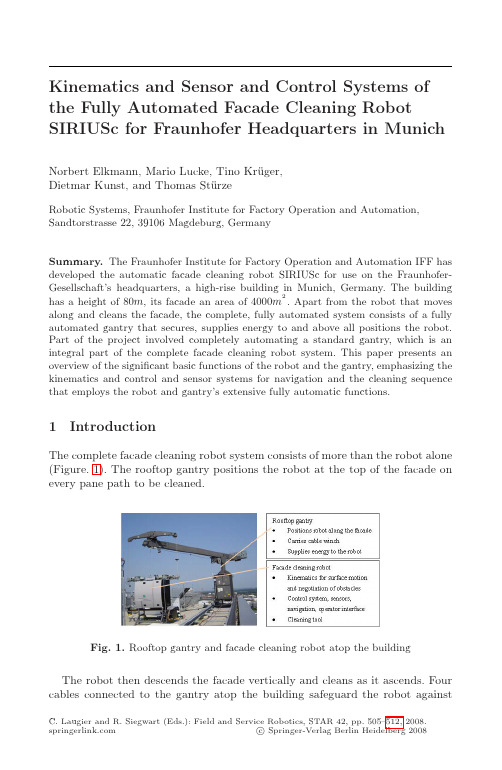
Kinematics and Sensor and Control Systems of the Fully Automated Facade Cleaning Robot SIRIUSc for Fraunhofer Headquarters in Munich Norbert Elkmann,Mario Lucke,Tino Krüger,Dietmar Kunst,and Thomas StürzeRobotic Systems,Fraunhofer Institute for Factory Operation and Automation, Sandtorstrasse22,39106Magdeburg,GermanySummary.The Fraunhofer Institute for Factory Operation and Automation IFF has developed the automatic facade cleaning robot SIRIUSc for use on the Fraunhofer-Gesellschaft’s headquarters,a high-rise building in Munich,Germany.The building has a height of80m,its facade an area of4000m2.Apart from the robot that moves along and cleans the facade,the complete,fully automated system consists of a fully automated gantry that secures,supplies energy to and above all positions the robot. Part of the project involved completely automating a standard gantry,which is an integral part of the complete facade cleaning robot system.This paper presents an overview of the significant basic functions of the robot and the gantry,emphasizing the kinematics and control and sensor systems for navigation and the cleaning sequence that employs the robot and gantry’s extensive fully automatic functions.1IntroductionThe complete facade cleaning robot system consists of more than the robot alone (Figure.1).The rooftop gantry positions the robot at the top of the facade on every pane path to be cleaned.Fig.1.Rooftop gantry and facade cleaning robot atop the building The robot then descends the facade vertically and cleans as it ascends.Four cables connected to the gantry atop the building safeguard the robot against ugier and R.Siegwart(Eds.):Field and Service Robotics,STAR42,pp.505–512,2008. c Springer-Verlag Berlin Heidelberg2008506N.Elkmann et al.falling.Since the cables must be taut to ensure the robot is secure,the cables are also used to position the robot as the winding and unwinding winch on the rooftop gantry moves it vertically along the building and to bear the load of the robot.Cables transmit data and supply power too.The robot is one of thefirst fully automatic systems of this kind used in a public setting.The robot weighs 450kg,the gantry5000kg.2Rooftop Gantry CraneThe gantry(Figure.2)possesses three degrees of freedom relevant for positioning the robot on the facade:Movement along the rails and two rotary cantilever arms.Measuring systems help position the gantry on the roof to start on the pane path to be cleaned.The gantry has two asynchronous drives to move along the rails.Two encoders determine the gantry’s position.The gantry is positioned by a continuous controller that reads the pane path positions taught out of a data module of the control system.Another redundant measuring system has been installed to counteract the slip.Fig.2.Gantry’s degrees of freedom to position and deposit the robot on the facade When the encoder target position is reached,the transponders mounted on each of the pane path target positions must be matched with the transponder system.If the transponder assigned to each pane path can be read out success-fully,the target position has been reached and the positioning of the cantilever arm can begin.Otherwise,an error code is generated and the start on the pane path must be repeated.A synchronous movement of the two rotary cantilever arm drives sets the robot on the facade.To achieve a high level of security when positioning the robot,its orientation parallel to the facade during motion must be guaranteed.A cascaded controller in the gantry control system ensures this.Kinematics and Sensor and Control Systems507 Since the rails execute a curve and do not run parallel to the facade,a par-ticular challenge is positioning the robot and thus the gantry on the corners of the facade.The gantry’s traveling mechanism(translation)and the cantilever arms(rotation)must run sequentially synchronized to prevent any collision of the robot with the facade.The gantry must proceed along the rails to reduce the robot’s distance to the facade and to deposit the robot on it.Simultaneously, this negatively influences the robot’s orientation plane-parallel to the facade.To simplify the positioning process,the traveling mechanism is guided in a second step to the window pane target position and then the cantilever arms are moved again so that the robot reaches its ideal position(a distance of approximately 100mm and parallel to the facade).All operations are fully automated.The gantry is a standard piece of equipment that was completely automated in the project.3SIRIUSc KinematicsAbove all,the modular kinematics(Figure.3)ensures the robot remains in con-stant contact with the facade and can navigate a multitude of typical obstacles and move quickly along a facade.The kinematics is based on a structure of two pairs of linear modules,the so-called"‘advanced sliding module mechanism"’[8,9].Two linear modules constitute one pair that performs the same linear movement,thus ensuring secure and stable contact with the facade.Servo drives move each of the outer or inner sucker units to the next position on a pane within a frame.The linear modules with their suckers are positioned in such a way that the suckers are located above or below the horizontal pane frames when docking onto the facade.Once a sucker unit has suctioned on,the drive’s brake is deactivated and the other unit’s suckers are released and retracted.The winding and unwinding of the securing cables on the gantry lift winch produces the robot’s upward and downward motion on the facade.The alternation of the outer and inner sucker units with2×3suckers apiece produces the robot’s walking motion.As the robot is lifted or lowered to the desired position,the other activated linear module pair is moved to the next free position.Eddy current sensors mounted on the top and bottom of the robot’s body detect and store the positions of horizontal pane frames.One of the requirements for outdoor operation in high winds is that the robot be able to correct its direction of motion,should it drift a bit offcourse.To this end,the inner pair of linear modules is tilt adjustable to enable small steering movements to keep the robot on a straight path.Two drift scanners have been mounted on the robot to control drift compensation.The scanners’job is to detect the robot’s position in relation to pane frames(vertical pane jambs)in order to systematically control the inner linear modules.A drift scanner con-sist of2×4eddy current sensors(spaced50mm),which a controller assembly switches offand on in succession.This is necessary since the eddy current sensors would otherwise interfere with one another.Depending on the robot’s direction of movement and which eddy current sensors detect the metallic pane frames,508N.Elkmann et al.Fig.3.SIRIUSc kinematics and navigation sensorsFig.4.Schematic diagram of the detection of drift variationthe pneumatic drift compensation drive turns the inner linear guide right,to the middle or left.The pane frames are made of various materials and profiles.This represents a special challenge.In extensive testing with various types of sensors,only novel eddy current sensors with a detection distance of0–50mm were sufficientlyKinematics and Sensor and Control Systems509 reliable.None of the optical or other sensors were sufficiently reliable under the given conditions(rain,reflected sunlight on the panes).4Cleaning SequenceFirst,the gantry automatically positions the robot before the facade.Since the rails on the roof and the panes on the facade are not exactly parallel to one another,the robot must be set down supported by two tactile distance sensors mounted on it.In the process,all three of the gantry’s degrees of freedom are controlled.Once the robot is located only100mm in front of the uppermost pane of the facade,four vacuum suckers with a stroke of250mm located on the robot are retracted.After the four suckers have developed a vacuum,the robot is pulled onto the pane and the robot’s vacuum suckers used for moving along the facade establish the robot’s contact to the facade.Fig.5.Robot and cleaning head motion(operation/sequence)on a pane path The robot descends to the bottommost pane(see Section3on page4)and is moved vertically by the cable winch on the gantry,the robot’s suckers al-ways being in contact with the facade.Sensors continuously register the pane frames(horizontal and vertical).Consequently,the direction of the robot’s verti-cal movement is corrected and the walking algorithm is controlled.The walking510N.Elkmann et al.algorithm positions the robot’s linear modules in such a way that the maximum number of suckers is always on the facade and the suckers are always positioned on the panes and not on the frames.Once the bottom pane has been reached, the cleaning head is positioned on the pane to be cleaned(Figure.5).The water cycle and the rotating cleaning brushes are activated.The cleaning head runs sideways until it meets the frame.Tactile sensors on all four sides of the cleaning head detect the pane frames.If the cleaning head has contact with the frame, the robot continues moving downward until the lower pane jamb has also been detected.On the lower pane jamb,the head is moved to the opposite side of the pane,cleaning the pane.Once the head has traveled back and forth one time,the robot moves upward the height of the cleaning head.When the upper pane frame is detected,the cleaning head is run once more laterally,the cleaning water suctioned up and the cleaning head retracted from the pane.When the uppermost pane has been reached and the complete pane path cleaned,the robot disengages from the facade.Once the cleaning of a vertical pane path has concluded,the gantry moves the cleaning robot one pane width laterally.5Control System and NavigationThe heart of the system is its control system,which receives and combines sen-sor data and operator instructions to generate robot actions.Selected for it is stability and modularity,a programmable logic controller(PLC)is used for the robot and the gantry control system.The PLC is on board and controls the en-tire system.It synchronizes the walking mechanism with the trolley and cleaning head.All robot motions and actions are fully automated.The robot was pro-grammed modularly so that it can be transferred to a large number of different facades with minimal reprogramming work.The robot does not start out with information on all the obstacles it will face in its path.Rather,it keeps track of the surface and obstacles currently under it.Sensors identify and measure obsta-cles and window frames.The PLC then generates the appropriate step lengths for the robot to successfully walk over obstacles and frames.The PLC ensures that vacuum suckers directly over an obstacle are not engaged while simulta-neously maximizing the number of vacuum suckers in contact with the facade at any given moment.Like SIRIUS,the cleaning head does not require detailed information on the surface of the facade.Rather,the cleaning system has its own sensors that detect obstacles and end positions.The sensor signals are also incorporated in the onboard PLC program,which in turn uses the information to generate the necessary cleaning head movements.The only manual input information the robot requires before starting offon a given surface is end point data such as the height of the structure or building, offlimit zones and the maximum length of obstacles.The robot automatically detects any other necessary surface information during operation.An operator master display is also located in the building so that an operator can monitor the robot’s progress.A remote maintenance module allows downloading the robot’sKinematics and Sensor and Control Systems511Fig.6.Control system conceptFig.7.SIRIUSc on the high-rise building of the Fraunhofer-Gesellschaft’s headquarters in Munichstatus and sensor data,uploading new program modules and executing simple operator commands such as the motion commands for a pair of linear modules. All this can be done over the Internet.Little knowledge about the general structure of a building’s surface is needed before robot movement can be generated.The input data includes end positions, moving distances and path characteristics.This a priori data is supplemented by online sensors that detect the facade surface and search for possible obstacles.In addition to identifying obstacles,the external sensor technology also corrects the direction of motion.Sensors detect where the robot must deviate from a path, e.g.girders or window and panel seals.The robot control system communicates512N.Elkmann et al.with the building control system,making sure all windows are closed in areas being cleaned.6ConclusionThe Fraunhofer IFF has developed a fully automated facade cleaning robot for the Fraunhofer-Gesellschaft’s headquarters in Munich.Developed for ver-tical facades,SIRIUSc consists of the main components of robots mechanics and kinematics,rooftop gantry,sensor systems to detect facade shape,frames and obstacles,control technology and navigation system,power supply system and integrated cleaning unit.SIRIUSc was delivered to the facility management at the Fraunhofer-Gesellschaft’s headquarters in2006.The facility management staffis now able to clean the facade without any technical support from the researchers at the Fraunhofer IFF.References1.Hirose,S.,Kawabe,K.:Ceiling Walk Climbing Robot Ninja-II.In:Proceedings ofCLAWAR1998,First International Symposium on Mobile,Climbing and Walking Robots,Brussels,October26-28,1998,pp.143–147(1998)2.Cusack,M.M.,Thomas,J.G.:Robotics for the Inspection of Vertical Surfaces ofBuildings and Structures.In:25th ISIR,pp.287–295.3.Elkmann,N.,Felsch,T.,Sack,M.,Boehme,T.:Modular Climbing Robot for Out-door Operations.In:Proceedings of CLAWAR1999.Second International Confer-ence on Climbing and Walking Robots,Portsmouth,September13-15,1999,pp.413–419(1999)4.Elkmann,N.,Felsch,T.,Sack,M.,Boehme,T.,Hortig,J.,Saenz,J.:ModularClimbing Robot for Service Sector Applications.Industrial Robot26(6)(1999) 5.Elkmann,N.,Felsch,T.,Sack,M.,Boehme,T.,Saenz,J.:SIRIUS:Modular Climb-ing Robot for Facade Cleaning and Other Service Jobs.In:International Conference on Field and Service Robotics FSR2001,Helsinki(2001)6.Felsch,T.,Elkmann,N.,Sack,M.,Saenz,J.:Concepts of Service Robots for FacadeCleaning.In:International Symposium on Robotics ISR2001,Seoul(2001)7.Sack,M.,Elkmann,N.,Felsch,T.,Boehme,T.:Intelligent Control of Modular Kine-matics:The Robot Platform SIRIUS.In:International Symposium on Intelligent Control ISIC2002,Vancouver,Canada(2002)8.Elkmann,N.,Felsch,T.,Sack,M.,Saenz,J.,Hortig,J.:Innovative Service RobotSystems for Facade Cleaning of Difficult-to-Access Areas.In:International Confer-ence on Intelligent Robots and Systems IROS2002,Zurich(2002)9.Elkmann,N.,Lucke,M.,Krüger,T.,Kunst, D.,Stürze,T.:SIRIUSc:FullyAutomatic Facade Cleaning Robot for a High-rise Building in Munich.In: ISR/ROBOTIK2006,Munich,Germany(2006)。

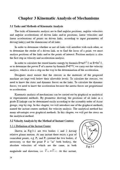
Chapter 3 Kinematic Analysis of Mechanisms3.1 Tasks and Methods of Kinematic AnalysisThe tasks of kinematic analysis are to find angular positions, angular velocities and angular accelerations of driven links and/or positions, linear velocities and linear accelerations of points on driven links, according to input parameters of driving link(s) and the dimensions of all links.In order to determine whether or not all links will interfere with each other, or to determine the stroke of a driven link, or to find the locus of a point, we must analyse positions of the links and/or the points of interest. Position analysis is also the first step in velocity and acceleration analysis.In order to calculate the stored kinetic energy by formula E=mV 2/2 or E=J ω2/2, or to determine the power P of a motor by formula P=F*V , we carry out the velocity analysis, which is also a step on the way to the determination of the acceleration.Designers must ensure that the stresses in the materials of the proposed machine are kept well below their allowable levels. To calculate the stresses, we need to know the static and dynamic forces on the links. To calculate the dynamic forces, we need to know the acceleration because the inertia forces are proportional to acceleration.Kinematic analysis of mechanisms can be carried out by graphical or analytical or experimental methods. By geometric drawing, the positions of all links in a grade II linkage can be determined easily according to the assembly order of Assur groups, step by step. In this chapter, we will introduce one of the graphical methods, named the instant centres method, for velocity analysis. The analytical method has many advantages over graphical methods. In this chapter, we will put the stress on the analytical method.3.2.1 Definition of the Instant CentreShown in Fig.3-1 are two bodies 1 coincident points, e.g. P 1 and P 2necessary, so that the point P is "in" both absolute velocities of which are the magnitude and direction, i.e. V V P P 12=. At this instant,Fig.3-1there is no relative velocity between this pair of coincident points, i.e.V VP P P P1221==0. Thus, at this instant, either link will have pure rotation relative to the other link about the point. This pair of coincident points with the same velocities is defined as the instantaneous centre of relative rotation, or more briefly the instant centre, denoted as P12or P21. If one of links is the frame, the instant centre is called an absolute instant centre, otherwise, a relative instant centre. The absolute instant centre is the zero-velocity point on a moving link, but its acceleration may not be zero.At the position shown in Fig.3-1, the two links rotate relative to each other about the instant centre P12. So any other pair of coincident points, e.g. A1 and A2, will have relative velocities, i.e. V A1A2 and V A2A1. The directions of V A1A2 and V A2A1 are perpendicular to PA. Therefore, if the direction of the relative velocity of a pair of coincident points, e.g. A1 and A2, is known, then the instant centre must lie somewhere on the normal to the relative velocity passing through the coincident point A.3.2.2 Number of Instant Centres of a MechanismEach pair of links i and j has an instant centre and P ij is identical to P ji. Thus the number N of instant centres of a mechanism with K links isNK K=-*()12Note: The frame is included in the number K.3.2.3 Location of the Instant Centre of Two Links Connected by a Kinematic Pair (1) Revolute pairIf two links 1 and 2 are connected by a revolute pair, as shown in Fig.3-2(a), the centre of the revolute pair is obviously the instant centre P12 or P21.(2) Pure-rolling pairThe pure-rolling pair is a special case of a higher pair, as shown in Fig.3-2(b). There is no slipping between the two contacting points A1and A2, i.e. V A1A2=V A2A1=0. Thus the point of contact A is the instant centre P12or P21. Kinematically, the transmission between a pair of gears is equivalent to rolling without slipping between a pair of circles. So the contact point of the two pitch circles of the gears 1 and 2 is the instant centre P12 for the gears 1 and 2, as shown in Fig.3-2(c).(3) Sliding pairAs can be seen in Fig.3-2(d), relative translation is equivalent to relative rotation about a point located at infinity in either direction perpendicular to the guide-way. Therefore, the instant centre of the two links connected by a sliding pair lies at infinity in either direction perpendicular to the guide-way.The instant centres mentioned so far are called observable instant centres and should be located and labeled before any others are found.(4) Higher pair (rolling & sliding pair)Shown in Fig.3-2(e) are two links 1 and 2 connected by a higher pair. Their contact point is point A. The direction of relative velocities, V A1A2and V A2A1, between A1 and A2 must be along the common tangent. Otherwise there will be a relative velocity component along the common normal n-n which will make the. According to the theorem of three centres, the three instant centres P12 , P13 and P23 must lie on a straight line. This theorem can be proved as follows.Suppose that the positions of P12 and P13 are known, as shown in Fig.3-3. Let us consider any point, e.g. point C, outside the line P12P13. Since P12(A) is the instant centre of the links 1 and 2, the link 2 rotates relative to the link 1 about the point A. So V C2C1⊥AC. Similarly, V C3C1⊥BC. Since V C2=V C1+V C2C1, thenV C2C1=V C2-V C1. Similarly, V C3C1=V C3-V C1. Obviously, for any point Coutside the line P12P13, the directions of the vectors V C2C1 and V C3C1 are not thesame, i.e. VC2C1 ≠V C3C1.(V C2-V C1) ≠(V C3-V C1) from which obtains C2≠C3. Hence, according to be the instant centre P 23 between the links 2 and3. In other words, any point outside the straightline P 12P 13 cannot be the instant centre P 23. Thus the theorem of three centres is derived: the three instant centres of any three independent links in general plane motion must lie on a common straight line.3.2.5 Applications of Instant CentresExample 3-1For the four-bar mechanism shown in Fig.3-4, the angular velocity ω1 of crank 1 is given. For the position shown,(1) locate all instant centres for the mechanism,(2) find the ratio ω3 /ω1 of the angular velocity of link 3 to that of link 1,(3) find the velocity V F of point F on link 2.Solution:(1)There are sixcentres in this four-bar mechanism. In order to should first try to locate observable instant centres. There are four instant centres (P 14, P 12, P 23 and P 34) and two unobservable instantcentres (P 13 and P 24) in this mechanism. According to the theorem of three centres, P 13 will lie not only on the line P 14P 34, but also on the line P 12P 23. Since P 23 is at infinity perpendicular to the guiding bar 2, line P 12P 23 passes through the point P 12 Fig.3-3 Fig.3-4and is perpendicular to BF. Hence the intersection E of the lines P14P34 and P12P23 is the instant centre P13.Similarly, line P23P34 passes through the point P34 and is perpendicular to BF, the intersection G of the lines P12P14 and P34P23 is the instant centre P24. Thus it can be seen that it is usual to apply the theorem of three centres twice to determine two lines, the intersection of which will be the unobservable instant centre. Instant centres P14, P34and P24are absolute instant centres, while the others are relative instant centres.(2) In order to find ω3 for the given ω1, we should take advantage of the frame 4. Their three instant centres(P34, P13, P14) lie on a common straight line. The moving links 1 and 3 rotate relative to the frame 4 about the absolute instant centres P14(A) and P34(D) respectively. In link 1, V E1=ω1*L AE. In link 3, V E3=ω3*L DE. (Extend the two links, if necessary, so that the point E is "in" both links.) Since the point E is the instant centre P13between the links 1 and 3, V E1=V E3.Therefore, ω1*L AE=ω3*L DE from which i31=ω3/ω1= L AE/L DE =P14P13/P34P13. The lengths of L AE and L DE are measured directly from the kinematic diagram of the mechanism. The direction of ω3 is counter-clockwise at this instant.From above, it is shown that the ratio ωi /ωj of angular velocities between any two moving links i and j is equal to the inverse ratio of the two distances between the relative instant centre P i j and two absolute instant centres P f i and P f j , that is,ωωijfj ijfi ijP PP P=----------------------------------------------------------------------(3-1)where the subscript f represents the frame! If the relative instant centre P ij lies between the two absolute instant centres P fi and P fj, then the directions of ωi and ωj are different. Otherwise, the directions of ωi and ωj are the same.(3) Since the links 2 and 3 are connected by a sliding pair, they cannot rotate relative to each other. Thus, ω2 =ω3 =ω1*L AE/L ED. Since P24 is the absolute instant centre, the link 2 rotates (relative to the frame 4) about the point P24(G) at this instant. Therefore, V F=ω2*L GF. Its direction is perpendicular to GF, as shown in Fig.3-4. Note: Although the velocity of the point P24(G) is zero, its acceleration is not zero.Example 3-2In the cam mechanism with translating roller follower shown in Fig.3-5, the cam is a circular disk. Supposing that the angular velocity ω1 of the cam is known,the velocity V 2the position shown.Solution: As mentioned in passive DOF. The velocity of change if the roller is welded normal n-n through the point of contact C. Accordingto the theorem of three centres, P 12 must lie on the straight line connecting P 13 and P 23. Since the links 2 and 3 are connected by a sliding pair and their instant centre P 23 is at infinity perpendicular to the guide way, the line P 13P 23 passes through P 13 and is perpendicular to the guide way. Thus the intersection B of the common normal n-n and the line P 13P 23 is the instant centre P 12 and V B1 =V B2. Note: Neither the centre O of the circle nor the contact point C is the instant centre P 12. On the cam 1, V B1 =ω1*L AB . Since the follower 2 is translating, all points on the follower 2 have the same velocity 2. So V 2 =V B2 =V B1 =ω1*L AB .Example 3-3In Fig.3-6, gear 3 rolls onrack 4 without slipping. velocity 1 of slider 1 is velocity V D is to be found.Solution: In order to find the point on the gear 3, angular velocity ω3 of the gear 3 should be found first. As mentioned before, in order to find ω3 of the gear 3 for the given velocity V 1 of the slider 1, we always take advantage of the Fig.3-5 Fig.3-6frame 4. Thus we should try to locate the three instant centres, P34, P14and P13, between the three links 1, 3 and the frame 4. The gear 3 rolls on the fixed rack 4 without slipping. So the contact point C is their instant centre P34. P14 lies at infinity perpendicular to AB(not AC!). P13 must lie on both lines P14P34 and P23P12. So the intersection E of the lines P14P34and P23P12is the instant centre P13between the links 1 and 3. Therefore V E3 =V E1. Since the slider 1 is translating, V1 =V E1 =V E3=ω3*L CE. Thus ω3 =V1/L CE from which V D =ω3*L CD =V1*L CD /L CE. The direction is as shown in Fig.3-6.3.2.6 Advantages and Disadvantages of the Method of Instant CentresThe method of instant centres offers an excellent tool in the velocity analysis of simple mechanisms. However, in a complex mechanism, some instant centres may be difficult to find. In some cases they will lie off the paper. Lastly, it should be pointed out that an instant centre, in general, changes its location on both links during motion. The acceleration of the instant centre is not zero(except for fixed pivots). Therefore, the instant centre method cannot be used in acceleration analysis.3.3 Kinematic Analysis by Analytical MethodsIn graphical methods, none of the information obtained for the first position of the mechanism will be applicable to the second position or to any others. The kinematic diagram of the mechanism must be redrawn for each position of the driver. This is very tedious if a mechanism is to be analyzed for a complete cycle. Furthermore, the accuracy of the graphical solution is limited.In contrast, once the analytical solution is derived using an analytical method, it can be evaluated on a computer for different dimensions and/or at different positions with very little effort. The accuracy of the solution far surpasses that required for mechanical design problems. Thus, in this chapter we will put stress on the analytical method. Graphical methods can be used if necessary as a check on the analytical solutions.There exist many kinds of analytical methods for kinematic analysis of linkages. The kinematic analysis of a multi-bar linkage mechanism seems to be a hard task at first sight. However, it becomes easier if the Assur-group method is used. As mentioned in Sec.2.5, most linkage mechanisms are built up by adding one or more commonly used Assur groups to the basic mechanism. Since the DOF of an Assur group is zero, Assur groups have kinematic determination. That is, the motions of all links in an Assur group can be determined so long as the motions of all outer pairs are known. Taking this fact into account, one can set up subroutinesin advance for some commonly used Assur groups. Then the kinematic analysis of a multi-bar linkage mechanism is reduced to two simple steps: first, dividing the mechanism into Assur groups and secondly, calling the corresponding subroutine for each Assur group according to the type and the assembly order of the Assur group. This method is called the Assur-group method for kinematic analysis.In the next sections, we will set up some commonly used kinematic analysis subroutines before analyzing a six-bar linkage mechanism.3.3.1 The LINK Subroutineand acceleration of a point A (i.e. X A, Y A, (V A)X, (V A)Y(a A)Yacceleration of link AB(i.e. θ, ω, ε) and the length (L ABlink AB are known, as shown in Fig.3-7. The Xcomponents of position, velocity and acceleration of point B (i.e.Fig.3-7X B, Y B, (V B)X, (V B)Y, (a B)X, (a B)Y) can be calculated as follows.In a Cartesian co-ordinate system,X B=X A+L AB * cos(θ) and Y B=Y A+L AB * sin(θ) Differentiating the above position analysis formulae with respect to time, the formulae for velocity analysis can be derived.(V B)X=(V A)X - L AB * sin(θ)*ωand (V B)Y=(V A)Y +L AB*cos(θ)*ωDifferentiating again, the formulae for analyzing the acceleration of the point B can be derived.(a B)X= (a A)X - L AB* sin(θ)*ε - L AB* cos(θ)*ω2and(a B)Y = (a A)Y + L AB* cos(θ)*ε -L AB* sin(θ)*ω2These six formulae can be programmed in a subroutine. In the TRUE BASIC computer language, any subroutine must begin with statement SUB subroutine-name(table of parameters) and end with statement END SUB. Let us name the subroutine LINK. Then the LINK subroutine is as follows:SUB LINK(XA,YA,V AX,V AY,AAX,AAY,Q,W,E,LAB,XB,YB,VBX,VBY,ABX,ABY) LET XB=XA+LAB*COS(Q)LET YB=YA+LAB*SIN(Q)LET VBX=V AX-LAB*SIN(Q)*WLET VBY=V AY+LAB*COS(Q)*WLET ABX=AAX-LAB*SIN(Q)*E-LAB*COS(Q)*W^2LET ABY=AAY+LAB*COS(Q)*E-LAB*SIN(Q)*W^2END SUBEvery evaluating statement must begin with LET. In order to facilitate the understanding of the program, parameters should have easily-recognized names. For example, (V A )X is named V AX. The table of the parameters corresponds to (X A , Y A , (V A )X , (V A )Y , (a A )X , (a A )Y , θ, ω, ε, L AB , X B , Y B , (V B )X , (V B )Y , (a B )X , (a B )Y ). After the subroutine is called, the kinematic parameters of the point B will be known. 3.3.2 The RRR SubroutineIn the RRR group shown inthe kinematic parameters of the points A and C and the lengths of links AB and CB are known. The positions, angular velocities and calculated as follows. When X A , Y A , X C , Y C , L AB determined, there are two assembly modesfor this group, as shown in Fig.3-8, one in solid lines and the other in dashed lines. On the link CB, X B =X C +L CB *cos(θCB ) and Y B =Y C +L CB *sin(θCB )On the link AB, X B =X A +L AB *cos(θAB ) and Y B =Y A +L AB *sin(θAB )Combining these two sets of equations, one obtains:X L X L Y L Y L C CB CB A AB AB CCB CB A AB AB +=++=+⎧⎨⎩*cos()*cos()*sin()*sin()θθθθ ----------------------------(3-2) There are two unknowns, θAB and θCB , in this set of equations. Since there are two assembly modes for this group, there will be two sets of solutions. Although some mathematical skill can be used to solve the above trigonometric non-linear equations to obtain two sets of formulae for θAB and θCB , the calculation process is tedious and the formulae derived would be very complicated. It is hard to judge which set of formulae corresponds to a specific assembly mode. The following is a simple method to overcome this difficulty.(a) L AC =()()X X Y Y C A C A -+-22(b) cos θAC =(X C -X A )/L AC and sin θAC =(Y C -Y A )/L ACThe subroutine may be used for any combinations of the positions of points A Fig.3-8and C. Note that sin θAC may not be equal to ()12-cos θAC since sin θAC may be negative. The magnitude of θAC can be calculated according to the values of both cos θAC and sin θAC by the ANGLE function in TRUE BASIC. Note again that θ may not be equal to ATN(sin θ/cos θ) since θ may be greater than π/2 and less than 3*π/2, whereas the value obtained from the ATN function is only from -π/2 to +π/2. Note: θAC is 180︒ different from θCA .(c) cos θBAC =()()L L L L L AB AC CB AB AC 2222+-/** Since 180︒>θBAC >0︒, sin θBAC =()12-cos θBAC . If L AC >(L AB +L CB ), then cos θBAC >1. This means that the distance L AC between the two outer points is greater than the sum of L AB and L CB . If L AC <|L AB -L CB |, then cos θBAC <(-1) and the distance L AC is less than the difference between L AB and L CB . In these cases, the RRR dyad can not be assembled. The calculation of ()12-cos θBAC will fail and computation will be stopped.(d) As mentioned before, there are two assembly modes for the RRR group. For the assembly mode shown by solid lines, θAB =θAC -θBAC . During motion of the mechanism, the assembly mode does not change as a result of change in position.(e) X B =X A +L AB *cos(θAB ) and Y B =Y A +L AB *sin(θAB )(f) cos θCB =(X B -X C )/L CB and sin θCB =(Y B -Y C )/L CBThe magnitude of θCB can be calculated according to the values of both cos θCB and sin θCB by the ANGLE function in TRUE BASIC.Velocity analysis can be progressed only after the position analysis is finished. The angular velocities, ωAB and ωCB , of the links AB and CB can be found by differentiating Eqs.(3-2) with respect to time. ()*sin()*()*sin()*()*cos()*()*cos()*V L V L V L V L C X CB CB CB A X AB AB AB C YCB CB CB A Y AB AB AB -=-+=+⎧⎨⎩θωθωθωθω -------------(3-3) Both velocity and acceleration equations of a grade II Assur group are dualistic linear equations. The explicit expressions for ωAB and ωCB can be found easily by solving the two equations simultaneously.By differentiating Eqs.(3-3) with respect to time, another set of dualistic linear equations with two unknowns, i.e. the angular accelerations εAB and εCB ofthe links AB and CB, is derived. The explicit expressions for εAB and εCB can be found easily by solving the two equations simultaneously.Using the above explicit expressions, not the equations, the subroutine named RRR for kinematic analysis of the RRR group can be written as follows:SUB RRR(XA, YA, V AX, V AY, AAX, AAY, XC, YC, VCX, VCY, ACX, ACY, LAB, LCB, QAB, WAB, EAB, QCB, WCB, ECB)LET LAC=SQR((XC-XA)^2+(YC-YA)^2)LET COSQAC=(XC-XA)/LACLET SINQAC=(YC-YA)/LACLET QAC=ANGLE(COSQAC,SINQAC)LET COSQBAC=(LAB^2+LAC^2-LCB^2)/(2*LAB*LAC)LET SINQBAC=SQR(1-COSQBAC^2)LET QBAC=ANGLE(COSQBAC,SINQBAC)LET QAB=QAC-QBACLET XB=XA+LAB*COS(QAB)LET YB=YA+LAB*SIN(QAB)LET COSQCB=(XB-XC)/LCBLET SINQCB=(YB-YC)/LCBLET QCB=ANGLE(COSQCB,SINQCB).......................................LET WAB=....................LET WCB=.............................................................LET EAB=.......................LET ECB=.......................END SUBAttention should be paid to the sequence of the revolute's letters in the table of the parameters when the subroutine is called. For this subroutine, the three letters A, B and C are arranged in CCW.3.3.3 The RPR SubroutineShown in Fig.3-9(a) is an RPR Assur group. The revolutes A and C are outer revolute pairs. The eccentric AB is perpendicular to guide-bar BD. The kinematic parameters of the centers, A and C, of the two outer revolute pairs and the length of eccentric AB are known. There are two assembly modes for this group. One is shown in solid lines, the other in dashed lines. The angular position, angular velocity and angular acceleration of the guide-bar BD (θBD, ω, ε) can be calculated as follows:L AC =()()X X Y Y C A C A -+-22, cos θAC =(X C -X A )/L AC ,sin θAC =(Y C -Y A )/L AC ,L BC =L L AC AB 22-.If L AC <L AB , then the group can not be assembled. In this case, the calculation ofL L AC AB 22- will fail and the computation will be stopped.θACB =tg L L AB BC -⎛⎝ ⎫⎭⎪1, θBD = θAC +M* θACB , and θAB = θBD -M*π/2where M is the coefficient of the assembly mode. For the solid mode, M=+1. For the dashed mode, M=-1. During motion of the mechanism, the assembly mode does not change as a result of change in position. We can determine the value of M according to the assembly mode at any angle of the driver.From Fig.3-9, we haveX X L X L L Y Y L Y L L C B BC BD A AB AB BC BD CB BC BD A AB AB BC BD =+=++=+=++⎧⎨⎩cos()cos()cos()sin()sin()sin()θθθθθθ Differentiating the above equations with respect to time results in--+=--+=-⎧⎨⎩()cos()*()()()sin()*()()Y Y VLBC V V X X VLBC V V C A BD C X A XCA BD C Y A Y ωθωθ -------------------(3-4) where VLBC is the derivative of L BC with respect to time.Solving the dualistic linear equations Eqs.(3-4) simultaneously, the explicit(a) (b) Fig.3-9expressions for the two unknowns ω and VLBC can be found.Differentiating Eqs.(3-4) with respect to time (note that VLBC is a variable), another set of dualistic linear equations with two unknowns (one of the unknowns is ε) is derived. The explicit expression for ε can be found easily by solving the two equations simultaneously.The subroutine for the kinematic analysis of the RPR group, which we will name RPR, can be written as follows:SUB RPR(M, XA, YA, V AX, V AY, AAX, AAY, XC, YC, VCX, VCY, ACX, ACY, LAB, QBD, W, E)LET LAC=SQR((XC-XA)^2+(YC-YA)^2)..........................................LET QBD=QAC+M*QACB..........................................LET W=.....................................................................LET E= ..........................END SUBIf L AB=0, then the RPR group in Fig.3-9(a) is simplified into another RPR group shown in Fig.3-9(b). For the RPR group in Fig.3-9(b), L AB=0 and θACB=0. The value of M can be set as any value.Kinematic analysis subroutines for other grade II Assur groups, e.g. RRP, PRP groups in Tab.2-2, can also be derived and established in a similar method. 3.3.4 Main ProgramTo analyze any mechanism, a main program is required. In the main program, suitable kinematic analysis subroutinesAssur groups.Example 3-4The six-bar linkage shown ina constant angular velocity ω1ofknown dimensions of the mechanism are:XX B=41mm, Y B=0, X F=0, Y F=-34m, L ED=14mm, LL BA=28mm, ∠ADC=35︒, L DC=15mm, L FGFig.3-10 program is required to analyze the output motions oflink FG and point G. The mechanism will be analyzed for the whole cycle when thedriver ED rotates from 0︒ to 360︒ with a step size of 5︒.Solution:(a) Group dividingThe composition of this mechanism has been analyzed in Sec.2.5.3. The types and the assembly orders of Assur groups are listed in Table 2-3 of Chapter 2. In this linkage, link ED is the driver. Links 3 and 2 forms an RRR dyad. After this dyad is connected to the driver and the frame, the motion of both links 3 and 2 are determined. Thus we can determine the motion of point C on the link 3. Rocker 4 and block 5 forms a RPR dyad. This dyad can be assembled only after the motion of the point C is determined.(b) Main programThe main program for kinematic analysis of this linkage mechanism can be written as follows:REM The main program for the linkage mechanism in Fig.3-10FOR Q1=0 TO 360 STEP 5CALL LINK(0, 0, 0, 0, 0, 0, Q1*PI/180, 10, 0, 14, XD, YD, VDX, VDY,ADX, ADY)CALL RRR(XD, YD, VDX, VDY, ADX, ADY, 41, 0, 0, 0, 0, 0, 39, 28, Q3, W3, E3, Q2, W2, E2)LET QDC=Q3+35*PI/180CALL LINK(XD YD, VDX, VDY, ADX, ADY, QDC, W3, E3, 15, XC, YC,VCX, VCY, ACX, ACY)CALL RPR(0, 0, -34, 0, 0, 0, 0, XC, YC, VCX, VCY, ACX, ACY, 0, Q4, W4,E4)CALL LINK(0, -34, 0, 0, 0, 0, Q4, W4, E4, 55, XG, YG, VGX, VGY, AGX,AGY)PRINT Q1, Q4*180/PI, W4, E4, XG, YG, VGX, VGY, AGX, AGYNEXT Q1ENDThe subroutine for the first Assur group RRR should be called before that for the second Assur group RPR is called. In the first Assur group RRR, the point D should be a determined point. So we use the first CALL LINK statement to calculate the kinematic parameters of the point D before RRR is called. The parameter PI in the first CALL line is set to πby TRUE BASIC automatically. Emphasis should be put on the assembly mode, the sequence and the correspondence of parameters in the table of parameters when calling a subroutine. Corresponding data are transferred according to the sequence, not according to thename.As mentioned before, an RRR group has two assembly modes, as shown in Fig.3-8. The RRR subroutine is written for the assembly mode shown in solid lines. In order to use the RRR subroutine, the revolutes D, A and B of the RRR dyad in Fig.3-10 must correspond to the revolutes A, B and C of the RRR dyad in Fig.3-8, respectively.In the second Assur group RPR, the revolute centre C should be a determined point. So the second CALL LINK statement must be used to calculate the kinematic parameters of the point C after RRR is called and before RPR is called.The main program ends with the statement END after which all subroutines are listed in any order. Putting the related subroutines(LINK, RRR, RPR) after the END statement of the main program and running it on a computer, produces the3.3.5 Check on the Output DataFaced with a vast amount of digits printed on the screen, it is hard to judge whether or not the output results are correct. The output values from the analytical methods can be checked as follows. For some non-special position of the mechanism, try to draw the kinematic diagram of the linkage mechanism as exactly as possible. Measure the X and Y coordinates of the output points and/or the angular position φ of the output link. Then the measured data are compared with the output position data obtained by the analytical method. Minor differences between the measured values and the analyzed values are acceptable and can be considered as drawing errors and measuring errors. If the output position at the non-special position of the mechanism is correct and the output position data change smoothly during the whole cycle, then the position analysis can be considered to be correct.After the output position data are checked, the output velocity data obtained in the analysis methods can be checked by the instant centers method or by other methods.A simpler way to check output velocity is to examine the qualitative nature of the data. For example, if the displacement is increasing, the corresponding velocity must be positive; otherwise, negative. When the displacement reaches its limit, the corresponding velocity must be zero.Similarly, if the velocity is increasing, the corresponding acceleration must be positive; otherwise, negative. When the velocity reaches its limit, the corresponding。

Kinematics of the 3-UPU wristRaffaele Di Gregorio *Department of Engineering,University of Ferrara,Via Saragat,1,44100Ferrara,ItalyReceived 20September 2000;received in revised form 20May 2002;accepted 19June 2002AbstractRecently,it has been shown that a parallel mechanism architecture,called 3-UPU and used for trans-lational manipulators,can be employed to obtain manipulators able to make the end effector perform infinitesimal spherical motions.The possibility of performing infinitesimal spherical motions is a necessary but not sufficient condition to guarantee that the end effector performs a finite spherical motion,i.e.,the manipulator is a parallel wrist.In this paper it is demonstrated that the 3-UPU architecture,can be em-ployed to obtain parallel wrists,named 3-UPU wrists.Moreover,it is shown that the 3-UPU wrists may reach singular configurations in which the spherical constraint between the end effector and the frame fails.Finally,the singularity condition,that makes it possible to find all the 3-UPU wrist Õs singular configura-tions,is written in explicit form and is geometrically interpreted.Ó2003Elsevier Science Ltd.All rights reserved.Keywords:Manipulators;Parallel mechanisms;Parallel wrists1.IntroductionSpatial parallel manipulators (SPMs)are constituted of an end effector (platform)connected to the frame (base)by a number of kinematic chains (legs).The number of legs usually is equal to the degrees of freedom (dof)of the manipulator and only one actuated joint is present in each leg.By acting on the legs the platform pose (position and orientation)is controlled.Moreover,if the actuators are locked,the manipulator will become an isostatic structure in which all the legs carry the external loads applied to the platform.This SPMs Õfeature makes designing manipulators with high stiffness possible throughout the whole workspace.*Tel.:+39-0532-974828;fax:+39-0532-974870.E-mail address:rdigregorio@ing.unife.it (R.D.Gregorio).0094-114X/03/$-see front matter Ó2003Elsevier Science Ltd.All rights reserved.PII:S0094-114X(02)00066-6Mechanism and Machine Theory 38(2003)253–263In the literature,six dof and less-than-six dof SPMs have been proposed.Among the less-than-six dof SPMs,special attention has been paid to the three dof manipulators since only three dof are necessary in many technical applications.In particular,three dof SPMs which make the platform translate (translational SPMs)[1–8],three dof SPMs which makes the platform perform spherical motion (parallel wrists)[9–13]and three dof SPMs which make the platform perform some special motion neither translational nor spherical [14–17]have been studied.For a long time only two manipulator architectures have been used to obtain parallel wrists.In the first architecture (Fig.1)[11]the platform and the base are joined by a passive spherical pair and the platform orientation is controlled by three legs of type UPS (U,P and S stand for uni-versal joint,prismatic pair and spherical pair,respectively)with the prismatic pair as actuated joint.This parallel wrist has the advantage of being a three dof mechanism and has the drawback of having reduced workspace because of the passive spherical pair.In the second architecture (Fig.2)[9]the platform and the base are connected to each other by three legs of type RRR (R stands for revolute pair)with all the revolute pair axes converging at a fixed point.This parallel wrist is overconstrained and obtains the platform spherical motion by using constraints that are repetitions of other constraints.The overconstrained architecture drawback is that the mechanism jams or high internal loads arise in the links when geometric errors occur.Recently,Karouia and Herv e [13]have sought after the three dof SPMs with three equal legs in which the platform can perform an elementary spherical motion.The capacity of performing an infinitesimal spherical motion is requested,but it is not a sufficient condition to guarantee that the platform performs a finite spherical motion,i.e.,the manipulator is a parallel wrist.Hence their research is only useful to select the architecture that might be parallel wrist.The result of their investigation is that a mechanism architecture,called 3-UPU (Fig.3)and used alreadyfor254R.D.Gregorio /Mechanism and Machine Theory 38(2003)253–263translational manipulators [4],under some mounting and manufacturing conditions,can be used to obtain manipulators able to make the platform perform infinitesimal spherical motions.In the 3-UPU manipulators,the platform and the base are connected to each other by three legs of type UPU in which the prismatic pair is the actuated joint (Fig.3).The mounting and manufacturing conditions enunciated by Karouia and Herv e [13]are as follows (see Fig.4):R.D.Gregorio /Mechanism and Machine Theory 38(2003)253–263255(i)the three revolute pair axes fixed in the platform (base)must converge at a point fixed in the platform (base),(manufacturing condition);(ii)in each leg,the intermediate revolute pair axes must be parallel to each other and perpendicular to the leg axis which is the line through the universal joints Õcenters (manufacturing condition);(iii)the platform Õs point located in the in-tersection of the platform Õs revolute pair axes must coincide with the base Õs point located in the intersection of the base Õs revolute pair axes (mounting condition).Henceforth,a 3-UPU manipulator matching these geometric conditions will be called 3-UPU wrist.The 3-UPU wrist Õs architecture brings about special interest because it overcomes the drawbacks of the two traditional parallel wrists,i.e.,it is not overconstrained and it does not need a passive spherical pair joining platform and base.This paper will demonstrate that the geometric conditions matched by the 3-UPU wrist Õs architecture are sufficient to make the platform perform finite spherical motions when the pris-matic pairs are actuated.Moreover,it will show that the 3-UPU wrists may reach singular configurations (translation singularities)in which the spherical constraint between platform and base fails.Finally,the singularity condition is written in explicit form and is geometrically in-terpreted.2.Finite spherical motion demonstrationFig.4shows a 3-UPU wrist.With reference to Fig.4,the points A i ,i ¼1;2;3,are the centers of the universal joints which connect the legs to the base;the points B i ,i ¼1;2;3,are the centers of the universal joints which connect the legs to the platform and the point P is the common in-tersection of the revolute pair axes fixed in the platform.The 3-UPU wrist is mounted so asto256R.D.Gregorio /Mechanism and Machine Theory 38(2003)253–263make the platform Õs point P coincide with the base Õs point located by the intersection of the re-volute pair axes fixed in the base.Fig.5shows the i th leg,i ¼1;2;3,of the 3-UPU wrist.With reference to Fig.5,w ji ,j ¼1;...;4,is the unit vector of the j th revolute pair axis with the j index increasing from the base to the platform;h ji ,j ¼1;...;4,is the joint coordinate of the j th revolute pair;a i and b i are constant lengths of the segments A i P and B i P respectively;d i is the variable length of the segment A i B i and it is the joint coordinate of the actuated prismatic pair;u i is the unit vector of the leg axis.The point P is fixed in the platform and can be chosen as the origin of a reference system embedded in the platform.The position of P measured in a reference system fixed in the base,locates the platform Õs position with respect to the base.With these notations,by taking into consideration separately the three legs,the platform an-gular velocity,x ,and the velocity,_P,of the point P ,measured in the base,can be written in the following three different ways:x ¼_h1i w 1i þ_h 4i w 4i þð_h 2i þ_h 3i Þw 2i i ¼1;2;3ð1:1Þ_P ¼_B i þx ÂðP ÀB i Þi ¼1;2;3ð1:2Þwhere _h ji ,j ¼1;...;4,are the time derivatives of the joint coordinates h ji ,j ¼1;...;4,respec-tively,and _Bi is the velocity of the platform Õs point B i .Moreover the following vector relationships hold (Fig.5):B i ÀA i ¼d i u ii ¼1;2;3ð2:1ÞP ÀB i ¼b i w 4i i ¼1;2;3ð2:2ÞR.D.Gregorio /Mechanism and Machine Theory 38(2003)253–263257Differentiating relationship(2.1)yields_Bi¼_d i u iþd i_u i i¼1;2;3ð3Þwhere_d i and_u i are the time derivatives of d i and u i respectively.By using the time differentiation rule for constant intensity vectors,the following expression for_u i is obtained(Fig.5): _u i¼ð_h1i w1iþ_h2i w2iÞÂu i i¼1;2;3ð4ÞBy taking into account the relationships(1.1),(2.2),(3),(4),the relationship(1.2)becomes_P¼_diu iþb ið_h2iþ_h3iÞw2iÂw4iþd i_h2i w2iÂu iþ_h1i v i i¼1;2;3ð5Þwherev i¼w1iÂðPÀA iÞi¼1;2;3ð6ÞFinally,the dot product of the i th vector Eq.(5)by w2i yields(Fig.5)_PÁw2i¼_h1i v iÁw2i i¼1;2;3ð7ÞIf the3-UPU mechanism starts moving from rest in a configuration(Figs.4and5)in which the platformÕs point P coincides with the baseÕs point located at the intersection of the baseÕs revolute pair axes,i.e.,the3-UPU wristÕs geometric conditions are matched,then the following additional vector relationships will hold in the initial configuration:w1i¼PÀA ia ii¼1;2;3ð8ÞBy taking into account the relationships(8),the relationships(6)becomev i¼0i¼1;2;3ð9ÞThus,the relationships(7)become_PÁw2i¼0i¼1;2;3ð10ÞSystem(10)is a linear,homogeneous system of three scalar equations in three unknowns:the three components of_P.The matrix form of system(10)isN_P¼0ð11ÞwithN¼½w21;w22;w23 Tð12Þwhere(Á)T indicates the transpose of(Á).If the matrix N is not singular,the homogeneous system (11)will admit only the following solution:_P¼0ð13ÞDifferentiating relationships(7)yields€PÁw2i þ_w2iÁ_P¼€h1i v iÁw2iþ_h1ið_v iÁw2iþv iÁ_w2iÞi¼1;2;3ð14Þ258R.D.Gregorio/Mechanism and Machine Theory38(2003)253–263R.D.Gregorio/Mechanism and Machine Theory38(2003)253–263259 where_v i;_w2i and€h1i are the time derivatives of v i,w2i and_h1i,whereas€P is the acceleration of the platformÕs point P measured in a reference systemfixed in the base.Moreover,differentiating relationship(6)gives_v i¼w1iÂ_P i¼1;2;3ð15ÞIf the3-UPU mechanism assumes a configuration satisfying the3-UPU wristÕs geometric con-ditions(Figs.4and5),the relationships(9)and(13)will hold.Accordingly,in such a case,_v i(see Eq.(15))vanishes and the relationships(14)become€PÁw¼0i¼1;2;3ð16Þ2iEqs.(16)constitute a linear homogeneous system of three equations in three unknowns:the three components of€P.The matrix form of system(16)isN€P¼0ð17Þwhere N is the3Â3matrix given by definition(12).If the matrix N is not singular,system(17)will admit the unique solution€P¼0ð18ÞRelationship(13)and(18)lead to the following conclusion:STATEMENT:If a3-UPU mechanism starts moving from rest in a not singular configuration satisfying the3-UPU wristÕs geometric conditions,it can only perform an infinitesimal motion at the end of which the platformÕs point P still is in the initial position(Eq.(13))and the velocity of P still is zero(Eq.(18)),i.e.,thefinal configuration still satisfies the3-UPU wristÕs geometric conditions and the point P still is at rest.Thus,the next elementary motion also must keep the point P at rest and the3-UPU wristÕs geometric conditions.As a consequence,the platform is bound to perform a sequence of elementary motions keeping the point P at rest,i.e.,the platform is constrained to performfinite spherical motions with center P,until the mechanism reaches a singular configuration.The i th equation of system(10)is the analytic expression of the constraint that the i th leg of type UPU imposes to the platform.With reference to Fig.5,it can be interpreted as follows:a leg of type UPU,with the intermediate revolute pair axes parallel to each other and perpendicular to the leg axis(Fig.5),forbids the displacement along the w2iÕs direction of the platform point(point P in Fig.5)instantaneously coinciding with the intersection of the revolute pair axes at the leg endings.When this point(point P in Fig.5)goes to infinity,i.e.,w1i and w4i(Fig.5)are parallel to each other,the forbidden displacement becomes a forbidden platform rotation around the di-rection of the free vector w2iÂw4i[18].The position analysis of the3-UPU wrist focused on the mechanism configurations that keep the platformÕs point P(Fig.4)at rest is identical with the one of the Innocenti and Parenti-CastelliÕs parallel wrist(Fig.1)[11].Thus,with reference to the demonstration reported in[11],it can be stated that the platform orientations compatible with a given set of values of the three parameters d i,i¼1;2;3,are at most eight,whereas only one triplet of d i values is compatible with a given platform orientation.3.Singularity conditionIn order tofind the3-UPU wristÕs singularity conditions the relationship between the platformÕs velocities,x and_P,and the time derivatives_d i,i¼1;2;3,of the actuated joint coordinates is required.This relationship can be obtained by linearly eliminating the12variables_h1i,_h2i,_h4i,and (_h2iþ_h3i),i¼1;2;3,from the system of18equations composed of the Eqs.(1.1)and(5).By taking into account the relationship(9)and(13),the dot product of the i th Eq.(5)by u i gives the following relationship:ð_h2iþ_h3iÞ¼À_dib i u iÁðw2iÂw4iÞi¼1;2;3ð19ÞOn the other side the dot product of the i th Eq.(1.1)by w2i yieldsw2iÁx¼_h2iþ_h3i i¼1;2;3ð20ÞFinally,substituting the right side of Eq.(19)for(_h2iþ_h3i)into Eq.(20)yieldsw2iÁx¼À_dib i u iÁðw2iÂw4iÞi¼1;2;3ð21ÞThe three Eqs.(21)and the three Eqs.(10)form the following system of six equations:w2iÁx¼À_dib i u iÁðw2iÂw4iÞi¼1;2;3ð22:1Þw2iÁ_P¼0i¼1;2;3ð22:2ÞSystem(22)is the sought-after relationship between the platformÕs velocities,x and_P,and the time derivatives_d i,i¼1;2;3.Since only x appears in Eq.(22.1)and only_P appears in Eq.(22.2),Eqs.(22.1)and(22.2)are decoupled and can be analyzed independently from one another.If the3-UPU wrist assumes a configuration that makes Eq.(22.1)linearly dependent,x will not be determined.The configurations making x indeterminate will be called rotation singularities. If the3-UPU wrist assumes a configuration producing Eq.(22.2)linearly dependent,_P will not be determined,thus the spherical constraint between platform and base fails.The configurations which make_P indeterminate will be called translation singularities.The matrix form of Eq.(22.2)is system(11),whereas the matrix form of Eq.(22.1)is N x¼M_dð23ÞwhereM¼À1b1u1Áðw21Âw41Þ001b2u2Áðw22Âw42Þ001b3u3Áðw23Âw43Þ2666666437777775ð24:1Þ260R.D.Gregorio/Mechanism and Machine Theory38(2003)253–263_d ¼ð_d 1;_d 2;_d 3ÞT ð24:2Þand N is defined by (12).Both system (23)and system (11)are singular when the determinant of matrix N vanishes.Definition (12)of matrix N makes writing its determinant,det(N ),in explicit form possible as followsdet ðN Þ¼w 21Áw 22Âw 23ð25ÞThus,both rotation and translation singularities occur when the configuration assumed by the 3-UPU wrist satisfies the following condition:w 21Áw 22Âw 23¼0ð26ÞSingularity condition (26)will be matched,if the three unit vectors w 2i ,i ¼1;2;3,are linearly dependent,i.e.,they are all parallel to the same plane.From an analytic point of view,the unit vectors w 2i ,i ¼1;2;3,depend on the links Õgeometry and the platform Õs orientation.If the links Õgeometry is given,Eq.(26)will be a scalar equation in the three variables chosen to parameterize the platform Õs orientation.The solutions of a scalar equation in three unknowns lie on a surface,when they are reported in a three-dimensional Cartesian diagram whose coordinates are the three unknown variables of the scalar equation.From a geometric point of view,with reference to Fig.4,condition (26)is verified when the planes the three triangles A i B i P ,i ¼1;2;3,lie on have a straight line through the point P as common intersection (Fig.6).In fact,in this case,the unit vectors w 2i ,i ¼1;2;3,are all per-pendicular to the line common to the three planes and are all parallel to any plane perpendicular to the same line.When this geometric condition occurs,the platform Õs point P can undergo an infinitesimal displacement along the line common to the three planes and the platformcanR.D.Gregorio /Mechanism and Machine Theory 38(2003)253–263261262R.D.Gregorio/Mechanism and Machine Theory38(2003)253–263undergo an infinitesimal rotation around the same line in both of the possible directions after any infinitesimal variation of the lengths d i,i¼1;2;3,is given(Fig.6).A special case of this geometric condition occurs when the three leg axes are all parallel.In sucha situation,the line common to the trianglesÕplanes is parallel to the leg axes.4.ConclusionsIn this paper,it has been shown that a manipulator of type3-UPU,named3-UPU wrist,under some manufacturing and mounting conditions make the end effector performfinite spherical motions after its prismatic pairs are actuated.Moreover,it has been shown that the3-UPU wrist can reach singular configurations,named translational singularities,where the spherical constraint between platform and base fails.Finally,the condition that makes it possible tofind all the3-UPU wristÕs singularities has been written in explicit form and has been geometrically interpreted.AcknowledgementsThefinancial support of the Italian MURST is gratefully acknowledged.References[1]J.M.Herv e,Design of parallel manipulators via the displacement group,in:Proceedings of the9th World Congresson the Theory of Machines and Mechanisms,Milan(Italy),vol.3,1995,pp.2079–2082.[2]R.E.Stamper,L.W.Tsai,G.C.Walsh,Optimization of a three dof translational platform for well-conditionedworkspace,in:Proceedings of IEEE International Conference on Robotics and Automation,1997,paper no.A1-MF-0025.[3]R.Clavel,DELTA:a fast robot with parallel geometry,in:Proceedings of the18th International Symposium onIndustrial Robots,Sydney(Australia),1988,pp.91–100.[4]L.W.Tsai,Kinematics of a three-dof platform with three extensible limbs,in:J.Lenarcic,V.Parenti-Castelli(Eds.),Recent Advances in Robot Kinematics,Kluwer Academic Publishers,Netherlands,1996,pp.401–410. [5]R.Di Gregorio,V.Parenti-Castelli,A translational3-dof parallel manipulator,in:J.Lenarcic,M.L.Husty(Eds.),Advances in Robot Kinematics:Analysis and Control,Kluwer Academic Publishers,Netherlands,1998,pp.49–58.[6]R.Di Gregorio,Closed-form solution of the position analysis of the pure translational3-RUU parallel mechanism,in:Proceedings of the8th Symposium on Mechanisms and Mechanical Transmissions,MTM2000,Timisoara (Romania),2000.[7]P.B.Zobel,P.Di Stefano,T.Raparelli,The design of a3-dof parallel robot with pneumatic drives,in:Proceedingsof the27th Internatinal Symposium on Industrial Robot,Milan(Italy),1996,pp.707–710.[8]R.Clavel,M.Bouri,S.Grousset,M.Thurneysen,A new4d.o.f.parallel robot:the Manta,in:Proceedings of theInt.Workshop on Parallel Kinematic Machines,PKMÕ99,Milan(Italy),1999,pp.95–100.[9]C.M.Gosselin,J.Angeles,The optimum kinematic design of a spherical three-degree-of-freedom parallelmanipulator,ASME Journal of Mechanisms,Transmission and Automation in Design111(2)(1989)202–207.[10]R.I.Alizade,N.R.Tagiyiev,J.Duffy,A forward and reverse displacement analysis of an in-parallel sphericalmanipulator,Mechanism and Machine Theory29(1)(1994)125–137.[11]C.Innocenti,V.Parenti-Castelli,Echelon form solution of direct kinematics for the general fully-parallel sphericalwrist,Mechanism and Machine Theory28(4)(1993)553–561.R.D.Gregorio/Mechanism and Machine Theory38(2003)253–263263 [12]S.K.Agrawal,G.Desmier,S.Li,Fabrication and analysis of a novel3-dof parallel wrist mechanism,ASMEJournal of Mechanical Design117(2A)(1995)343–345.[13]M.Karouia,J.M.Herv e,A three-dof tripod for generating spherical rotation,in:J.Lenarcic,M.M.Stanisic(Eds.),Advances in Robot Kinematics,Kluwer Academic Publishers,Netherlands,2000,pp.395–402.[14]K.-M.Lee,D.K.Shah,Kinematic analysis of a three-degrees-of-freedom in-parallel actuated manipulator,IEEEJournal of Robotics and Automation4(3)(1988)354–360.[15]G.R.Dunlop,T.P.Jones,Position analysis of a3-dof parallel manipulator,Mechanism and Machine Theory34(8)(1997)903–920.[16]M.Ceccarelli,A new3d.o.f.spatial parallel mechanism,Mechanism and Machine Theory32(8)(1997)896–902.[17]R.Di Gregorio,V.Parenti-Castelli,Position analysis in analytical form of the3-PSP mechanism,in:Proceedings of1999ASME Design Engineering Technical Conferences,Las Vegas(Nevada,USA),1999,paper no.DETC99/ DAC-8689.[18]R.Di Gregorio,V.Parenti-Castelli,Mobility analysis of the3-UPU parallel mechanism assembled for a puretranslational motion,in:Proceedings of the1999IEEE/ASME International Conference on Advanced Intelligence Mechatronics,AIMÕ99,Atlanta(Georgia),1999,pp.520–525.。

An improved silicon-oxidation-kinetics and accurateanalytic model of oxidationWang Jimin*,Li Yu,Li RuiweiInstitute of Microelectronics,Tsinghua University,Beijing100084,ChinaReceived26November2001;received in revised form28October2002AbstractThe silicon-oxidation-kinetics of Deal–Grove has been improved.A novel physics model propounds a conception of reaction layer lying between oxide and silicon when the oxidation is going.The reaction is not only at the surface of silicon,as the model of Deal–Grove,but in the whole reaction layer.After the oxidation stopped the reaction layer will become a transition layer.An accurate analytic model of oxidation has been developed.It made of items,linear, parabola and logarithm.Of which,the factors are a,b,c and characteristic width d.In general,ad¼c.In the area of 1–3000nm,the new modelfits very well with the experimental data.The paper explains the reactive rate of oxidation is of extreme lager in the ing the new model can get the width of transition area.The paper offers some model parameter tables and offers the relationship curves between the parameters and oxidation temperature.Ó2003Elsevier Ltd.All rights reserved.Keywords:Oxidation;Kinetics;Modeling;Parameter;Transition1.IntroductionDeal and Grove[1]propounded the thermal oxida-tion kinetics of silicon in1965.As we know,the mixed equation including the linear and parabola is widely used.But the equation does not agree with the experi-mental result of the thin oxide grown by dry oxidation, and we can say it cannot be used to describe the whole process of the dry oxidation directly.In addition,if the temperature of vapor oxidation is higher than1000°C, the model given in literature[1]does not agree well with the experimental result.Massoud[5]revised the model of Deal–Grove.He added a correction item R th in basic equation and offered the parameters used in R th.The corrected oxidation equation can be used to calculate the thin layer of oxi-dation under500 A.In this way,the modeling of dry oxidation is required to treat in subsections.In practice,the models used to simulate the thermal oxidation of silicon[2]are very complex,such as ERFC [3],compress and viscous[4].Those are analytic or nu-merical models and one-dimension or multi-dimension models.But they are all developed from the Deal–Grove model.Wolters and Zeers-Van Duijnhoven offered the ionic growth model[6]with electricfield-dependent ionic conduction.In the analytic equation of the model,the linear item,AX is replaced by the AX2Àa.The equation is afitting power-parabola law and is better agreed with the thin oxide.In the model of Deal and Grove,it assumes that the oxidation reaction occurs at the surface of silicon with a supposed constant oxidation rate.This way can lead to the problem in thin oxide.This paper further analyses the reaction near the interface of the oxide and silicon, to perfect the physical model of Deal and Grove.Then, we will establish the new analytic model and extract the parameter of the model.*Corresponding author.Fax:+8610-62771130.E-mail addresses:wangjm@(W. Jimin),leeyu99@(L.Yu),lirw@tsinghua.(L.Ruiwei).0038-1101/$-see front matterÓ2003Elsevier Ltd.All rights reserved.doi:10.1016/S0038-1101(03)00135-7Solid-State Electronics47(2003)1699–17052.Theory analysisBased on the thermal oxidation kinetics of Deal–Grove,the mixed equation of thermal oxidation model including linear and parabola,isd2oxþAd ox¼BðtþsÞð1Þd ox is the thickness of oxidation layer,t is the time of oxidation,B is the factor of parabola,B=A is called as linear factor,A is the factor of linear item,s is time of initial oxidation.In the dry oxidation,due to s¼0,Eq.(1)cannotfit with the thin-layer-oxide process.Other-wise,in the vapor oxidation with the oxidation tem-perature T>1000°C,Eq.(1)does not agree well with the experimental curve.Now,we restudy the model of the oxidation kinetics.The following three equations given by Deal and Grove are the basic relation of the oxidation kinetics: F1¼hðCÃÀC0Þð2ÞF2¼DðC0ÀC iÞd oxð3ÞF3¼k s C ið4ÞF1is theflux with which the oxidantflows into the surface of oxide from total airflow.F2is theflux of the oxidant thatflows into the silicon across the oxide.F3is theflux been reacted with the silicon at the Si–SiO2in-terface,and the h is gas-state mass transfer coefficient indicated by using the concentration in solid.C0is the balanced concentration of oxidant in the outside surface of oxidation layer.CÃis the balanced concentration in oxide.D is the diffusion coefficient of the oxidant in the oxide.C i is the oxidant concentration in the oxide near the interface of the oxide and silicon.d ox is the thickness of oxide.k s is the rate constant of chemical reaction in the surface of silicon in oxidizing.Fig.1is an improved sketch of the oxidation physical model.It is different from the model of Deal and Grove. It assumes there is an oxidation reaction layer with certain width lying between oxide and silicon.The oxidation is a process in which the diffusion of oxidant and oxidation occur in the same time.In the beginning oxidant,out of silicon surface,diffuses into the silicon and theflux is F1.The oxidant in silicon forms a distribution of concentration from maximum to zero in the region of width w r.We call this region a reaction region in which the part near the surface will complete the oxidationfirstly and form the SiO2region with the thickness of d0.As the time is passing,d0will be larger and larger and the reaction region will boost in the di-rection of silicon.As Fig.1shows,the thickness of the oxide layer can be expressed as d ox¼d0þw r or as the following:d ox¼d01þw rd0ð5ÞIn above equation,w r=d0is the contribution of the width of reaction region to the thickness of the total oxidation layer.We define the c¼w r=d0.Here,c is called as effect factor of the reaction region.When oxidation starts,a great deal of oxidant diffuses into the silicon rapidly and forms the reaction region.The diffusion rate can be calculated and the growth rate of oxidation layer is far slower than diffusion.If d ox!0,then c!1,it will affect the growth of oxidation layer extremely.With the d ox and d0increasing,so theflux of oxidant is decreasing, the rate of diffusion reduces too and c will be less and less.When d ox is so large that c!0it does not affect the growth of the oxidation layer.In this way,it is assumed that the effect factor c of reaction region has approxi-mately the inverse ratio with the width of the total ox-idation layer d ox.If the proportion constant is called d, then,it has the following relation:c¼dd oxð6ÞUnder the specified oxidation condition,in Eq.(6)d is a constant and is called characteristic width.The thickness of the oxidation layer d ox can be expressed with Eq.(7): d ox¼d0ð1þcÞð7ÞFrom Eqs.(5)–(7),the relationship between the reaction region width w r and the oxide thickness d ox can be ex-pressed as following:W r¼dÁd oxd oxþdð8ÞAbove equation shows that if d ox¼0,w r¼0.If d ox¼d, w r¼d ox=2.If d ox!1,w r!d.This shows that char-acteristic width d is equal to the thickness of the total oxide layer if d0¼w r and/or,d is equal to the width of the reaction region,if d ox!1.According to Fig.1,we use the d0instead of d ox in Eq.(3).Then we can get the newflux F2from Eq.(7):F2¼DðC0ÀC iÞD oxð1þcÞð9ÞSame as Eq.(4),it is assumed that theflux of oxidant flowing into the reaction region is direct proportion to C i.The proportion factor is the reaction rate k r in the reaction layer,but is not the surface rate.In the reaction layer,if the oxidation rate is more largely,the oxidant concentration decreases faster and the w r is smaller.Their relation can be approximately written as k r¼k=w r.k is the proportion factor.If k s in Eq.(4)is replaced by k r, from Eqs.(4)and(6),we can obtain Eq.(10):F3¼C i K rLð1þcÞð10ÞHere,k rL¼k=d and k rL is a limitation oxidation rate,if d ox!1.In the steady state,F1¼F2¼F3and from Eqs.(2),(6),(7),(9)and(10),we can derive the fol-lowing equation:N i d d oxd t¼CÃd oxk rLðd oxþdÞþ1hþd2oxDðd oxþdÞð11ÞThe N i is the number of the oxidant molecule that has entered into the unit volume oxide.From Eq.(11)we can get Eq.(12):d2 ox þad oxÀc ln1þd oxd¼btð12ÞThe analytic equation(12)is comprised of parabola, linear and logarithm items with four model parameters. The d is the characteristic width.Parameters a,b and c are the followings:a¼2D1k rLþ1hÀ2dð13Þb¼2DCÃið14Þc¼2Ddk rLÀ2d2ð15ÞEqs.(13)and(15)show that the value of a and c can be minus.When2D=h(a there is following expression:d¼cor ad¼cð16ÞThus Eq.(12)has only three independent parameters:a, b,d or b,c,d.When d ox)d,the logarithm item of Eq.(12)can be ignored,and if d ox)a,we haved2ox¼btð17ÞLet us substitute b in Eq.(17)by Eq.(14)to get fol-lowing:d2ox¼2DCÃN itð18ÞWhen d ox is large enough,Eqs.(17)and(18)are the parabolic law relationship.They are expressed by the model parameters or the physical parameters and are same as the equations of Deal and Grove.When d ox(d,Eq.(12)can be simplified into the following equation:d ox d oxþaÀcd¼btð19ÞIf d ox(ðaÀc=dÞ,we substitute a,b and c of Eq.(19) by Eqs.(13)–(15)to simplify Eq.(19)as following:d ox¼hCÃN itð20ÞWhen d ox is small enough,Eq.(20)is the linear relation of oxide thickness with time of oxidation.The linear factor is different from that of Deal–Grove.It can be expressed as the following equation:k L¼hCÃN ið21ÞThe above equation shows that k L has a direct propor-tion with hCÃ.We can know from Eq.(2),the hCÃis the maximumflux of the oxidantflowing into the surface of oxide from total airflow.Thus,the reaction rate is very larger at beginning moment of the oxidation.At a specified condition of oxidation,if we have four groups of oxidation timeðt1;t2;t3;t4Þand of corre-sponding oxide thicknessðd ox1;d ox2;d ox3;d ox4Þ,by using Eq.(12),we can extract a group of the model parameters with this condition.3.ExperimentThis paper uses the experimental data issued by Technology Associates Company in1982[7].We extract and optimize the model parameters in the process of dry and wet oxidation for h111i and h100i silicon.Table1shows the model parameters of dry oxidation for h111i silicon with different oxidation temperatures.Fig.2shows the relation curves of model parameters and oxidation temperature shown in Table1.The X-axisTable1The model parameters of dry oxidation for h111i siliconT(°C)a(l m)b(l m2/h)c(l m2)d(l m) 8000.1980.00080.001880.0103 9000.450.005080.01380.0326 10000.7580.01930.05590.0773 11000.6590.03720.1330.207 12000.4550.05970.1740.388W.Jimin et al./Solid-State Electronics47(2003)1699–17051701is1000=T and T is the absolute temperature.The sym-bols are the model parameters given in Table1and solid lines are thefitting curves of model parameters.There are b and b=a curve,another is both of d and c=a,see Eq.(16).In Fig.2,d and b=a have the logarithm relation vs. oxidation temperature.From T¼1000°C,b is divided into two segments with different logarithm relations. Thus,we can respectively express the curves of d,b1,b2 and b=a by Eq.(22):n¼C0expðÀE a=kTÞð22ÞHere,n indicates thefitting curves of d,b1,b2and b=a. C0is the coefficient,E a is the activation energy,k is the Boltzmann constant,T is the absolute temperature.Fig. 2provides three groups offitting curve;they all can be described with Eq.(22).The b is divided into two seg-ments from1000°C.Table2lists the values of C0and E a used in Eq.(22) of dry oxidation for h111i silicon,see Fig.2.Fig.3shows the comparison of the experimental curves and the theoretic data they are calculated using Eq.(12)and Table1.The curve L is experimental curve; the M is theoretic data.They agree with each other very well in the experimental range of oxidation temperature T¼800–1200°C and the thickness of d ox¼3–3000nm. The dashed N in Fig.3shows a curve calculated by using the equation of Deal and Grove with the oxidation temperature of1000°C.Obviously,between the theory and the experiment;the larger error can be found when the oxide is thinner.Table3shows the parameters of the oxidation model for h111i silicon with the vapor pressure P¼640s and with the temperature range T¼800–1000°C.In Table3,there are six groups of the model data with different oxidation temperature.The parameters a and c are negative when T¼1200°C.Fig.4shows the curves of model parameters vs.ox-idation temperature which is drawn according to Table3 with a0¼aþ0:5and c0¼cþ0:5.Obviously,the each model parameter has a break between880–900°C,and the values of some parameters are negative.We cannot simply express the relation of the model parameters and oxidation temperature by Eq.(22),but it can be dealt in several segments.Fig.5shows the comparison of the experimental curves and theoretic data of the vapor oxidation for h111i silicon.The L is experimental curves.The M is theoretic data,which is calculated by using Table4and Eq.(12).Obviously,they are agreed very well in the range of the oxidation time1–1000min.The dashed N is the theoretic curve from Eq.(1)of Deal and Grove at the1200°C.For thinner oxide layer the error is larger.The curves in Fig.5show that the oxidation rate has a larger change near the900°C.This agrees with the break of model parameter curves near900°C in Fig.4.Table3Model parameters of vapor oxidation for h111i siliconT(°C)a(l m)b(l m2/h)c(l m2)d(l m)800 1.810.07630.01060.00874880 1.170.1140.01240.0165900 1.920.2820.06960.049410000.5890.350.03450.063811000.16880.52170.009590.09551200)0.3260.554)0.2060.604Table2The values of C0and E a of dry oxidation for h111i siliconC0E a(eV)d(l m)7.086·103 1.2425b=a(l m/h) 1.1496·103 1.166b1(l m2/h) 5.458·105 1.877b2(l m2/h)83.1790.91691702W.Jimin et al./Solid-State Electronics47(2003)1699–1705As similar as Table1,Table4shows the model parameters of dry oxidation for h100i silicon.As similar as Fig.2,Fig.6shows the relation curves of the model parameters in Table4vs.the oxidation temperature.In those,the dashed lines are parameter curves of d,b=a,b and the solid lines are thefitting curves of them.For dry oxidation and h100i silicon,Fig.6shows that,with oxidation temperature T above1000°C,the conformability of model parameters turns worse.The fitting curves can be described by Eq.(22)and its parameters are shown in Table5.As above statement,the oxidation reaction does in the reaction layer.The reaction layer is not perfect oxide.After the oxidation stopped,the reaction region will become the transition region with thickness w r lying between the silicon and the perfect oxide layer.Fig.7is drawn based on Eqs.(6)and(7)and shows the relation curves of the width w r of transition region and the thickness d ox of entire oxide layer with different oxida-tion temperatures.Obviously,the w r will be largerwithTable5The values of C0and E a of dry oxidation for h100i siliconC0E a(eV)d(l m) 1.315·104 1.44624b=a(l m/h) 5.488·103 1.28149b1(l m2/h) 2.877·108 2.57198b2(l m2/h)1360.98213Table4The model parameter of dry oxidation for h100i siliconT(°C)a(l m)b(l m2/h)c(l m2)d(l m)8000.09890.000230.000550.0069000.3870.002910.006110.017210000.8950.01770.03840.046211000.3670.03340.01920.055712000.4550.05970.1740.388the thickness of the oxide layer increasing,and finally,it ends up with w r !d .When the oxidation temperature decreases,the transition region will be thinner.After the oxidation stopped,Fig.8shows a typical oxidation structure,the original reaction layer turn into the transition region.Fig.8shows that the oxidation is a process involved the oxidant diffusion and oxidation reaction.The curves of SiO 2and Si are wt.%per unit volume in the different regions.The oxidant flux F N ¼F 2=F 0is a normalized flux.Here the F 0is the flux with which the oxidant flows from total gas into oxide when its thickness is d ox !0.In the reaction layer,the wt.%of SiO 2decrease from 100down to zero,but the Si increase from zero up to 100gradually.The oxidant flux decreases down to zero in the Si substrate.Because of the oxidation reaction will occur only at where the oxidant have arrived firstly by diffusion.By Eq.(10),F 3is the total flux flowed into the reaction layer,where the oxidation rate is the k r ¼k rL ð1þd =d ox Þ,and will decrease along with the d ox increase,however,there are different rates at the differ-ent sites in the x direction.If we assume the oxidation rate is direct proportion to the product of the oxidant and the Si components.The maximum rate will be edge of transition near the Si substrate.Table 6shows the model parameters of vapor oxi-dation for h 100i silicon.4.DiscussionUsing the analytic model equations and the model parameters in this paper,the result can be obtained that the agreement with the experimental data is very well in a usual range of oxidation time and thickness.But some model parameters have a little scattering to the tem-perature.For dry oxidation process,the conformability of h 111i silicon is the best,but for h 100i silicon,it is not so if oxidation temperature is over 1000°C.For the vapor oxidation,the conformability is a little worse.But it needs to point out that the abnormality of model parameters is agreed with the experimental curves.In general,the model parameters a ,c and d satisfy the condition of Eq.(16)and the analytic model Eq.(12)turns into the equation that includes only three inde-pendent parameters a ,b ,d ,or c ,b ,d .In the dry oxi-dation,the relation is well satisfied,but in the vapor oxidation,it has a little difference.Fig.7provides the basic theoretic relation of width of transition region and thickness of oxide.5.ConclusionThe mixed relation equation comprised of linear,parabola and logarithm items can better describe the oxidation of the silicon than previous model.The model parameters extracted from experimental data,which are optimized,can be used to calculate the oxidation curve.In the whole experimental range being independent of whether thin or thick oxidation layer,it can very well achieve congruity with the experimental data.The new model can be used to estimate the width of transition region.New physical model and analytic model are more perfect.Appendix AAccording to Deal–Grove model,there are three equations of the oxidant flux:F 1¼h ðC ÃÀC 0ÞF 2¼D ðC 0ÀC i Þd oxF 3¼k s C iIn the new model of this paper,there are three equations of the oxidant flux too,as followings:F 1¼h ðC ÃÀC 0ÞTable 6The model parameter of vapor oxidation for h 100i silicon T (°C)a (l m)b (l m 2/h)c (l m 2)d (l m)800 1.0250.03420.00320.00472880 1.6960.1040.01820.0167900 1.7010.1920.0380.036310000.620.3180.00530.01111000.1430.450.00450.07511200)0.3260.554)0.2060.6041704W.Jimin et al./Solid-State Electronics 47(2003)1699–1705F2¼DðC0ÀC iÞd oxð1þcÞF3¼C i k rLð1þcÞNow,we have three comparisons in both relativefluxes of the two models respectively,and wefind that,1.The F1has no changing any thing in the both models.2.For the F2,the d ox is replaced by d ox=ð1þcÞ,in thenew model,and c¼d=d ox,due to here the F2is theflux only in the SiO2layer that does not include the reaction layer.3.For the F3,the surface reaction rate k s is replaced byk rLð1þcÞin the new model.Now,in the steady state,we have F1¼F2¼F3.By the simply algebra operation as that of Deal–Grove,we have following:F3¼CÃ1k rLð1þcÞþ1hþd oxDð1þcÞAnd c¼d=d ox,then,there is following:F3¼CÃd oxk rLðd oxþdÞþ1hþd oxDðd oxþdÞWe suppose,the following equation is of right too in the new model:N i d d oxd t¼F3Then we can obtain Eq.(11)in the paper as following:N i d d oxd t¼CÃd oxk rLðd oxþdÞþ1hþdoxDðd oxþdÞð11ÞTofind the relationship between the thickness and time of the oxidation,we solve Eq.(11)with the boundary condition of that if t¼0,then,d ox¼0.Z d ox 0d oxk rLðd oxþdÞþ1hþd2oxDðd oxþdÞd d ox¼Z tCÃN id tFor simplifying derivation,replacing the d ox by x,there isZ x 0xk rLðxþdÞþ1hþx2DðxþdÞd x¼Z tCÃN id tAccording to the standard integral formulas,there are followings:Z x 0xk rLðxþdÞd x¼1k rLxÀd ln1þxdZ xx2DðxþdÞd x¼1D12x2Àdxþd2ln1þxdZ x1d x¼x;Z tCÃid t¼CÃit andCÃN it¼1k rLxÀd ln1þxdþ1D12x2Àdxþd2ln1þxdþxhWe replace back the x by the d ox,then,there is a equa-tion as following:2DCÃt¼d2oxþ2D1rLþ1À2dd oxÀ2Ddk rLÀ2d2Áln1þd oxdWe can write above equation asd2oxþad oxÀcÁln1þd ox¼btThen,that is Eq.(12)of this paper.There area¼2D1k rLþ1hÀ2dð13Þb¼2DCÃN ið14Þc¼2DdrLÀ2d2ð15ÞReferences[1]Deal BE,Grove AS.General relationship for thermaloxidation of silicon.J Appl phys1965;36:3770.[2]ATHENA userÕs manual,SILVACO International Inc.;April1997.[3]Guillemot N.A new analytical model of the birdÕs beak.IEEE Trans1987;ED-34(5).[4]Chen D.Two dimension oxidation modeling and applica-tions.PhD thesis,Department of Electrical Engineering,Stanford University,June1983.[5]Massoud HZ.Thermal oxidation of silicon in dry oxygengrowth kinetics and charge characteristicization in the thinregime.Technical Report,Stanford Electronic Laboratories,Stanford University,June1983.[6]Wolters DR,Zeers-Van Duijnhoven ATA.Advanced mod-eling of silicon oxidation.Microelectron Reliab1998;38(2):259–64.[7]Semiconductor technology handbook.2nd ed.TechnologyAssociates Inc.;1982.W.Jimin et al./Solid-State Electronics47(2003)1699–17051705。