abaqus屈曲分析实例_New

基于ABAQUS复合材料薄壁圆筒的屈曲分析由于玻璃钢复合材料的薄壁圆筒结构具有强度高、重量轻、刚度大、耐腐蚀，电绝缘及透微波等优点，目前已广泛应用于航空航天和民用领域中。

工程中广泛使用的这些薄壁圆筒，当它们受压缩、剪切、弯曲和扭转等荷载作用时，最常见的失效模式为屈曲。

因此，为了保证结构的安全，需要进行屈曲分析。

对结构进行屈曲分析，涉及到较复杂的弹(塑)性理论和数学计算，要通过求解高阶偏微分方程组，才能求解失稳临界荷载，而且只有少数简单结构才能求得精确的解析解。

因此，只能采用能量法、数值方法和有限元方法等近似的分析方法进行分析。

近20年来，随着计算机和有限元方法的迅猛发展，形成了许多的实用分析程序，提高了对复杂结构进行屈曲分析的能力和设计水平。

ABAQUS 就是其中的杰出代表。

1.屈曲有限元理论有限元方法中，对结构的屈曲失稳问题的分析方法主要有两类：一类是通过特征值分析计算屈曲载荷，另一类是利用结合Newton—Raphson迭代的弧长法来确定加载方向，追踪失稳路径的几何非线性分析方法，能有效分析高度非线性屈曲和后屈曲问题。

1.1线性屈曲假设结构受到的外载荷模式为P0。

，幅值大小为λ，结构内力为Q，则静力平衡方程应为λP0=λQ进一步考察结构在(λ+△λ)P0载荷作用下的平衡方程，得到{[K E]+[K S(S+λ△S)]+[K G(ũ+λũ)]}△ũ=△λP0由于结构达到保持稳定的临界载荷时有△λ，代入上式得{[K E]+λ[K S△σ]+K G(△ũ)}△ũ=0该方程对应的特征值问题为det{[K E]+λ[K S△σ]+K G(△ũ)}=0如果忽略几何刚度增量的影响，屈曲分析的方程又可进一步简化为det{[K E]+λ[K S△σ]}=0该方程即为求解线性屈曲的特征值方程。

λ为屈曲失稳载荷因子，(△ũ)为结构失稳形态的特征向量。

1.2非线性屈曲非线性屈曲分析方法多采用弧长法进行分步迭代计算，在增量非线性有限元分析中，沿着平衡路径迭代位移增量的大小(也叫弧长)和方向，确定载荷增量的自动加载方案，可用于高度非线性的屈曲失稳问题。

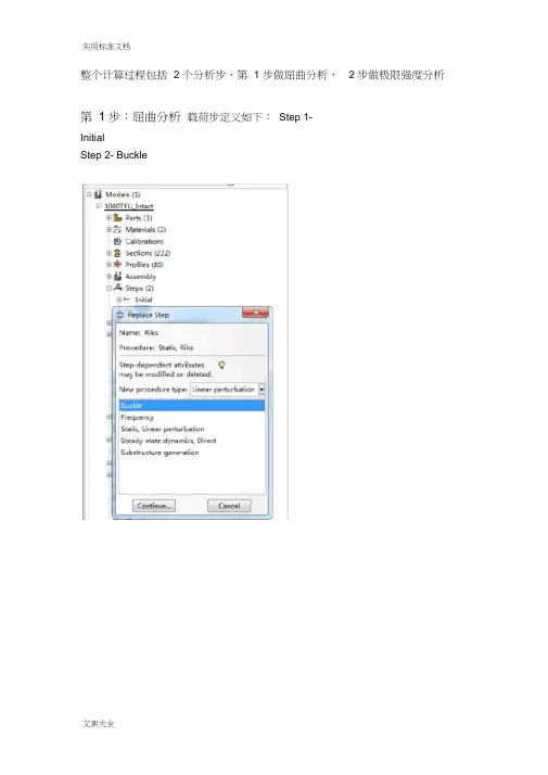
实用标准文档整个计算过程包括 2 个分析步，第 1 步做屈曲分析，第 1 步：屈曲分析载荷步定义如下：Step 1-InitialStep 2- Buckle2 步做极限强度分析0奪莖UWICWHIK . 叽I J I*' *iirl |U*ii:* ri«-2- c.仲［U**t Wfl| «R =・|0T* |«|M4 11 屮W Ml 町扌垮・3 4M4; *E>|轴亠白*wr»44* «*M *A*S MMM-in 4414-* Ita1! I >H*d *■.■ Lrfi|i-t*b*i UWi^ *4」>jU***^ ::切2冲<a：K-.L口sMwSniLpc^l Efl «o 誓光n-3 wa HF HB・・n c:^ > q士* f *B£ -A <MI '■■*W■uTp*』«MLrii4 *M；■pofit ■直j.i t…叫町■ ' H.,机...i . r |fl»-L , | |-£I -t fr E叶*盅1并在Model-Edit Keywords 的图中位置加入下面的文字，输出屈曲模态*nodefile, global=yesU,Create job 名称为“ Buckling点击continue ，完成第 1 步的计算第 2 步：极限强度分析将“ buckle ”分析步替换为“ riks ”分析步在Basic 选项卡中，Nlgeom：选择打开在Instrumentation 选项卡中，定义如下参数，然后点击OK Array定义一个新计算工作，输入名称，点击continue在Parallelization 选项卡，选择 2 个CPU，如下所示，点击OK。

在此编辑Model-edit keywords ，删除“第 1 步”加入的文字“ *nodefile, global=yesU,”，并在下图位置加入下段文字：*imperfection, file=buckling, step=1 1, 2.5点击OK，再保存文件最后提交计算。

Eigenvalue buckling and Elastic buckling stress analysis of Simply Supported Rectangular Plate Uniformly Compressed in One Directionby using ABAQUS1. Double click Abaqus CAE on desktop or click start → programs → abaqus 6.7-4 →abacus CAE.2. Display of the abaqus 6.7-4 menuTo begin a new model, click Create Model Database, and the display is shown as:3. Double click icon and appear Create Part dialog box:In this dialog box, change Name Part-1 with plate (example only), in shape column select Shell and in the column type select Planar. Approximate size is given by 3000 (example only), and click Continue.4. Click icon to draw rectangular plate is shown as:5. Click icon to add dimension, select the line and fill dimension of plate 2400 forplate length also 800 for plate breadth (example only) into new dimension dialog box and press enter.And than click to fix the display. In display, right click on mouse click cancel procedure and click done is shown as6. Double click to define material is shown as:In this dialog box change name Material-1 with steel (example only) and select Elastic and appear dialog box is as shown:7. Double click to create section is as describe;In this figure, change Name: Section-1 with plate (example only), select shell in category column and select Homogeneous in type column, afterwards clicks continue. Also fill the Shell thickness with 10 and click OK.8. In the figure below, select Parts → plate →double click Section Assignments → andAnd click OK inthe Edit SectionAssignmentdialog box.9. From Parts → plate →double click Mesh (Empty). Afterwards, select Seed and clickPart is as shown by figure;Fill approximate global size 50 and clickOKSelect Mesh from menu bar and In Mesh Controls dialog box selectControls Structured and click OKFrom menu bar click Mesh and and click YesSelect Part10. Click Assembly double click Instances. In the Create Instance dialog box click onAuto-offset from other instances and click OK.11. Double click Steps (1) and appear Create Step dialog box. Afterwards, Name: Step-1 is changed by load (example only), Procedure type: Linear perturbation. SelectBuckle and click Continue.Fill in Number of eigenvalues requested: 10 (example only) and click OK12. Double click Loads, select Shell edge load and click ContinueSelect the left edge of the plate, and click doneIn the Edit Load dialog Box fill inMagnitude 0.01and click OK and load willapply on plate is shown as in figure:Name: BC-1 (example only can be changed or not) and click continue.Select the edge and click done. Afterwards, Edit Boundary Condition dialog box will appear and make sign . In this case, U3, UR1 and UR3 are fixed (can not move and rotate) and click OK. Similarly for the three edges of the plate.After completed the Boundary Condition, the last stage is analysis.14. Double click jobs click continue and click OK in Edit Job dialog boxRight click on mouse at Job-1, select submit and click OK on ABAQUS dialog box.If the analysis has completed, right click on mouse at Job-1 (Completed) and select Results.This is the end of eigen-value buckling and Elastic buckling stress analysis of Simply Supported Rectangular Plate Uniformly Compressed in One Direction by using ABAQUS. The result can be seen on the next page.This is the result of eigenvalue buckling and elastic buckling stress analysis of simply supported rectangular plate 2400 x 800 (mm) and thickness is 10 mm, where Elastic buckling stress (MPa) is determined by using formula :)()(*t thickness P Load Eigenvalue E =σ。

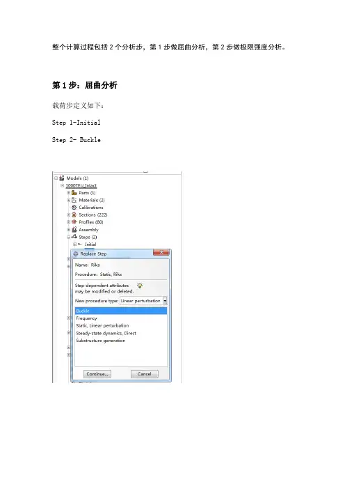
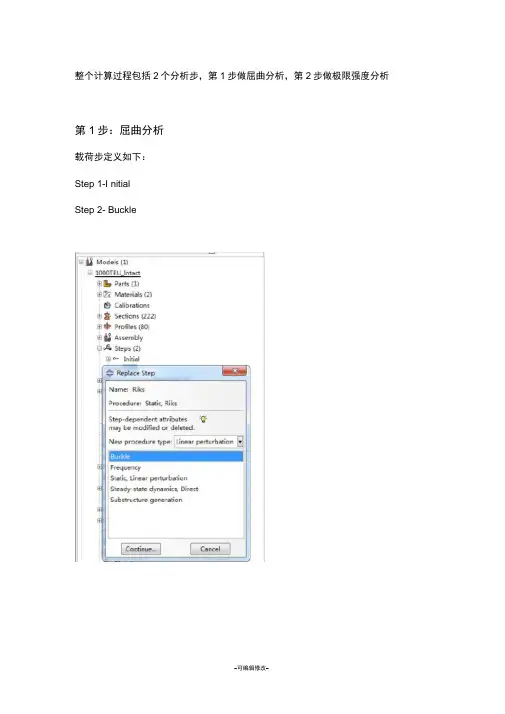
整个计算过程包括2个分析步，第1步做屈曲分析，第2步做极限强度分析。

第1步：屈曲分析载荷步定义如下：Step 1-InitialStep 2- Buckle并在Model-Edit Keywords的图中位置加入下面的文字，输出屈曲模态*nodefile, global=yesU,Create job 名称为“Buckling”点击continue，完成第1步的计算。

第2步：极限强度分析将“buckle”分析步替换为“riks”分析步在Basic选项卡中，Nlgeom：选择打开在Instrumentation选项卡中，定义如下参数，然后点击OK定义一个新计算工作，输入名称，点击continue在Parallelization选项卡，选择2个CPU，如下所示，点击OK。

在此编辑Model-edit keywords，删除“第1步”加入的文字“*nodefile, global=yesU,”，并在下图位置加入下段文字：*imperfection, file=buckling, step=11, 2.5点击OK，再保存文件。

最后提交计算。

提取计算结果进入visualization Module点击 Create XY data选择 ODB filed output，点击continuePosition选择 Unique Nodal， CF：point loads选择 CF2，再点击elements/nodes选项卡，选择跨中载荷加载点，最后点击save。

重复上一步操作，Position选择 Unique Nodal， U：spatial displacement 选择 U3，再点击elements/nodes选项卡，选择板格中心点，最后点击save。

点击Create XY data, 选择operate on XY data，点击continue选择Combine（X,X）命令，横坐标选择保存的displacement曲线，纵坐标选择保存的Point load曲线，点击最后一行Create XY Data与Save as。

ABAQUS非线性屈曲分析步骤分享：ABAQUS 非线性屈曲分析步骤来源：杨洋洋的日志riks法，或者general statics法（加阻尼），或者动力法一共三种方法，【问】在aba中能实现非线性屈曲分析吗？在step中选定line- perturbation下的各项，其Nlgeom都为Off，是不是意味着是进行不了啊？【答】line-perturbation应该是特征值屈曲分析，只能是线性的，要想进行非线性屈曲分析要引入初始缺陷ABAQUS中非线性屈曲分析采用riks算法实现，可以考虑材料非线性、几何非线性已经初始缺陷的影响。

其中，初始缺陷可以通过屈曲模态、振型以及一般节点位移来描述。

no.1: 利用abaqus进行屈曲分析，一般有两步，首先是特征值屈曲分析，此分析为线性屈曲分析，是在小变形的情况进行的，也即上面提到过的模态，目的是得出临界荷载（一般取一阶模态的eigenvalue乘以所设定的load），且需要在inp文件中，作如下修改*node file,global=yes*End Step此修改目的在于：在下一步后屈曲分析所需要的初始缺陷的节点输出为.fil文件。

no.2：其次，就是所谓的后屈曲分析，此步一般定义为非线性，原因在于是在大变形情况进行的，一般采用位移控制加修正的弧长法，可以定义材料非线性，以及几何非线性，加上初始确定，所以也称为非线性屈曲分析。

此步分析，为了得到极限值，需要得出荷载位移曲线的下降段，除了采用位移控制以及弧长法设定外，需在所得到的inp文件中，嵌入no.1中的.fil节点数据。

修改如下：*IMPERFECTION（缺陷）, FILE=results_file（此文件名为.fil）, STEP=step(特征值分析步名),1（模态），2e-3（模态的比例因子，此值一般取杆件的1%，壳体厚度1%）此修改一般加在boundary之后step之前。

Re:新手请教非线性屈曲中如何加初始扰动？6.2.4 Unstable collapse and postbuckling analysisRik法用于跳越失稳问题的研究，也可以用于分支屈曲的后屈曲研究。

整个计算过程包括2个分析步，第1步做屈曲分析，第2步做极限强度分析第1步：屈曲分析载荷步定义如下：Step 1-I nitialStep 2- Buckle]" BldMll% "Gfi hSM "Btifr女问g RM ：L44Lai4Jlb L-l-SteJ SW34 to*- &mp»hjiv9匂Pl DjeMfi.c-5 ba^a bm "一 ~Z te -!^l -Si|| v*V* IA4W f*i <pd貝呎■吟1 和訐ym 印炖d FMffv 讹V 匚曲反..76^* + r 、：：和A£T 巴：T=肛八FT •-百只“二o 土- .丫E案H IB ndi 4'B-rtBPCT14 FBW5^/W r«vfFK 口[• J甲■g CiM#»i4n M»oh totiG A g w^rirj出戶ii >W1MW4 >W#iTl4ChW曲比£丹71 怕iKSdUK«rtrin 导>F1MBB5M/WU ■T-**n *li«r I ll^hfli wThe jaj^.4toe 1 iibQL>j4| .h-2 內贞 J^r 11411 X>v m 均Lbit S KJ -1 Silled 3 EBri? pLufiE -汕 4 耳 D I si 泊■« 0TOD l&sm iy*i»Je !i?d bv 呵 ■怙O . -Ifcu 町临 Xrtpftii r* ihe 自他迈灯 曲妣仙哙 白jrttE The- K ^±L isi-SDfrse- :hs 当 be«i ami ID 'J T^*p AZLQIL L ISLCA :-se- 1 TT*s "4TAI1" Ikhli ^f4l ：h-9 W IVAntJiB'^fl ■帀 *4111 h I 10 1 iw*AW^ihl f iwwl I riAFe -4B4B-A* 并在 Model-Edit Keywords*no defile, global=yesU,聞 孕 ”询詡 fit 审 0(*r T*$l< Ruy-hi 孑母 ¥*口占■❷建It 十亡叫乐口輯1 •占0 lb S3'Void««dm« : 9 弱 »W M I .CL I .yariUi b **TI 插 ■ FA VW MT * 心■l* 町 E 岂 Std* g .Flibi■ y g 村啤. J "oft Ia* It 迅Qg I 宝 H ET I UTT Uid^ut t3 *W *«iTfc- 弘 4f Mu»Fr ] n ★”■■也… 册 feMvidrttar M fLcmtad 诵 CcmdllMMik Id C-uffin.1! 9 Mid lx （■miitov'h 'ZfftHeur bet 卜 J £«4* rt. ■— -■-,N^nd. —$ 1 ■曹 e R 1 °IfMK nev *w 居 The Ji-^.4hje ] UDQL3-J4I .n-J 沖女 j'lir alCil J>v 切 xbc^- atjft glic 讯 试 Ebt* pCy fili TQ . . I xiid "d 耳Or Q -iOD Ififi in-u w UitiJfl sd K 说 TBP .亠I 汕 «l!fa frSMcj C* llw 冃论迈叩 xcmLDi 哙 nwi««tr ：4=-L ftss t«e& xF w □ T -**p Ai&^ZL L IMA :-seii j * ■ih * i>¥ii "i4i ii -I -t>A4 TYE 巾尼‘旳！ B 帀 *rn n ■：riF YW «T in ib* 钻巒■nlM ・ e 1力『円「0，何■比 I 4- IJ I ■ Ml 曲 |Tfl4 hr r- fckdiie 4wne- M?p-]J 2加 甘植小乜CL fa W 31 E El KUhF* !1, 审 WlitM '■ g ^Ktd -IHC EIl ⑷册冇 Qg K aii e/y - B A ‘ 宝Hwlwr U I J^U ! t3 W-^SM B -in «U 4rrt^Ta* %n I H H wli aE 甘 hltnarl 旨內岭A] H CjMivi CdMT9 if C-OHKlInMt ： 昭 I Mali创（-miitoMilj■ Ejwrfnr fact .f Mb乞H B 『鼻為& -x J r T n 一 ：w 0 MoM fMhW-L ■灰 OM4L LE 中鼻Eai OfMW rti p T !--^ IdHI f - A ・■*<< X ・（V ）屮 d 1*",・L=> ":昭!：站我 tbrian I ；E ■毗 CH-^R W«W^r. r<jw|a<r or ■ftoritf flvfFML LMII ^ sewihiH ・ ・H rr*Mi «<h rapd TK I M ar 4-cai p^ak^ad ■3=n> #ia ari -jn^tDr cad Ktk wrii:・ Mid… . PF T4J P «■ c * ® '■ ■ 29WW^ n.^.的图中位置加入下面的文字，输出屈曲模态Create job 名称为“ Buckling点击continue ，完成第1步的计算(D &eJfiew Sfte 口 Output Other loo-S Mug-in? Q ［予 &J*nager..s & ModflL| Copy Modd 卜宕htod 亡呻O^Kt —\二也・ 甘 L宀 Ed4 Anri butts • Modd Viewport: 匕匕口人t 2 3 4 Modu *t 「-： Modd ： x Rf^inw ► L 占 | Q slrt 电 . C> C^al ibralsDFS 4 S' Sectior-g (2221 _. -ix n __ i —. tafn第2步：极限强度分析将“ buckle ”分析步替换为“ riks ”分析步”二AE - -4J 1Bk 歴詔#1 嶠如pxt 垦w Qwpv* Other £M I*H呼戸屮L MRk +<* %女X M iM UnPnUdA 1®I {jiad— Vipjrptitl 乩疏1IF Jib-lpji Othgr Icids. s ij^'ns. £j?lp 审I J3S-中C叫匚却u g M 1Morit Re^yiii舜I制讶甘：QI |2 Meddf (I)::誠贰右ParH Q|jf |?< Mawfiaic i；7)宫Giibr』口M菟Sr Swtbn, [223fc> ZT I8UIbupt lilF*=，Qi Pi"； i； HiE 伍*M«teriali [2| fir tiEH-i.蛊h«Bor-s J_ - I 幸Pr^le i (KB■出Al i^ltlLiji 咼bbt印L -S Hitch Conlcxl Orl t S^piHeM B*»C C-iPTEr-*Time PALE AdMlJirftrratIwac Elm. &Hlfomtc iHipp^rtifi*Cc^ldc s■Cmitr;AddsAmoIrtLLo^di <^7W Ai HmEEiDMd &l Urd-rCall^pse JLJI LlndtrAridOHisscryModUt r 趾P■心ESIM CK：U I« rSlep在Basic 选项卡中，Nlgeom :选择打开在Instrumentation 选项卡中，定义如下参数，然后点击 Oih«rTI «•4^-rarpJlk ■ P -.uadlumbar & hcd«fn»rM ：Iniiid Mnmurn MagnumArc le-^ih rKmiwc C J OI. L£-D15 ilfOJdE^mjied nzcdJ 1Ncrtt: Used] off tu rcompute :he DA lobd pruRiHiorin ry 口書定义一个新计算工作，输入名称，点击 con ti nueOK N JIE ■: Rika。

压杆屈曲分析1.问题描述在钢结构中，受压杆件一般在其达到极限承载力前就会丧失稳定性，所以失稳是钢结构最为突出的问题。

压杆整体失稳形式可以是弯曲、扭转和弯扭。

钢构件在轴心压力作用下，弯曲失稳是常见的失稳形式。

影响轴心受压构件整体稳定性的主要因素为纵向残余应力、初始弯曲、荷载初偏心及端部约束条件等。

实际的轴心受压构件往往会存在上述的一种或多种缺陷，导致构件的稳定承载力降低。

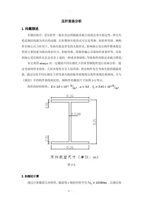
本文利用abaqus 对一定截面不同长细比下的H 型钢构件进行屈曲分析，通过考虑材料非线性、几何非线性并引入初弯曲，得出构件发生弯曲失稳的极限荷载。

通过比较不同长细比下的弯曲失稳的临界荷载得出构件荷载位移曲线，并与《规范》中的构件曲线相比较。

钢构件的截面尺寸如图1-1所示。

构件的材料特性： E =2.0×1011 N m 2⁄ ,μ=0.3 , f y =3.45×108N m 2⁄图1-12.长细比计算 通过计算截面几何特性，截面绕y 轴的回转半径为i y =0.0384m ,长细比取压杆截面尺寸（单位：m）值及杆件长度见表1：表13.模型分析ABAQUS非线性屈曲分析的方法有riks法，general statics法（加阻尼），或者动力法。

非线性屈曲分析采用riks算法实现，可以考虑材料非线性、几何非线性已及初始缺陷的影响。

其中，初始缺陷可以通过屈曲模态、振型以及一般节点位移来描述。

利用abaqus进行屈曲分析，一般有两步，首先是特征值屈曲分析，此分析为线性屈曲分析，是在小变形的情况进行的，也即上面提到过的模态，目的是得出临界荷载（一般取一阶模态的eigenvalue乘以所设定的load）。

其次，就是后屈曲分析，此步一般定义为非线性，原因在于是在大变形情况进行的，一般采用位移控制加修正的弧长法，可以定义材料非线性，以及几何非线性，加上初始缺陷，所以也称为非线性屈曲分析。

此步分析，为了得到极限值，需要得出荷载位移曲线的下降段。

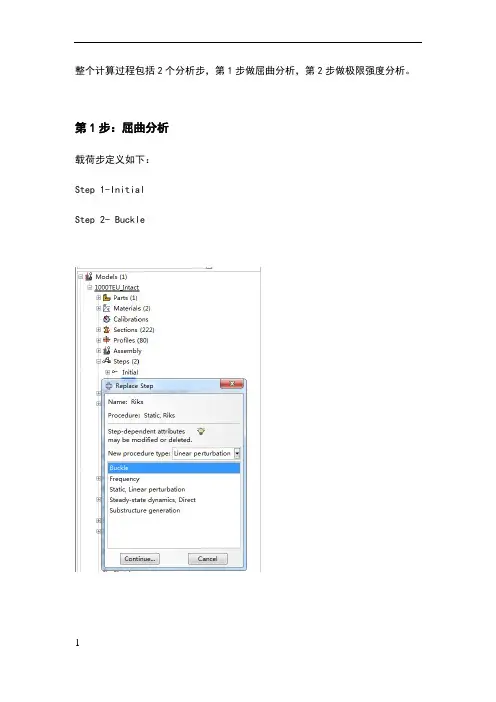
整个计算过程包括2个分析步，第1步做屈曲分析，第2步做极限强度分析。

第1步：屈曲分析载荷步定义如下：Step 1-InitialStep 2- Buckle并在Model-Edit Keywords的图中位置加入下面的文字，输出屈曲模态*nodefile, global=yesU,Create job 名称为“Buckling”点击continue，完成第1步的计算。

第2步：极限强度分析将“buckle”分析步替换为“riks”分析步在Basic选项卡中，Nlgeom：选择打开在Instrumentation选项卡中，定义如下参数，然后点击OK定义一个新计算工作，输入名称，点击continue在Parallelization选项卡，选择2个CPU，如下所示，点击OK。

在此编辑Model-edit keywords，删除“第1步”加入的文字“*nodefile, global=yesU,”，并在下图位置加入下段文字：*imperfection, file=buckling, step=11,点击OK，再保存文件。

最后提交计算。

提取计算结果进入visualization Module 点击 Create XY data选择 ODB filed output，点击continuePosition选择 Unique Nodal， CF：point loads选择 CF2，再点击elements/nodes选项卡，选择跨中载荷加载点，最后点击save。

重复上一步操作，Position选择 Unique Nodal， U：spatial displacement 选择 U3，再点击elements/nodes选项卡，选择板格中心点，最后点击save。

点击Create XY data, 选择operate on XY data，点击continue选择Combine（X,X）命令，横坐标选择保存的displacement曲线，纵坐标选择保存的Point load曲线，点击最后一行Create XY Data与Save as。