zemax_优化函数说明书
- 格式:pdf
- 大小:415.65 KB
- 文档页数:23

优化函数1、像差SPHA(球差):surf表面编号/wave波长/target设定目标值/weight权重指定表面产生的球差贡献值,以波长表示。
如果表面编号值为零,则为整个系统的总和COMA(彗差) :surf表面编号/wave波长/target设定目标值/weight权重指定表面产生的贡献值,以波长表示。
如果表面编号值为0,则是针对整个系统。
这是由塞得和数计算得到的第三级彗差,对非近轴系统无效.ASTI(像散):指定表面产生像散的贡献值,以波长表示。
如果表面编号值为0,则是针对整个系统。
这是由塞得和数计算得到的第三级色散,对非近轴系统无效FCUR(场曲):指定表面产生的场曲贡献值,以波长表示。
如果表面编号值为0,则是计算整个系统的场曲。
这是由塞得系数计算出的第三级场曲,对非近轴系统无效.DIST(畸变):指定表面产生的畸变贡献值,以波长表示。
如果表面编号值为0,则使用整个系统。
同样,如果表面编号值为0,则畸变以百分数形式给出。
这是由塞得系数计算出的第三级畸变,对与非近轴系统无效.DIMX(最大畸变值):它与DIST 相似,只不过它仅规定了畸变的绝对值的上限。
视场的整数编号可以是0,这说明使用最大的视场坐标,也可以是任何有效的视场编号。
注意,最大的畸变不一定总是在最大视场处产生。
得到的值总是以百分数为单位,以系统作为一个整体。
这个操作数对于非旋转对称系统可能无效。
AXCL(轴向色差):以镜头长度单位为单位的轴向色差。
这是两种定义的最边缘的波长的理想焦面的间隔。
这个距离是沿着Z 轴测量的。
对非近轴系统无效.LACL(垂轴色差):这是定义的两种极端波长的主光线截点的y方向的距离。
对于非近轴系统无效TRAR(垂轴像差):在像面半径方向测定的相对于主光线的垂轴像差.TRAX(x方向垂轴像差):在像面x方向测定的相对于主光线的垂轴像差TRAY(Y方向垂轴像差):在像面Y方向测定的相对于主光线的垂轴像差TRAI(垂轴像差):在指定表面半口径方向测定的相对于主光线的垂轴像差.类似于TRAR,只不过是针对一个表面,而不是指定的像面.OPDC(光程差):指定波长的主光线的光程差.PETZ(匹兹伐曲率半径):以镜头长度单位表示,对非近轴系统无效PETC(匹兹伐曲率):以镜头长度单位的倒数表示,对非近轴系统无效RSCH:相对于主光线的RMS 斑点尺寸(光线像差)。
zemax主要优化函数(ZEMAX main optimization function)ZEMAX main optimization function table, 2008 28 Monday 07 00:53 optimization functionAberration 1SPHA (spherical aberration):surf surface number /wave, wavelength /target, set target value, /weight weightThe contribution of the spherical aberration to the specified surface is represented by wavelengths. If the surface number is zero, it is the sum of the entire systemCOMA (coma):surf surface number /wave wavelength /target target value /weight weightSpecify the contribution value of the surface, expressed in wavelength. If the surface number is 0, it is for the entire system. This isAnd as calculated by the number of third level coma of non paraxial invalid system.ASTI (astigmatism): Specifies the contribution of a surface to astigmatism, represented by wavelengths. If the surface number is 0, it is for the entire system. This is the third level was calculated by dispersion and number of non paraxial, invalid systemFCUR (field curvature): specify the contribution of the surface to the field, expressed at wavelengths. If the surface numberis 0, then the whole system is calculated. This is the third level was calculated by the field curvature coefficient, the non paraxial invalid system.DIST (distortion): Specifies the contribution of a surface to distortion, expressed as a wavelength. If the surface number is 0, the entire system is used. Similarly, if the surface number is 0, the distortion is given in percentage. This is the third level was calculated by the distortion coefficient of non paraxial, and invalid system.DIMX (maximum distortion): it is similar to DIST, but it only specifies the upper limit of the absolute value of distortion. The integer number of the field of view can be 0, indicating the use of the maximum field of view coordinates, or any valid field number. Note that the greatest distortion does not always occur at the maximum field of view. The resulting value is always in percentage, and the system as a whole. This operand may be invalid for a non rotationally symmetric system.AXCL (axial chromatic aberration): axial chromatic aberration in units of lens length. This is the two definition of the most marginal wavelength of the ideal focal plane interval. This distance is measured along the Z axis. Is not valid for non paraxial systemsLACL (vertical axis chromatic aberration): This is the distance of the Y direction of the main light point of the two extreme wavelengths defined. Invalid for non paraxial systemsTRAR (vertical axis aberrations): vertical aberrationsrelative to the main light measured in the direction of the image plane radiusTRAX (x direction vertical axis aberrations): vertical aberrations relative to the main light measured in the image plane xTRAY (Y direction vertical axis aberrations): vertical aberrations relative to the main light measured in the image plane YTRAI (vertical axis aberration): vertical aberrations in the specified surface half aperture direction relative to the main light. Similar to TRAR, only for a surface, not for a specified image planeOPDC (Guang Chengcha): the optical path difference of the primary ray of the specified wavelengthPETZ (Petzval curvature radius): the length of the lens unit, non paraxial system of invalidPETC (Petzval curvature): the reciprocal of length of the lens unit, the non paraxial invalid systemRSCH: the RMS spot size (light aberration) relative to the main light.RSCE: Hx, Hy, measured by the length of a lens, relative to the geometric centroid of the RMS spot (ray aberration).This operand is similar to RSCH, except that the reference point is like the centroid, not the primary ray. For details, see RSCH. R0Y}N ~Q!The RWCH: band wavelength Hx, Hy, is relative to the RMS wavefront difference of the main light. Its unit is wavelength. Since the average OPD has been subtracted, this RMS actually refers to the standard wavefront deviation. See RWCE. For details, see RSCHBRWCE: the band gap Hx, Hy, and the RMS wavefront difference relative to the diffraction centroid. This operation is useful for minimizing the wavefront deviation, deviation from the wavefront Strehl ratio and the MTF area under the curve is proportional to the. Its unit is wavelength. See RWCH. For details, see RSCHANAR: the angle difference radius of the main light relative to the main wavelength measured on an image plane. This number is defined as 1-cos theta theta, here is between the traced rays and the angle of the light. See TRARZERN: Zernike edge factor. The coefficient terms Int1, Int2, Hx, and Hy data values are used to specify the number of Zernike coefficient terms (1-37), the wavelength number, the sampling density (1=32*32, 2=64*64, etc.) and the field of view position. Note that if you have multiple ZERN operands with only variable number of entries, they should be placed in adjacent rows at the edit interface. Otherwise, the computation speed will be reducedTRAC: vertical axis aberrations relative to the center of mass in the direction of the image plane radius. Unlike other operands, TRAC works correctly according to the distribution of other TRAC operands in the edit function of the evaluation function. TRAC operands must be grouped together by field of view and wavelength. ZEMAX will trace all the TRAC rays of a common field of view together, and then calculate the centroid of all the light based on these collective data. Only the default evaluation function tool is used to import this operand into the evaluation function editing interface, rather than advising the user to use it directly.OPDX: this sphere can minimize the RMS wavefront difference relative to the optical path difference of a moving and tilted sphere; here, ZEMAX uses the centroid reference. OPDX has the same constraints as TRAC. See TRAC for more details.RSRE: grid wavelength Hx, Hy, measured by the length of a lens unit, relative to the geometric centroid of the RMS dot size (ray aberration). This operand is similar to RSCE, except that it uses the light of the rectangular mesh rather than the Gauss integral method. This operand is generally accepted for vignetting. A grid value of 1 represents 4 rays, 2 represents a trace, each quadrant tracks a 2*2 mesh (16 rays), and 3 represents a 3*3 grid (36 rays) per quadrant, and so on. The symmetry of the system has been taken into accountRSRH: similar to RSRE, but the reference point is the main light.RWRH: similar to RSRH, it's only calculating wavefrontdifferences, not speckle sizesRWRE: similar to RSRE, it's only calculating wavefront differences, not speckle sizes.The x component of TRAD:TRAR. TRAD has the same constraints as TRAC. See TRAC for more details.The Y component of TRAE:TRAR. TRAD has the same constraints as TRAC. See TRAC for more detailsX: vertical aberrations relative to the center of mass measured in the direction of the image plane TRCX.See TRAC. Only the default evaluation function tool is used to import this operand into the evaluation function editing interface, rather than advising the user to use it directly.Y: vertical aberrations relative to the center of mass measured in the direction of the image plane TRCYDISG: generalized distortion, the reference field wavelength is. Expressed as a percentage. This operator calculates the distortion of any light at any wavelength and in any field of view, taking any field of view as a reference. The method of use and the assumptions you make are the same as those described in the chapter on the analysis menuFCGS: normalized sagittal field curvature. The field values are calculated for each wavelength, each field of view. Normalization of this value yields a reasonable result, evenfor non rotationally symmetric systems. See the analysis of the field features in the menu Chapter 32 "1 & S"FCGT: normalized meridional field curve.DISC: normalized distortion. This operand calculates the normalized distortion of the entire visible field, and obtains the absolute value of the maximum non-linear value for the f- theta condition. This operand is very useful for the design of those f- theta lenses. -Y 0uB;OPDM: the optical path difference relative to the average OPD; this operand is calculated from the average OPD of all rays on the pupil as a reference to the OPD value. OPDM has the same constraints as TRAC. See TRACn BZ=Ytl A for more detailsBSER: Aiming error. Semi coordinates are divided by the effective focal length is defined as the main light aiming error traced on the field axis. This definition will produce measurements of the angular deviation of the image. A`mP-MKTp'Id9C'+^]2, modulation letter xDTy 7$KZD@FpGL 8, XqMTFT: the square wave modulation transfer function value of meridian. Sampling density wavelength. It calculates the diffraction MTF value. The parameter Int1 must be an integer (1, 2, 3)... ) 1 produces a sampling density of 32*32, 2 producesa sampling density of 64*64, and so forth. The Int2 must be a valid wavelength number, or 0, representing all wavelengths. The value of Hx must be a valid field number (1, 2)... .). Hy is the spatial frequency expressed in cycles per millimeter. If the computational accuracy of the sampling density relative to MTF is too low, all operands MTF will get zero values. If both meridian and sagittal MTF are required, they are placed in adjacent rows, MTFT and MTFS, which are computed simultaneously. See the instructions for the use of operand MTF in this chapter in more detail. P.BD4 T $MTFS: the modulation transfer function value of the arc vector. For details, see "MTFT"". F, G, l, jMTFA: the mean value of the modulation transfer function of the arc vector and the meridian. For details, see "MTFT"". |'p dg!MSWT: the square wave modulation transfer function value of meridian. For details, see "MTFT"". &Lt{p l8u6MSWS: the square wave modulation transfer function value of the arc vector. V4W0 shall 6MSWA: the mean square of the square wave modulation transfer function of the sagittal and meridional. For details, see "MTFT"". \`cp=OY[ZGMTA: the geometric transfer function of arc vector and meridian, the mean of response curve. The parameter Int1 must be an integer (1, 2,...) 1 produce 32*32 sampling density, 2 produce 64*64 sampling density, and so on.Int2 can be any valid wavelength number, or 0, representing all wavelengths. The value of Hx must be a valid field number (1, 2,...). Hy is the spatial frequency expressed in cycles per millimeter. Px is a marker, and if it is 0, the diffraction limit is used to scale the transfer function values (recommended), otherwise they are not scaled. See the section on the use of operand MTF in this chapter for more details. O$zn+5f9/GMTS: the geometric transfer function response curve of the arrow vector. See the operands GMTA., I, SDlS, G in detailGMTT: Meridian geometric transfer function response curve, in detail, see operand GMTA.WbP, Bp{| Gy =< Y3. Basic optical properties /X2, A, uU (#]. /EFFL: the effective focal length is expressed in units of lens length. It is aimed at the paraxial system, and for non paraxial systems may be inaccurate U:o`/4 "XL"PIMH: the image height on the paraxial image plane of the specified wavelength. A@+3- 0/PMAG: paraxial magnification. This is the ratio of the height of the paraxial main light to the height of the paraxial image plane. Only useful for finite far conjugate systems. Note thatthe near axis image plane can be used even though the system cannot be ideal focused. T w% CwCR5AMAG: angle magnification. This is the ratio of the angle of the main axis of the light between the space and the object space. For non paraxial systems, invalid 3, l, {DE \ENPP: relative to the first surface, the pupil position is indicated by the unit of lens length. This is the paraxial pupil position, valid only for the central system, 9 nG MEXPP: expressed as a unit of lens length relative to the pupil position of the first face. This is the paraxial pupil position, valid only for the central system, A>, Ktl, uLINV: the Lagrange invariants of a system, expressed in units of lens length. Calculate the value MJ 8 & s=y with the paraxial edge light and the main ray dataWFNO: work, F/#. This is calculated from the angle of the actual edge light in the space relative to the main light. SN e E; KPOWR: the weight of the specified number of surfaces (represented by reciprocal units of the length of the lens). This operand is only valid for standard surfaces. Surface numbering &HI^ \ =EPDI: the pupil diameter is expressed in units of lens length. P 85ISFN: like space, F/#. This operand is infinite and conjugatenear axis F/#. See "WFNO" D, bP\}#aEFLX: the effective focal length of the primary wavelength of the surface in the specified range on the fixed X plane is expressed in terms of the length of the lens. The number of the first surface and the number of the last surface. */x9_Lo ^EFLY: the effective focal length of the main wavelength of the surface in the specified range on the fixed Y plane. The jCg <L is expressed in terms of the length of the lens;SFNO: the sagittal work F/# calculated at any defined field of view and wavelength. See TFNO. The field of view is S -F|5 "Sp"TFNO: the meridional work F/# calculated at any defined field of view and wavelength. See SFNO. WN\ sfnJURIMAG: image resolution. No matter what the default settings are currently used, this operand has the same resolution as the result of the geometric image analysis. To use this operand, you must first define the set values in the geometry analysis feature,Then press the Save button in the settings box. The operand IMAE will have the same resolution (normalization) as the image analysis feature. See the instructions in the optimization of the operand IMAE below.。


优化函数1、像差SPHA(球差):surf表面编号/wave波长/target设定目标值/weight权重指定表面产生的球差贡献值,以波长表示。
如果表面编号值为零,则为整个系统的总和COMA(彗差) :surf表面编号/wave波长/target设定目标值/weight权重指定表面产生的贡献值,以波长表示。
如果表面编号值为0,则是针对整个系统。
这是由塞得和数计算得到的第三级彗差,对非近轴系统无效.ASTI(像散):指定表面产生像散的贡献值,以波长表示。
如果表面编号值为0,则是针对整个系统。
这是由塞得和数计算得到的第三级色散,对非近轴系统无效FCUR(场曲):指定表面产生的场曲贡献值,以波长表示。
如果表面编号值为0,则是计算整个系统的场曲。
这是由塞得系数计算出的第三级场曲,对非近轴系统无效.DIST(畸变):指定表面产生的畸变贡献值,以波长表示。
如果表面编号值为0,则使用整个系统。
同样,如果表面编号值为0,则畸变以百分数形式给出。
这是由塞得系数计算出的第三级畸变,对与非近轴系统无效.DIMX(最大畸变值):它与DIST 相似,只不过它仅规定了畸变的绝对值的上限。
视场的整数编号可以是0,这说明使用最大的视场坐标,也可以是任何有效的视场编号。
注意,最大的畸变不一定总是在最大视场处产生。
得到的值总是以百分数为单位,以系统作为一个整体。
这个操作数对于非旋转对称系统可能无效。
AXCL(轴向色差):以镜头长度单位为单位的轴向色差。
这是两种定义的最边缘的波长的理想焦面的间隔。
这个距离是沿着Z 轴测量的。
对非近轴系统无效.LACL(垂轴色差):这是定义的两种极端波长的主光线截点的y方向的距离。
对于非近轴系统无效TRAR(垂轴像差):在像面半径方向测定的相对于主光线的垂轴像差.TRAX(x方向垂轴像差):在像面x方向测定的相对于主光线的垂轴像差TRAY(Y方向垂轴像差):在像面Y方向测定的相对于主光线的垂轴像差TRAI(垂轴像差):在指定表面半口径方向测定的相对于主光线的垂轴像差.类似于TRAR,只不过是针对一个表面,而不是指定的像面.OPDC(光程差):指定波长的主光线的光程差.PETZ(匹兹伐曲率半径):以镜头长度单位表示,对非近轴系统无效PETC(匹兹伐曲率):以镜头长度单位的倒数表示,对非近轴系统无效RSCH:相对于主光线的RMS 斑点尺寸(光线像差)。


zemax优化函数使用方法Zemax是一款常用于光学系统设计和优化的软件工具。
其中的优化函数是Zemax的一个重要功能,可以帮助用户通过自动搜索和调整系统参数,找到最优的设计方案。
本文将介绍Zemax优化函数的使用方法。
一、什么是优化函数在光学系统设计中,我们通常需要通过调整系统的各种参数来实现特定的设计要求。
而优化函数就是帮助我们在众多参数中找到最优解的工具。
其原理是通过数值计算和模拟,自动化地搜索参数空间,以寻找最佳的设计方案。
二、Zemax中的优化函数Zemax中的优化函数可以分为两大类:单变量优化和多变量优化。
单变量优化是指只有一个参数需要进行调整,而多变量优化则是同时调整多个参数。
下面将分别介绍这两种优化函数的使用方法。
1. 单变量优化函数单变量优化函数可以通过调整一个参数,来寻找最优解。
在Zemax 中,我们可以选择需要调整的参数,并设置其变化的范围和步长。
然后,通过运行优化函数,Zemax会自动搜索参数空间,并给出最优的结果。
2. 多变量优化函数多变量优化函数可以同时调整多个参数,以找到最优解。
在Zemax 中,我们可以选择多个参数,并设置它们的变化范围。
然后,通过运行优化函数,Zemax会自动搜索多个参数的组合,并给出最佳的设计方案。
三、使用优化函数的步骤使用Zemax的优化函数,一般需要按照以下步骤进行操作:1. 定义优化目标:首先,我们需要明确设计的目标和要求,例如最小化像差、最大化光学传输等。
这样才能设置正确的优化函数和参数。
2. 设置参数范围:根据设计要求,我们需要选择需要调整的参数,并设置它们的变化范围。
例如,镜片的曲率半径、透镜的厚度等。
3. 运行优化函数:在Zemax中,我们可以选择不同的优化函数进行计算。
例如,全局优化、局部优化等。
根据设计要求和参数设置,选择适合的优化函数,并运行它。
4. 分析结果:运行完优化函数后,Zemax会给出最优的设计方案。
我们可以通过分析结果,评估设计的优劣,并进行进一步的优化和改进。

zemax主要优化函数zemax主要优化函数表2008年07月28日星期一 00:53优化函数1、像差SPHA(球差):surf表面编号/wave波长/target设定目标值/weight权重指定表面产生的球差贡献值,以波长表示。
如果表面编号值为零,则为整个系统的总和COMA(彗差) :surf表面编号/wave波长/target设定目标值/weight权重指定表面产生的贡献值,以波长表示。
如果表面编号值为 0,则是针对整个系统。
这是由塞得和数计算得到的第三级彗差,对非近轴系统无效.ASTI(像散):指定表面产生像散的贡献值,以波长表示。
如果表面编号值为0,则是针对整个系统。
这是由塞得和数计算得到的第三级色散,对非近轴系统无效 FCUR(场曲):指定表面产生的场曲贡献值,以波长表示。
如果表面编号值为0,则是计算整个系统的场曲。
这是由塞得系数计算出的第三级场曲,对非近轴系统无效.DIST(畸变):指定表面产生的畸变贡献值,以波长表示。
如果表面编号值为0,则使用整个系统。
同样,如果表面编号值为 0,则畸变以百分数形式给出。
这是由塞得系数计算出的第三级畸变,对与非近轴系统无效.DIMX(最大畸变值):它与 DIST 相似,只不过它仅规定了畸变的绝对值的上限。
视场的整数编号可以是 0,这说明使用最大的视场坐标,也可以是任何有效的视场编号。
注意,最大的畸变不一定总是在最大视场处产生。
得到的值总是以百分数为单位,以系统作为一个整体。
这个操作数对于非旋转对称系统可能无效。
AXCL(轴向色差):以镜头长度单位为单位的轴向色差。
这是两种定义的最边缘的波长的理想焦面的间隔。
这个距离是沿着Z 轴测量的。
对非近轴系统无效. LACL(垂轴色差):这是定义的两种极端波长的主光线截点的y方向的距离。
对于非近轴系统无效TRAR(垂轴像差):在像面半径方向测定的相对于主光线的垂轴像差. TRAX(x方向垂轴像差):在像面x方向测定的相对于主光线的垂轴像差 TRAY(Y方向垂轴像差):在像面Y方向测定的相对于主光线的垂轴像差 TRAI(垂轴像差):在指定表面半口径方向测定的相对于主光线的垂轴像差.类似于 TRAR,只不过是针对一个表面,而不是指定的像面.OPDC(光程差):指定波长的主光线的光程差.PETZ(匹兹伐曲率半径):以镜头长度单位表示,对非近轴系统无效 PETC(匹兹伐曲率):以镜头长度单位的倒数表示,对非近轴系统无效 RSCH:相对于主光线的RMS 斑点尺寸(光线像差)。
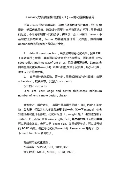
Zemax-光学系统设计经验(1)---优化函数的使用使用Zemax设计光学系统,基本上就是根据设计要求,给出初始设计,然后优化系统。
初始设计需要对光学有系统的学习,需要长期的经验,不同的领域有不同的要求,初始设计会大不相同,zemax不会给你太多的帮助。
Zemax的精髓是能计算出光路图,然后使用operand(优化函数)优化各项光学参数。
1. default merit function,当属最有用的优化函数,配合EFFL (有效焦距)使用,基本可以设计大部分光学系统。
可以使用RMS spot radius and rms wavefront error。
另外设置好变量。
Zemax会自动生成优化系数(weight). 函数行的量取决于波长数,场(field)数,也决定了计算的快慢。
2. 自己设计优化函数。
第一步,需要知道你的优化目标:焦距,abberation,耦合效率。
设置好constraints.设计的constraints:Lens size, cost; edge and center thickeness; minimum number of lens; simple design; cheap举例来讲,耦合效率。
有两个最有用的函数:FICL, POPD. 前者快,后者慢,但后者对大多数系统要准确一些。
读一下manual,你会知道你要设置什么参数。
优化目标是1,weight 是1. 要知道在哪个surface上,还有在什么wavelength, field, 最重要的是什么优化数据,可以是耦合效率,也可以是beam size。
如果都要考虑,可以设置新的POPD函数,设置好优化系数(weight). 有例子,改一下merit function就可以了。
有些有用的优化函数:加减乘除:SUMM, DIFF, PROD,DIVI镜头数据:MXCG, MNCG, CTGT, MNCT,变量的设置也很有讲究,越多越靠近理想目标,但是降低速度和提高坏设计的几率.几点经验:1. 尽可能 use solve, instead of 变量2. 尽可能 use default merit function3. 理解constraints4. 理解和使用symmetry5. 去掉无用的变量.6. 知道怎么去改变设计。
![zemax优化[资料]](https://uimg.taocdn.com/38efa4ebc9d376eeaeaad1f34693daef5ef713a1.webp)
(3).(4).(5).000双胶合透镜的初始结构参数为:000优化步骤:0001.在评价函数的操作数中输入有效焦距EFFL,目标值为43.33.权重为1.垂轴放大率PMAG,目标值为-0.5,权重为1.加入轴上点全孔径d光的纵向像差LONA,轴上点0.707孔径下F光和C光的轴向色差AXCL00和正弦差OSCD,目标值为0,权重为1.0002.把球差较大的2.3 面的曲率半径设为变量开始优化,然后再把1面的曲率半径也设为变量自动优化.000在评价函数的操作数中加上像距TOTR,目标值为65,权重为1. 自动优化,然后调整这个目标数,使优化达到最好,最后数为68.4.为了使初始结构的像距不至于改变太大,固定为64.由于厚度对优化不时很敏感,不把厚度作为变量,且由最小厚度选的值便于加工且成本最低.0 003.从pre中可以发现优化后的NA值只有0.098. 于是试着增大有效焦距的目标值,发现MTF曲线有所改善,最后在43.42处找到最好的优化点.004.为了更好的改善MTF的曲线,发现在频率126lp/mm处与衍射极限处相差最大.于是加入操作数子午的传递函数MTFT,目标值为0.5, 权重为1.最后优化得满足要求的曲线.000最后的评价函数操作数:000优化后的结构参数为:000优化后的MTF曲线(取主频率30 lp/mm):00优化后的二维结构图为: 共轭距为195.0000mm. 000优化后的点列图和各种像差曲线为:000优化后系统的像差(赛得和数)为:000双胶合透镜的二级光谱色差为:△l'= -f'(p1-p2)/(v1-v2)其中,p1,p2和v1,v2 分别为两种消色差材料的相对部分色散和阿贝数.000经查表可得:p1=0.01015. p2 =0.02431. v1=56.0. v2=29.5.000优化后的焦距为43.410513.000。
zemax主要优化函数表zemax主要优化函数表2009-11-17 15:05优化函数1、像差SPHA(球差):surf表面编号/wave波长/target设定目标值/weight权重指定表面产生的球差贡献值,以波长表示。
如果表面编号值为零,则为整个系统的总和COMA(彗差) :surf表面编号/wave波长/target设定目标值/weight权重指定表面产生的贡献值,以波长表示。
如果表面编号值为0,则是针对整个系统。
这是由塞得和数计算得到的第三级彗差,对非近轴系统无效. ASTI(像散):指定表面产生像散的贡献值,以波长表示。
如果表面编号值为0,则是针对整个系统。
这是由塞得和数计算得到的第三级色散,对非近轴系统无效FCUR(场曲):指定表面产生的场曲贡献值,以波长表示。
如果表面编号值为0,则是计算整个系统的场曲。
这是由塞得系数计算出的第三级场曲,对非近轴系统无效.DIST(畸变):指定表面产生的畸变贡献值,以波长表示。
如果表面编号值为0,则使用整个系统。
同样,如果表面编号值为0,则畸变以百分数形式给出。
这是由塞得系数计算出的第三级畸变,对与非近轴系统无效.DIMX(最大畸变值):它与DIST 相似,只不过它仅规定了畸变的绝对值的上限。
视场的整数编号可以是0,这说明使用最大的视场坐标,也可以是任何有效的视场编号。
注意,最大的畸变不一定总是在最大视场处产生。
得到的值总是以百分数为单位,以系统作为一个整体。
这个操作数对于非旋转对称系统可能无效。
AXCL(轴向色差):以镜头长度单位为单位的轴向色差。
这是两种定义的最边缘的波长的理想焦面的间隔。
这个距离是沿着Z 轴测量的。
对非近轴系统无效.LACL(垂轴色差):这是定义的两种极端波长的主光线截点的y方向的距离。
对于非近轴系统无效TRAR(垂轴像差):在像面半径方向测定的相对于主光线的垂轴像差.TRAX(x方向垂轴像差):在像面x方向测定的相对于主光线的垂轴像差TRAY(Y方向垂轴像差):在像面Y方向测定的相对于主光线的垂轴像差TRAI(垂轴像差):在指定表面半口径方向测定的相对于主光线的垂轴像差.类似于TRAR,只不过是针对一个表面,而不是指定的像面.OPDC(光程差):指定波长的主光线的光程差.PETZ(匹兹伐曲率半径):以镜头长度单位表示,对非近轴系统无效PETC(匹兹伐曲率):以镜头长度单位的倒数表示,对非近轴系统无效RSCH:相对于主光线的RMS 斑点尺寸(光线像差)。
ZEMAX操作说明一、参数设置1、透镜基本参数设置①、Surf:Type这一选项表示输入面的类型,例如普通球面、柱面、镜面、渐变折射率面等。
②、Comment这一选项表示对输入面进行注解,填不填都可以。
③、Radius这一选项表示输入面的曲率半径,对于第一行输入光源来说如果是Infinity表示光源为平行光,如果输入数字a表示距离透镜第一个面距离为a的点光源。
④、Thickness这一选项表示输入相邻两个面的距离,对于一个透镜来说是透镜的中心厚度,对于两个透镜来说是两个透镜的间距。
⑤、Glass这一选项表示输入相邻两个面间的材质,可以输入玻璃、镜子、接收器,不输为空气。
⑥、Semi-Diameter这一选项表示输入光到达通光面的半径。
⑦、Conic这一选项表示输入面曲率半径的非球面系数。
2、光源基本参数设置①、GenEntrance Pupil Diameter表示入射光到达第一个面时的光斑大小,适用于光源为点光源或平行光。
Object Space NA表示入射光的数值孔径,适用于点光源。
②、Fie这一选项表示对输入光在入射面不同输入高度时的情况。
③、Wav这一选项表示对输入光的波长。
④、Lay和L3d这一选项表示输入透镜的平面图和3D图⑤、Spt这一选项表示输入光通过输入透镜后的弥散斑的大小,越小越好。
⑥、Mtf这一选项表示输入透镜的传递函数,与分辨率紧密相关。
⑦、Pre这一选项表示输入透镜的所有参数汇总表。
二、设计结果查看在Analysis一项中查看透镜像差。
初步学习在这一项中一般查看:Image Analysis,这一项中可以直观查看成像质量。
Miscellaneous,这一项中可以查看输入透镜的像差。
三、透镜优化1、双击你所需要优化的面,将其选择为Variable,须优化面后出现V2、在Editor中选择Merit Function后出现优化界面。
3、进入优化界面后,选择Tools中的第二项,出现对话框直接点OK。
目录第1章引言第2章用户界面第3章约定和定义第4章教程教程1:单透镜教程2:双透镜教程3:牛顿望远镜教程4:带有非球面矫正器的施密特—卡塞格林系统教程5:多重结构配置的激光束扩大器教程6:折叠反射镜面和坐标断点教程7:消色差单透镜第5章文件菜单 (7)第6章编辑菜单 (14)第7章系统菜单 (31)第8章分析菜单 (44)§8.1 导言 (44)§8.2 外形图 (44)§8.3 特性曲线 (51)§8.4 点列图 (54)§8.5 调制传递函数MTF (58)§8.5.1 调制传递函数 (58)§8.5.2 离焦的MTF (60)§8.5.3 MTF曲面 (60)§8.5.4 MTF和视场的关系 (61)§8.5.6 离焦的MTF (63)§8.6 点扩散函数(PSF) (64)§8.6.1 FFT点扩散函数 (64)§8.6.2 惠更斯点扩散函数 (67)§8.6.3 用FFT计算PSF横截面 (69)§8.7 波前 (70)§8.7.1 波前图 (70)§8.7.2 干涉图 (71)§8.8 均方根 (72)§8.8.1 作为视场函数的均方根 (72)§8.8.2 作为波长函数的RMS (73)§8.8.3 作为离焦量函数的均方根 (74)§8.9 包围圆能量 (75)§8.9.1 衍射法 (75)§8.9.2 几何法 (76)§8.9.3 线性/边缘响应 (77)§8.10 照度 (78)§8.10.1 相对照度 (78)§8.10.2 渐晕图 (79)§8.10.3 XY方向照度分布 (80)§8.10.4 二维面照度 (82)§8.11 像分析 (82)§8.11.1 几何像分析 (82)§8.11.2 衍射像分析 (87)§8.12 其他 (91)§8.12.1 场曲和畸变 (91)§8.12.2 网格畸变 (94)§8.12.3 光线痕迹图 (96)§8.12.4 万用图表 (97)§8.12.5 纵向像差 (98)§8.12.6 横向色差 (99)§8.12.7 Y-Y bar图 (99)§8.12.8 焦点色位移 (100)§8.12.10 波长和内透过率的关系 (101)§8.12.11 玻璃图 (101)§8.12.10 系统总结图 (101)§8.13 计算 (103)§8.13.1 光线追迹 (103)§8.13.2 塞得系数 (104)第九章工具菜单 (108)§9.1 优化 (108)§9.2 全局优化 (108)§9.3 锤形优化 (108)§9.4 消除所有变量 (108)§9.5 评价函数列表 (109)§9.6 公差 (109)§9.7 公差列表 (109)§9.8 公差汇总表 (109)§9.9 套样板 (109)§9.10 样板列表 (111)§9.11 玻璃库 (112)§9.12 镜头库 (112)§9.13 编辑镀膜文件 (114)§9.14 给所有的面添加膜层参数 (115)§9.15 镀膜列表 (115)§9.16 变换半口径为环形口径 (115)§9.17 变换半口径为浮动口径 (116)§9.18 将零件反向排列 (116)§9.19 镜头缩放 (116)§9.20 生成焦距 (117)§9.21 快速调焦 (117)§9.22 添另折叠反射镜 (117)§9.23 幻像发生器 (118)§9.24 系统复杂性测试 (120)§9.25 输出IGES文件 (120)第十章报告菜单 (124)§10.1 介绍 (124)§10.2 表面数据 (124)§10.3 系统数据 (125)§10.4 规格数据 (125)§10.5 Report Graphics 4/6 (126)第十一章宏指令菜单 (127)§11.1 编辑运行ZPL宏指令 (127)§11.2 更新宏指令列表 (127)§11.3 宏指令名 (127)第十二章扩展命令菜单 (128)§12.1 扩展命令 (128)§12.2 更新扩展命令列表 (128)§12.3 扩展命令名 (128)第十三章表面类型 (130)§13.1 简介 (130)§13.2 参数数据 (130)§13.3 特别数据 (131)§13.4 表面类型概要 (131)§13.4.1 用户自定义表面 (131)§13.4.2 内含表面 (132)§13.5 标准面 (136)§13.6 偶次非球面 (136)§13.7 奇次非球面 (137)§13.8 近轴表面 (138)§13.9 近轴X-Y表面 (138)§13.10 环形表面 (139)§13.11 双圆锥表面 (139)§13.12 环形光栅面 (140)§13.13 立方样条表面 (141)§13.14 Ⅰ型全息表面 (142)§13.15 Ⅱ型全息表面 (143)§13.16 坐标断点表面 (143)§13.17 多项式表面 (145)§13.18 菲涅耳表面 (145)§13.19 ABCD矩阵 (146)§13.20 另类面 (146)§13.21 衍射光栅表面 (147)§13.22 共轭面 (148)§13.23 倾斜表面 (149)§13.24 不规则表面 (149)§13.25 梯度折射率1表面 (150)§13.26 梯度折射率2表面 (152)§13.27 梯度折射率3表面 (152)§13.28 梯度折射率4表面 (153)§13.29 梯度折射率5表面 (154)§13.30 梯度折射率6表面 (155)§13.31 梯度折射率7表面 (156)§13.32 梯度折射率表面Gradium TM (157)§13.33 梯度折射率9表面 (160)§13.34 梯度折射率10表面 (161)§13.35泽尼克边缘矢高表面 (162)第十五章非序列元件 (162)第十七章优化 (228)第十八章全局优化 (290)第十九章公差规定 (298)第二十章多重结构 (338)第二十一章玻璃目录的使用 (345)第二十二章热分析 (363)第二十三章偏振分析 (373)第二十四章ZEMAX程序设计语言 (390)第二十五章ZEMAX扩展 (478)第五章文件菜单新建(New)目的:清除当前的镜头数据。