闭环系统的过冲和相位裕度关系的分
- 格式:docx
- 大小:72.08 KB
- 文档页数:5
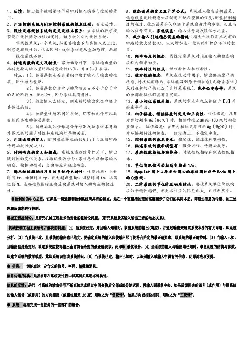
1、反馈:输出信号被测量环节引回到输入端参与控制的作用。
2、开环控制系统与闭环控制系统的根本区别:有无反馈。
3、线性及非线性系统的定义及根本区别:当系统的数学模型能用线性微分方程描述时,该系统的称为线性系统。
非线性系统:一个系统,如果其输出不与其输入成正比,则它是非线性的。
根本区别:线性系统遵从叠加原理,而非线性系统不然。
4、传递函数的定义及特点:零初始条件下,系统输出量的拉斯变换与输入量的拉斯变换的比值。
用G〔s〕表示。
特点:1〕、传递函数是否有量纲取决于输入与输出的性质,同性质无量纲。
2〕、传递函数分母中S的阶数必n不小于分子中的S的阶数m,既n=>m ,因为系统具有惯性。
3〕、假设输入已给定,则系统的输出完全取决于其传递函数。
4〕、物理量性质不同的系统,环节和元件可以具有相同类型的传递函数。
5〕、传递函数的分母与分子分别反映系统本身与外界无关的固有特性和系统同外界的关系。
5、开环函数的定义:前向通道传递函数G〔s〕与反馈回路传递函数H(s)之积。
6、时间响应的定义和组成:系统在激励信号作用下,输出随时间的变化关系。
按振动来源分为:零状态响应和零输入响应。
按振动性质:自由响应和强迫响应。
7、瞬态性能指标以及反映系统什么特性:性能指标:上升时间tr、峰值时间tp、最大超调量Mp、调整时间ts、振荡次数N。
这些性能指标主要反映系统对输入的响应的快速性。
8、稳态误差的定义及计算公式:系统进入稳态后的误差。
稳态误差反映稳态响应偏离系统希望值的程度。
衡量控制精度的程度。
稳态误差不仅取决于系统自身结构参数,而且与输入信号有关。
系统误差:输入信号与反馈信号之差。
9、减少输入引起稳态误差的措施:增大干扰作用点之前的回路的放大倍数K1,以及增加这一段回路中积分环节的数目。
10、频率响应的概念:线性定常系统对谐波输入的稳态响应称为频率响应。
11、频率特性的组成:幅频特性和相频特性。
12、稳定性的概念:系统在扰动作用下,输出偏离原平衡状态,待扰动消除后,系统能回到原平衡状态〔无静差系统〕或到达新的平衡状态〔有静差系统〕。
19春学期《自动控制原理Ⅰ》在线作业1最大超调量越大,说明系统过渡过程越不平稳。
A.是B.否正确答案:A调节时间的长短反映了系统动态响应过程的波动程度,它反映了系统的平稳性。
A.是B.否正确答案:BA.是B.否正确答案:A对于最小相位系统,相位裕度等于零的时候表示闭环系统处于临界稳定状态。
()A.是B.否正确答案:A开环对数频率特性的中频段反映了系统的稳定性和暂态性能。
()A.是B.否正确答案:A典型的非线性环节有继电器特性环节、饱和特性环节、不灵敏区特性环节等。
A.是B.否正确答案:A振荡次数越少,说明系统的平稳性越好。
A.是B.否正确答案:A系统结构图等效变换的原则是,换位前后的()保持不变。
A.输入信号B.输出信号C.反馈信号D.偏差信号正确答案:B上升时间指系统的输出量第一次达到输出稳态值所对应的时刻。
A.是B.否正确答案:A开环对数频率特性的低频段反映了系统的控制精度。
()A.是B.否正确答案:A在典型二阶系统中,当()时,系统是不稳定的。
A.AB.BC.CD.D正确答案:DA.是B.否正确答案:B典型二阶系统,()时为二阶工程最佳参数。
A.AB.BC.CD.D正确答案:B时滞环节在一定条件下可以近似为()A.比例环节B.积分环节C.微分环节D.惯性环节正确答案:D最大超调量反映了系统的平稳性。
A.是B.否正确答案:A自动控制系统按其主要元件的特性方程式的输入输出特性,可以分为线性系统和非线性系统。
A.是B.否正确答案:A频率特性可分解为相频特性和幅频特性。
()A.是B.否正确答案:A对于最小相位系统,相位裕度大于零的时候表示闭环系统是不稳定的。
()A.是B.否正确答案:B在典型二阶系统中,()时,系统是不稳定的。
A.过阻尼状态B.欠阻尼状态C.临界阻尼状态D.无阻尼状态正确答案:D最大超调量反映了系统的A.稳定性B.快速性C.平稳性D.准确性正确答案:C对于一般的控制系统,输出量的暂态过程中,下列哪种情况是稳定的A.持续振荡过程B.衰减振荡过程C.发散振荡过程D.等幅振荡过程正确答案:B振荡次数越多,说明系统的平稳性越好。
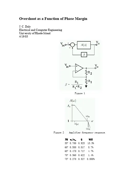
Overshoot as a Function of Phase MarginJ. C. DalyElectrical and Computer EngineeringUniversity of Rhode Island4/19/03Figure 1Figure 2 Amplifier frequency response.PM wt /weqQ%OS55o0.700 0.925 13.3% 60o0.580 0.817 8.7% 65o0.470 0.717 4.7% 70o0.360 0.622 1.4% 75o0.270 0.527 0.008%When an amplifier with a gain A(s) is put in afeedback loop as shown in Figure 1, the closed loop gain, V o /V in = A CL(1) The system is unstable when the loop gain, ß A(s), equals -1. That is, ß A(s) has a magnitude of one and a phase of -180degrees. An unstable system oscillates. A system close to being unstable has a large ringing overshoot in response to a step input.The phase margin is a measure of how close the phase of the loop gain is to -180 degrees, when the magnitude of the loop gain is one. The phase margin is the additional phase required to bring the phase of the loop gain to -180 degrees. Phase Margin = Phase of loop gain - (-180). The loop gain has a dominant pole at. Higher order poles can berepresented by an equivalent pole at . The amplifier is approximated by a function with two poles as shown in Equation 2.(2)Since for frequencies of interest where the loop gain magnitude is close to unity,(3)And,(4)(5)Defining ,Table IPM is the phase margin. w t is the unity gain frequency (rad/sec).w eq is the frequency of the equivalent higher order pole (rad/sec).Q is the system Quality factor.OS is the Over Shoot.(6)For frequencies of interest (frequencies close to the unity gain frequency), the amplifier gain can be written,(7)Plugging Equation 7 into Equation 1 results in the following expression for the closed loop gain.(8)Equation 8 is the transfer function for a second order system. The general form for the response of a second order system, where system properties are described by its Q and resonant frequence w o , is shown in Equation 10.(9)By comparing Equation 8 to Equation 9 we can get an expression for the resonant frequency and Q of the amplifier closed loop gain. (Equate coefficients of like powers of s in the dominators.)(10)(11)The loop gain is the feedback factor ß multiplied by the amplifier gain A(s).(12)The phase margin is a function of the phase of the loop gain at the frequency where the magnitude of the loop gain is unity.(13)where is the loop gain unity gain frequency. It follows from Equations 12 and 13 that,(14)Also, solving for w ta and dividing by w eq ,(15)It follows from Equations 11 and 15 that,(16)The phase of the loop gain (Equation 13) is.Phase of loop gain(17)The phase margin is the additional phase required to bring the phase of the loop gain to -180 degrees.Phase Margin = Phase of loop gain - (-180).Phase Margin(18)A well known property of second order systems is that the percent overshoot is a function of the Q and is given by,(19)Both phase margin (Equation 18) and Q (Equation 16) are a function of wt/weq . This allows us to use Equation 19 to create tables and plots of percent overshoot as a function of phase margin. As shown in Figures 3 and 4, and in Table I.Figure 3 Overshoot as a functionof phase margin. Plot generatedusingMATLAB code.Figure 4 Q as a function of phase margin. Plot generated using MATLAB code.。

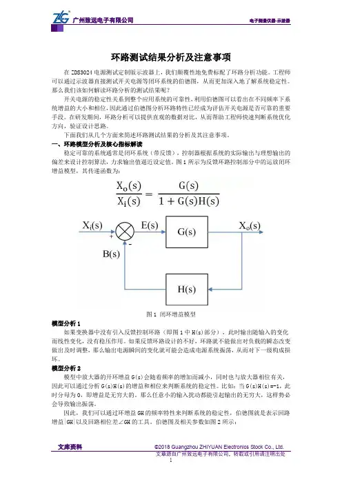
环路测试结果分析及注意事项在ZDS3024电源测试定制版示波器上,我们颠覆性地免费标配了环路分析功能。
工程师可以通过示波器直接测试开关电源等闭环系统的伯德图,从而更加深入地了解系统稳定性。
那么我们该如何解读环路分析的测试结果呢?开关电源的稳定性关系到整个应用系统的可靠性,利用伯德图可以看出在不同频率下系统增益的大小和相位,因此通过伯德图分析环路特性已经成为评估开关电源是否可靠的重要手段。
在研发期间,环路分析可以提供直观的数据对比,从而帮助工程师快速判断系统优化方向,验证设计思路。
下面我们从几个方面来简述环路测试结果的分析及其注意事项。
一、环路模型分析及核心指标解读稳定可靠的系统通常是闭环系统(带反馈),控制器根据系统的实际输出与理想输出的偏差来设计控制算法,力求输出值逼近设定值。
图1所示为反馈环路控制部分中的运放闭环增益模型,其传递函数为:图1 闭环增益模型模型分析1如果变换器中没有引入反馈控制环路(即图1中H(s)部分),此时输出随输入的变化而线性变化,没有稳压作用。
如果反馈环路设计的不好,环路就不能做出对负载的瞬态改变做出及时调整,那么输出电源瞬间的变化就可能会造成电源系统振荡,从而对下一级构成损坏。
模型分析2模型中放大器的开环增益G(s)会随着频率的增加而减小,同时也与放大器相位有关,因此可以通过分析G(s)H(s)的增益和相位来判断系统的稳定性。
比如:当G(s)H(s)=-1,此时分母为0,即增益是无穷大的。
那么任意小的输入扰动都能引起输出的无穷大,这样势必会导致输出振荡。
因此,我们可以通过环增益GH的频率特性来判断系统的稳定性,伯德图就是表示回路增益|GH|以及回路相位差∠GH的工具。
伯德图及相关参数如图2所示:图2 伯德图及相关参数伯德图有以下3个核心指标:●穿越频点:增益为0dB时对应的频率;●相位裕度:增益为0dB时对应的相位差;●增益裕度:相位为0°时对应的增益差。
由此可见,闭环系统的稳定性可以通过伯德图中的相位裕度,增益裕度,穿越频点来衡量。
江南大学现代远程教育第三阶段测试卷考试科目:《机械工程控制基础》(第五章、第六章)(总分100分)时间:90分钟学习中心(教学点)批次:层次:专业:学号:身份证号:姓名:得分:一、单项选择题(本题共15小题,每小题2分,共30分。
)1、已知系统特征方程为 3s4+10s3+5s2+s+2=0,则该系统包含正实部特征根的个数为()。
A、0B、1C、2D、32、劳斯判据用()来判定系统的稳定性。
A、系统特征方程B、开环传递函数C、系统频率特性的Nyquist图D、系统开环频率特性的Nyquist图3、已知系统特征方程为 s4+s3+4s2+6s+9=0,则该系统()。
A、稳定B、不稳定C、临界稳定D、无法判断4、延时环节串联在闭环系统的前向通道时,系统稳定性()。
A、变好B、变坏C、不会改变D、时好时坏5、开环传递函数 G K(s)、闭环传递函数 G B(s)和辅助函数 F(s)=1+G K(s)三者之间的关系为()。
A、G K(s)绕(-1,j0)点的圈数就是G K(s)绕原点的圈数B、G K(s)绕原点的圈数就是G B(s)绕(-1,j0)点的圈数C、G K(s)绕(-1,j0)点的圈数就是F(s)=1+G K(s)绕原点的圈数D、G K(s)绕原点的圈数就是F(s)=1+G K(s)绕(-1,j0)点的圈数6、已知开环稳定的系统,其开环频率特性的Nyquist图如图所示,则该闭环系统()。
A、稳定B、不稳定C、临界稳定D、与系统初始状态有关7、设单位反馈系统的开环传递函数为 G K(s)= K/[s(s+1)(s+3)],则此系统稳定的K值范围为()。
A、K<0B、K>0C、2>K>0D、12>K>08、对于一阶系统,时间常数越大,则系统()。
A、系统瞬态过程越长B、系统瞬态过程越短C、稳态误差越小D、稳态误差越大9、系统稳定的充要条件()。
A、幅值裕度大于0分贝B、相位裕度大于0C、幅值裕度大于0分贝,且相位裕度大于0D、幅值裕度大于0分贝,或相位裕度大于010、以下方法可增加系统相对稳定性的是()。
第一套一、单项选择填空(每小题4分,共20分) 1. 系统不稳定时,其稳定误差为( )1)+∞ 2)-∞ 3)0 4)以上都不对 2. 2-1-2型渐近对数幅频特性描述的闭环系统一定( )1)稳定 2)不稳定 3)条件稳定 4)说不清 3. 由纯积分环节经单位反馈而形成的闭环系统超调量为( ) 1)0 2)16.3% 3)无超量 4)以上都对 4. 描述函数描述了( )系统的性能。
1)非线性系统 2)本质非线性系统 3)线性、非线性系统 4)以上都错 5. 采样周期为( )的系统是连续系统。
1)0 2)∞ 3)需经严格证明 4)以上都错 二、简化结构图求传递函数C(s)/R(s) (每小题8分,共16分)1.2.三、单位负反馈系统的零初始条件下的单位阶跃响应为 (每小题5分,共20分)1. 析开环、闭环稳定性;2. 超调量;3. 求Δ=±0.02L(∞)时,调节时间;4. 求阶跃响应时的稳态误差。
四、单位负反馈系统的开环传递函数为 (每小题8分,共16分)1. 绘制闭环根轨迹图;2. 决定闭环稳定的k 1的范围。
五、单位负反馈系统开环传递函数为 (每小题8分,共16分)1. 绘制开环伯德图;2. 分析闭环稳定性。
0≥ +-=--t tg t e t C t )220sin(1)(15)1)(3()(1++=s s s k s G )1()(21++=s s s k s G第四套一、对自动控制系统基本的性能要求是什么?其中最基本的要求是什么?(5分)二、已知系统结构图如图1所示。
(20分) 1)求传递函数E(s)/R(s) 和 E(s)/N(s)。
2)若要消除干扰对误差的影响(即E(s)/N(s)=0),问G 0(s)=?图1三、已知系统结构图如图2所示,要求系统阻尼比0.6ζ=。
(20分) 1)确定K f 值并计算动态性能指标t p ,σ%,t s ; (提示:p dt πω=,%p e σ=4s nt ζω=)2)求在r (t )=t ,作用下系统的稳态误差。
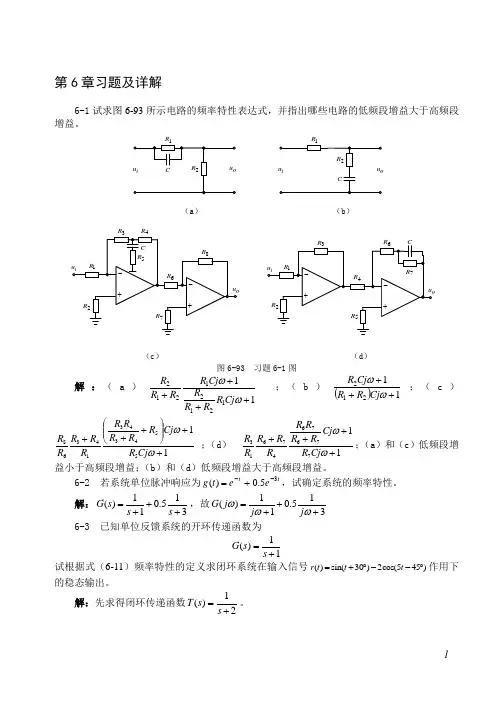
第6章习题及详解6-1 试求图6-93所示电路的频率特性表达式,并指出哪些电路的低频段增益大于高频段增益。
(a ) (b )R R(c ) (d )图6-93 习题6-1图解:(a )1112121212++++ωωCj R R R R Cj R R R R ;(b )()11212+++ωωCj R R Cj R ;(c )1155434314368++⎪⎪⎭⎫ ⎝⎛+++ωωCj R Cj R R R R R R R R R R ;(d ) 117767647613++++ωωCj R Cj R R R R R R R R R ;(a )和(c )低频段增益小于高频段增益;(b )和(d )低频段增益大于高频段增益。
6-2 若系统单位脉冲响应为t t e e t g 35.0)(--+=,试确定系统的频率特性。
解:315.011)(+++=s s s G ,故315.011)(+++=ωωωj j j G 6-3 已知单位反馈系统的开环传递函数为11)(+=s s G 试根据式(6-11)频率特性的定义求闭环系统在输入信号()sin(30)2cos(545)r t t t =+︒--︒作用下的稳态输出。
解:先求得闭环传递函数21)(+=s s T 。
(1)1=ω,447.055211)1(==+=j j T ,︒-=-=∠56.2621arctan )1(j T 。
(2)5=ω,186.02929251)5(==+=j j T ,︒-=-=∠20.6825arctan )5(j T 。
故)2.1135cos(372.0)44.3sin(447.0)(︒--︒+=∞→t t t y t 。
6-4 某对象传递函数为s e Ts s G τ-+=11)( 试求:(1) 该对象在输入()sin()u t t ω=作用下输出的表达式,并指出哪部分是瞬态分量; (2) 分析T 和τ增大对瞬态分量和稳态分量的影响;(3) 很多化工过程对象的T 和τ都很大,通过实验方法测定对象的频率特性需要很长时间,试解释其原因。
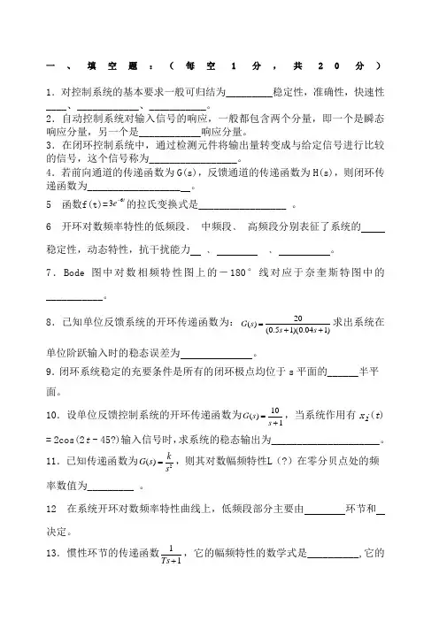
一、填空题:(每空1分,共20分)1.对控制系统的基本要求一般可归结为_________稳定性,准确性,快速性____、____________、___________。
2.自动控制系统对输入信号的响应,一般都包含两个分量,即一个是瞬态响应分量,另一个是____________响应分量。
3.在闭环控制系统中,通过检测元件将输出量转变成与给定信号进行比较的信号,这个信号称为_________________。
4.若前向通道的传递函数为G(s),反馈通道的传递函数为H(s),则闭环传递函数为__________________ 。
5 函数f(t)=te 63-的拉氏变换式是_________________ 。
6 开环对数频率特性的低频段﹑ 中频段﹑ 高频段分别表征了系统的稳定性,动态特性,抗干扰能力 ﹑ ﹑ 。
7.Bode 图中对数相频特性图上的-180°线对应于奈奎斯特图中的___________。
8.已知单位反馈系统的开环传递函数为:20()(0.51)(0.041)G s s s =++求出系统在单位阶跃输入时的稳态误差为 。
9.闭环系统稳定的充要条件是所有的闭环极点均位于s 平面的______半平面。
10.设单位反馈控制系统的开环传递函数为10()1G s s =+,当系统作用有x i (t ) = 2cos(2t - 45?)输入信号时,求系统的稳态输出为_____________________。
11.已知传递函数为2()k G s s=,则其对数幅频特性L (?)在零分贝点处的频率数值为_________ 。
12 在系统开环对数频率特性曲线上,低频段部分主要由 环节和 决定。
13.惯性环节的传递函数11+Ts ,它的幅频特性的数学式是__________,它的相频特性的数学式是____________________。
14.已知系统的单位阶跃响应为()1t t o x t te e --=+-,则系统的脉冲脉冲响应为__________。
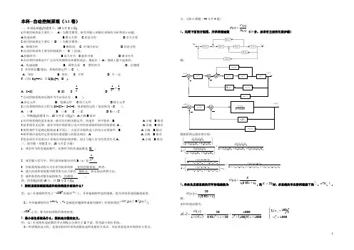
本科--自动控制原理(A1卷)一、单项选择题(每题2分,16分共8小题)1.经典控制理论主要以( A )为数学模型,研究单输入单输出系统的分析和设计问题。
A.传递函数 B.微分方程 C.状态方程 D.差分方程2.现代控制理论主要以( D )为数学模型。
A .频域分析 B.根轨迹 C. 时域分析法 D.状态方程 3.自动控制系统主要有控制器和( C )组成。
A.检测环节B.放大环节C.被控对象D.调节环节 4.在经典控制理论中广泛应用的频率法和根轨迹法,都是在( A )基础上建立起来的。
A .传递函数 B .频率分析 C .惯性环节 D .伯德图 5. 开环增益K 增加,系统的稳定性( C )。
A .变好 B. 变坏 C. 不变 D. 不一定 6. 已知 f(t)=t+1,其L[f(t)]=( D )。
A .S+S2 B. S2 C. 1S D. 211SS + 7.自动控制系统的反馈环节中必须具有( B )。
A.给定元件 B .检测元件 C.放大元件 D.执行元件 8.已知系统的特征方程为S3+S2+τS+5=0,则系统稳定的τ值范围为(C )。
A .τ>0B. τ<0C. τ>5D. 0<τ<5 二、判断题(每题2分,10分共5小题)注:A.正确B.错误1.对控制系统的基本要求一般可以归纳为稳定性、快速性 和平稳性。
B A.正确 B.错误2.按系统有无反馈,通常可将控制系统分为开环控制系统和闭环控制系统 A 。
A.正确 B.错误3.相角条件不是确定根轨迹S 平面上一点是否在根轨迹上的充分必要条件。
B A.正确 B.错误4.频率响应是线性定常系统对谐波输入的稳态响应。
A A.正确 B.错误5.稳态误差不仅取决于系统自身的结构参数,而且与输入信号的类型有关A 。
A.正确 B.错误 三、填空题(每题2分,10分共5小题)1.典型环节的传递函数中,比例环节的传递函数是 K 。
1. 闭环控制系统又称为反馈控制系统。
2.对控制系统的首要要求是系统具有稳定性。
3. 若要全面地评价系统的相对稳定性,需要同时根据相位裕量和幅值裕量来做出判断。
4. 系统主反馈回路中最常见的校正形式是串联校正和反馈校正。
5. 某典型环节的传递函数是G(s)=1/(s+2),则系统的时间常数是 0.5。
6. 若要求系统的快速性好,则闭环极点应距虚轴越远越好。
7. 在扰动作用点与偏差信号之间加上积分环节能使静态误差降为0。
8.二阶系统的传递函数G(s)=4/(s 2+2s+4),其固有频率ωn =2。
9. 远离虚轴的闭环极点对瞬态响应的影响很小。
10.为满足机电系统的高动态特性,机械传动的各个分系统的谐振频率应远高于机电系统的设计截止频率。
11.当奈奎斯特图逆时针从第二象限越过负实轴到第三象限去时称为正穿越。
12.对于最小相位系统一般只要知道系统的 开环幅频特性就可以判断其稳定性。
13.判断一个闭环线性控制系统是否稳定,在时域分析中采用劳斯判据;在频域分析中采用奈奎斯特判据。
14.若某系统的单位脉冲响应为0.20.5()105t t g t e e --=+,则该系统的传递函数G(s)为10/(s+0.2)+5/(s+0.5)。
1. 根据采用的信号处理技术的不同,控制系统分为模拟控制系统和数字控制系统。
2. 若系统的传递函数在右半S 平面上没有零点和极点,则该系统称作最小相位系统。
3. 输入相同时,系统型次越高,稳态误差越小。
4. 延迟环节不改变系统的幅频特性,仅使相频特性发生变化。
5. PID 调节中的“P”指的是比例控制器。
6. 用频率法研究控制系统时,采用的图示法分为极坐标图示法和对数坐标图示法。
7. 一般开环频率特性的低频段表征了闭环系统的稳态性能。
8. 复合控制有两种基本形式:即按输入的前馈复合控制和按扰动的前馈复合控制。
9. 奈奎斯特图中当ω等于截止频率时,相频特性距-π线的相位差叫相位裕量。
一、填空题(每空 1 分,共15分)1、反馈控制又称偏差控制,其控制作用是通过给定值与反馈量的差值进行的。
2、复合控制有两种基本形式:即按输入的前馈复合控制和按扰动的前馈复合控制。
3、两个传递函数分别为G 1(s)与G 2(s)的环节,以并联方式连接,其等效传递函数为()G s ,则G(s)为G1(s)+G2(s)(用G 1(s)与G 2(s) 表示)。
4、典型二阶系统极点分布如图1所示,则无阻尼自然频率=nω,阻尼比=ξ,0.7072= 该系统的特征方程为2220s s ++= ,该系统的单位阶跃响应曲线为衰减振荡。
5、若某系统的单位脉冲响应为0.20.5()105t t g t e e --=+,则该系统的传递函数G(s)为1050.20.5s s s s+++。
6、根轨迹起始于开环极点,终止于开环零点。
7、设某最小相位系统的相频特性为101()()90()tg tg T ϕωτωω--=--,则该系统的开环传递函数为(1)(1)K s s Ts τ++。
8、PI 控制器的输入-输出关系的时域表达式是1()[()()]p u t K e t e t dt T =+⎰, 其相应的传递函数为1[1]p K Ts +,由于积分环节的引入,可以改善系统的稳态性能。
1、在水箱水温控制系统中,受控对象为水箱,被控量为水温。
2、自动控制系统有两种基本控制方式,当控制装置与受控对象之间只有顺向作用而无反向联系时,称为开环控制系统;当控制装置与受控对象之间不但有顺向作用而且还有反向联系时,称为闭环控制系统;含有测速发电机的电动机速度控制系统,属于闭环控制系统。
3、稳定是对控制系统最基本的要求,若一个控制系统的响应曲线为衰减振荡,则该系统稳定。
判断一个闭环线性控制系统是否稳定,在时域分析中采用劳斯判据;在频域分析中采用奈奎斯特判据。
4、传递函数是指在零初始条件下、线性定常控制系统的输出拉氏变换与输入拉氏变换之比。
自动控制原理复习题(二)一、选择题1、下列串联校正装置的传递函数中,能在1c ω=处提供最大相位超前角的是:A. 1011s s ++C. 210.51s s ++B. 1010.11s s ++ D. 0.11101s s ++2、一阶系统的闭环极点越靠近S 平面原点:A. 准确度越高 C. 响应速度越快B. 准确度越低 D. 响应速度越慢3、已知系统的传递函数为1s Ke TS τ-+,其幅频特性()G j ω应为: A. 1Ke T τω-+τω-B. 1Ke T τωω-+4、梅逊公式主要用来( )A. 判断稳定性 C. 求系统的传递函数B. 计算输入误差 D. 求系统的根轨迹5、 适合应用传递函数描述的系统是: A. 单输入,单输出的线性定常系统;B. 单输入,单输出的线性时变系统;C. 单输入,单输出的定常系统;D. 非线性系统。
6、对于代表两个或两个以上输入信号进行( )的元件又称比较器。
A. 微分 C. 加减B. 相乘 D. 相除 7、直接对控制对象进行操作的元件称为( )A. 比较元件C. 执行元件B.给定元件D. 放大元件8、二阶欠阻尼系统的性能指标中只与阻尼比有关的是()A. 上升时间C. 调整时间B.峰值时间D. 最大超调量9、在用实验法求取系统的幅频特性时,一般是通过改变输入信号的()来求得输出信号的幅值。
A. 相位C. 稳定裕量B.频率D. 时间常数10、已知二阶系统单位阶跃响应曲线呈现出等幅振荡,则其阻尼比可能为()A. 0.707 C. 1B.0.6 D. 011、非单位反馈系统,其前向通道传递函数为G(S),反馈通道传递函数为H(S),则输入端定义的误差E(S)与输出端定义的误差*()E S之间有如下关系:A.* ()()() E S H S E S=⋅C.*()()()()E S G S H S E S=⋅⋅B.*()()()E S H S E S=⋅D.*()()()()E S G S H S E S=⋅⋅12、若两个系统的根轨迹相同,则有相同的:A. 闭环零点和极点C. 闭环极点B.开环零点D. 阶跃响应13、已知下列负反馈系统的开环传递函数,应画零度根轨迹的是:A.*(2) (1) K s s s-+C.*2(31)Ks s s+-B.*(1)(5Ks s s-+)D.*(1)(2)K ss s--14、闭环系统的动态性能主要取决于开环对数幅频特性的:A. 低频段C. 高频段B.开环增益D. 中频段15、系统特征方程式的所有根均在根平面的左半部分是系统稳定的()A. 充分条件C. 充分必要条件B.必要条件D. 以上都不是16、以下关于系统稳态误差的概念正确的是( C )A. 它只决定于系统的结构和参数B.它只决定于系统的输入和干扰C. 与系统的结构和参数、输入和干扰有关D. 它始终为0非线性系统17、当输入为单位加速度且系统为单位反馈时,对于I型系统其稳态误差为()A. 0 C. 1/kB.0.1/k D.18、开环控制的特征是()A. 系统无执行环节C. 系统无反馈环节B.系统无给定环节D. 系统无放大环节19、若已知某串联校正装置的传递函数为,则它是一种()A. 相位滞后校正C. 微分调节器B.相位超前校正D. 积分调节器20、在信号流图中,只有()不用节点表示。
自动控制原理简答题自动控制原理简答题 47、传递函数:传递函数是指在零初始条件下,系统输出量的拉式变换与系统输入量的拉式变换之比。
48、系统校正:为了使系统到达我们的要求,给系统参加特定的环节,使系统到达我们的要求,这个过程叫系统校正。
49、主导极点:假如系统闭环极点中有一个极点或一对复数极点据虚轴最近且附近没有其他闭环零点,那么它在响应中起主导作用称为主导极点。
51、状态转移矩阵:,描绘系统从某一初始时刻向任一时刻的转移。
52、峰值时间:系统输出超过稳态值到达第一个峰值所需的时间为峰值时间。
53、动态构造图:把系统中所有环节或元件的传递函数填在系统原理方块图的方块中,并把相应的输入输出信号分别以拉氏变换来表示从而得到的传递函数方块图就称为动态构造图。
54、根轨迹的渐近线:当开环极点数 n 大于开环零点数m 时,系统有n-m 条根轨迹终止于 S 平面的无穷远处,且它们交于实轴上的一点,这 n-m 条根轨迹变化趋向的直线叫做根轨迹的渐近线。
55、脉冲传递函数:零初始条件下,输出离散时间信号的z变换与输入离散信号的变换之比,即。
56、Nyquist判据〔或奈氏判据〕:当ω由-∞变化到+∞时, Nyquist曲线〔极坐标图〕逆时针包围〔-1,j0〕点的圈数N,等于系统G(s)H(s)位于s右半平面的极点数P ,即N=P,那么闭环系统稳定;否那么〔N≠P〕闭环系统不稳定,且闭环系统位于s右半平面的极点数Z为:Z=∣P-N∣ 57、程序控制系统: 输入信号是一个的函数,系统的控制过程按预定的程序进展,要求被控量能迅速准确地复现输入,这样的自动控制系统称为程序控制系统。
58、稳态误差:对单位负反应系统,当时间t趋于无穷大时,系统对输入信号响应的实际值与期望值〔即输入量〕之差的极限值,称为稳态误差,它反映系统复现输入信号的〔稳态〕精度。
59、尼柯尔斯图〔Nichocls图〕:将对数幅频特性和对数相频特性画在一个图上,即以〔度〕为线性分度的横轴,以l(ω)=20lgA(ω)〔db〕为线性分度的纵轴,以ω为参变量绘制的φ(ω) 曲线,称为对数幅相频率特性,或称作尼柯尔斯图〔Nichols图〕60、零阶保持器:零阶保持器是将离散信号恢复到相应的连续信号的环节,它把采样时刻的采样值恒定不变地保持〔或外推〕到下一采样时刻。
相位裕量过冲过阻欠阻
相位裕量、过冲、过阻和欠阻都是控制系统工程中常见的概念,它们在系统分析和设计中起着重要的作用。
让我逐个解释:
相位裕量是指系统在闭环控制下,对于相位变化的容忍程度。
它反映了系统的稳定性能,通常用来评估系统的相位裕度,即系统
在闭环控制下能够容忍多大程度的相位变化而不失稳定性。
相位裕
量越大,系统对相位变化的容忍能力越强,稳定性越好。
过冲是指系统在响应过程中超出稳态值的最大偏差。
在控制系
统中,过冲通常是由于系统具有较高的控制增益或者较快的响应速
度而导致的,过大的过冲会影响系统的稳定性和精度,因此需要在
系统设计中进行合理的抑制。
过阻是指系统在响应过程中,由于阻尼过大而导致的响应速度
过慢,使得系统的超调量变小,但响应时间变长,甚至导致不稳定。
过阻会影响系统的动态性能和稳定性,因此需要在系统设计中进行
合理的调节。
欠阻是指系统在响应过程中,由于阻尼不足而导致的振荡或者
过冲现象。
欠阻会使系统的响应过程出现振荡甚至不稳定,因此也需要在系统设计中进行合理的调节。
综上所述,相位裕量、过冲、过阻和欠阻都是控制系统设计和分析中需要考虑的重要因素,合理的设计和调节可以保证系统具有良好的稳定性和动态性能。
在实际工程中,工程师需要综合考虑这些因素,以达到系统设计的要求。
自动控制原理相位裕量-回复自动控制原理相位裕量是控制理论中的一个重要概念,用于评估系统的稳定性和鲁棒性。
相位裕量指的是系统的相位特性与临界稳定边界之间的差距。
在控制系统设计中,相位裕量是一个关键参数,其值应该足够大,以确保系统的稳定性和性能。
要了解相位裕量,首先需要了解系统的频率响应特性。
在控制系统中,频率响应描述了系统对不同频率输入信号的响应。
频率响应通常通过幅频特性和相频特性来表示。
其中,幅频特性描述了系统对输入信号的幅度放大或衰减情况,而相频特性描述了系统对输入信号的相位延迟或提前情况。
在频域中,相位裕量指的是系统的相位特性与临界稳定边界之间的相位差。
临界稳定边界是指系统刚好处于稳定与不稳定之间的边界,在该边界上系统的增益较低,相位较大。
相位裕量的值越大,表示系统在临界稳定边界处的相位差越大,系统的稳定性和鲁棒性也越好。
那么如何计算相位裕量呢?常见的计算方法有两种:增益裕量法和封闭环极点分布法。
增益裕量法是通过测量系统的幅频特性曲线和相频特性曲线,来计算相位裕量的值。
这种方法需要使用频率响应测量仪器或者模拟计算的方法,对系统进行测试。
通过测量系统在临界稳定边界处的相位差,可以得到相位裕量的值。
封闭环极点分布法是一种基于极点分布的方法,通过对系统的开环传递函数进行极点分析,来评估系统的相位裕量。
该方法可以通过计算系统的相位裕量角度来确定相位裕量的值。
通常,相位裕量的值应该大于45度,才能确保系统的稳定性和性能。
相位裕量在控制系统设计中扮演着至关重要的角色。
一个合理的相位裕量值可以提高系统的稳定性,并保证系统在干扰和不确定性的情况下具有较好的鲁棒性。
相位裕量的大小与系统的增益裕量和带宽有关。
在实际应用中,设计师通常会根据系统的需求和性能要求来确定适当的相位裕量值。
总之,相位裕量是控制系统设计过程中一个重要的概念,用于评估系统的稳定性和鲁棒性。
合理的相位裕量值可以保证系统具有良好的性能,并在干扰和不确定性的情况下保持稳定。
Overshoot as a Function of Phase Margin
J. C. Daly
Electrical and Computer Engineering
University of Rhode Island
4/19/03
Figure 1
Figure 2 Amplifier frequency response.
PM w
t /w
eq
Q%OS
55o0.700 0.925 13.3% 60o0.580 0.817 8.7% 65o0.470 0.717 4.7% 70o0.360 0.622 1.4% 75o0.270 0.527 0.008%
When an amplifier with a gain A(s) is put in a
feedback loop as shown in Figure 1, the closed loop gain, V o /V in = A CL
(1)
The system is unstable when the loop gain, ß A(s), equals -1. That is, ß A(s) has a magnitude of one and a phase of -180
degrees. An unstable system oscillates. A system close to being unstable has a large ringing overshoot in response to a step input.
The phase margin is a measure of how close the phase of the loop gain is to -180 degrees, when the magnitude of the loop gain is one. The phase margin is the additional phase required to bring the phase of the loop gain to -180 degrees. Phase Margin = Phase of loop gain - (-180). The loop gain has a dominant pole at
. Higher order poles can be
represented by an equivalent pole at . The amplifier is approximated by a function with two poles as shown in Equation 2.
(2)
Since for frequencies of interest where the loop gain magnitude is close to unity,
(3)
And,
(4)
(5)
Defining ,
Table I
• PM is the phase margin. • w t is the unity gain frequency (rad/sec).
• w eq is the frequency of the equivalent higher order pole (rad/sec).
• Q is the system Quality factor.
• OS is the Over Shoot.
(6)
For frequencies of interest (frequencies close to the unity gain frequency), the amplifier gain can be written,
(7)
Plugging Equation 7 into Equation 1 results in the following expression for the closed loop gain.
(8)
Equation 8 is the transfer function for a second order system. The general form for the response of a second order system, where system properties are described by its Q and resonant frequence w o, is shown in Equation 10.
(9)
By comparing Equation 8 to Equation 9 we can get an expression for the resonant frequency and Q of the amplifier closed loop gain. (Equate coefficients of like powers of s in the dominators.)
(10)
(11)
The loop gain is the feedback factor ß multiplied by the amplifier gain A(s).
(12)
The phase margin is a function of the phase of the loop gain at the frequency where the magnitude of the loop gain is unity.
(13)
where is the loop gain unity gain frequency. It follows from Equations 12 and 13 that,
(14)
Also, solving for w ta and dividing by w eq,
(15)
It follows from Equations 11 and 15 that,
(16)
The phase of the loop gain (Equation 13) is.
Phase of loop gain(17)
The phase margin is the additional phase required to bring the phase of the loop gain to -180 degrees.
Phase Margin = Phase of loop gain - (-180).
Phase Margin(18)
A well known property of second order systems is that the percent overshoot is a function of the Q and is given by,
(19)
Both phase margin (Equation 18) and Q (Equation 16) are a function of w t / w eq. This allows us to use Equation 19 to create tables and plots of percent overshoot as a function of phase margin. As shown in Figures 3 and 4, and in Table I.
Figure 3 Overshoot as a function
of phase margin.
Plot generated using MATLAB code.Figure 4 Q as a function of phase margin.
Plot generated using MATLAB code.。