基于BELLHOP的水声信道时变模型

基于射线模型的典型海底地形下的声传播海洋中检测、通信、定位和导航主要利用声波。

声波是目前水下信息传输的主要载体。

文章基于射线模型对深海环境下四种典型海底地形声传播展开研究。

仿真结果表明，可利用海底地形对声波的反射和折射效应，获得声源达到空间任意位置的声线传播轨迹和传播损失，基于射线模型的声传播研究可为实际海洋环境下的水下信息传输以及探测提供技术支持。

标签：典型海底地形；射线模型；声线传播1 概述在海洋环境中，海底地形是水声传播的下边界，不同的海底地形对水下声传播有着重要的影响。

研究海底地形与声传播的关系对水下探测、定位和信息传输等有着极其重要的作用。

射线模型在声传播的研究中使用比较广泛，该模型应用简单直观、计算速度快。

射线模型计算出声场的传播损失以及声线的传播路径等多种数据，是声场研究的一种有效方法。

射线模型在处理声线的会聚区与影区、声线的传播路径等方面要优于简正波模型。

在射线模型中，Bellhop模型引入高斯波束跟踪法，在处理声线完全影区和能量焦散等问题方面与传统模型相比有非常明显地改进。

需要说明的是，Bellhop模型在计算高频率的声传播时，结果与实际比较接近，效果比较好，并且随着研究的不断深入，通过对Bellhop模型的处理和改进，在低频率的声传播研究中，也能够得到较好的结果[1]。

本文针对典型声速剖面下，利用Bellhop模型实现了深海环境中，四种典型海底地形的水下声学仿真实验，可为水下信息传输和探测提供理论的研究依据。

2 射线理论模型在射线模型中，声场中的能量是靠声线来传播的，声源发出的声线在信道中按照一定的路径传播后到达接收点，接收点所接收到的声能是所有到达该点的声线能量之和。

因为不同的声线有不同的传播路径，因此到达接收点的相位和时间也有所不同。

所有声线携带的能量是守恒的，经过传播过程中的扩展损失和吸收损失后，到达接收点的能量会有衰减，但是通过对传播损失的规律的研究，可以确定到达接收点的声线强度。

水声通信中信道建模方法研究随着科技的不断发展，水声通信作为一种非常重要的通信方式，正在越来越广泛地应用于军事、海底能源开发、海底地质勘探和海洋生态环境监测等领域。

但是，由于水声信道具有高时变性、多径效应、多变的海况环境等特点，使得水声通信信号传输的可靠性和质量受到了很大的制约，因此需要对水声信道进行建模和研究，以便更好地使用该通信方式。

1. 水声信道特点水声信道具有很高的时变性和多径效应。

这是因为水声信号在水中传输会被海水中的声音速度、密度和压力等参数影响，这些参数又与海洋动态环境密切相关，而海洋动态环境又缺乏规律性。

因此，水声信道中的信号会发生衰减、时延扩散、相位扭曲等现象。

另外，由于水声信号需要穿越水面和海底两个不同介质，因此还会发生反射、折射等多径效应。

2. 水声信道建模方法2.1 统计建模方法统计建模方法是利用概率和统计学方法来描述水声信道的特性，主要包括分布模型、随机过程模型、卡尔曼滤波模型等。

其中，分布模型利用概率密度函数来描述水声信号的时变性和多径效应，通常使用的分布模型有高斯分布模型、瑞利分布模型、约翰尼斯分布模型等。

随机过程模型则是利用随机过程来描述信号的统计特性，通常使用的随机过程模型包括高斯白噪声模型、马尔可夫模型、欧拉马尔柯夫模型等。

卡尔曼滤波模型则是利用卡尔曼滤波算法来对信道进行建模，可以有效地预测信号的时变性和多径效应。

2.2 物理建模方法物理建模方法是利用物理原理和实验数据来描述水声信道的特性，通常包括时频域建模方法、波浪算法建模方法等。

时频域建模方法利用时频分析技术对信道进行建模，通常使用的方法有傅里叶分析法、小波分析法、能量子空间法等。

波浪算法建模方法则是利用海洋波浪运动模拟水声信道的变化，通常使用的方法有海洋波浪模型、海洋动态模型等。

3. 信道建模方法的比较和选择在实际应用中，选择适合的信道建模方法对于提高水声通信系统的性能和可靠性至关重要。

一般来讲，物理建模方法更加贴近实际应用环境，具有更好的准确性和可预测性。

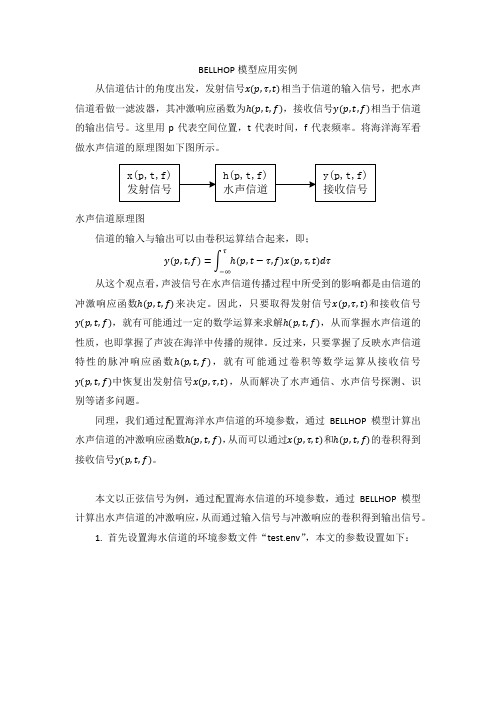
BELLHOP模型应用实例从信道估计的角度出发，发射信号x(p,τ,t)相当于信道的输入信号，把水声信道看做一滤波器，其冲激响应函数为ℎ(p,t,f)，接收信号y(p,t,f)相当于信道的输出信号。

这里用p代表空间位置，t代表时间，f代表频率。

将海洋海军看做水声信道的原理图如下图所示。

水声信道原理图信道的输入与输出可以由卷积运算结合起来，即；τy(p,t,f)=∫ℎ(p,t−τ,f)x(p,τ,t)dτ−∞从这个观点看，声波信号在水声信道传播过程中所受到的影响都是由信道的冲激响应函数ℎ(p,t,f)来决定。

因此，只要取得发射信号x(p,τ,t)和接收信号y(p,t,f)，就有可能通过一定的数学运算来求解ℎ(p,t,f)，从而掌握水声信道的性质，也即掌握了声波在海洋中传播的规律。

反过来，只要掌握了反映水声信道特性的脉冲响应函数ℎ(p,t,f)，就有可能通过卷积等数学运算从接收信号y(p,t,f)中恢复出发射信号x(p,τ,t)，从而解决了水声通信、水声信号探测、识别等诸多问题。

同理，我们通过配置海洋水声信道的环境参数，通过BELLHOP模型计算出水声信道的冲激响应函数ℎ(p,t,f)，从而可以通过x(p,τ,t)和ℎ(p,t,f)的卷积得到接收信号y(p,t,f)。

本文以正弦信号为例，通过配置海水信道的环境参数，通过BELLHOP模型计算出水声信道的冲激响应，从而通过输入信号与冲激响应的卷积得到输出信号。

1. 首先设置海水信道的环境参数文件“test.env”，本文的参数设置如下：在matlab 的命令行操作如下： >>bellhop 'test'<ENTER>生成“test.arr ”文件，读取“test.arr ”文件，绘制冲激响应如下图所示：2. 编写matlab 程序，计算输出信号。

1）参数设置：相对时延/s归一化幅度归一化冲激响应2）创建输入信号：3）读取“test.arr”文件，获取所需的幅度和时延：4）对单位冲激响应进行采样，并与输入信号做卷积，得到输出信号：5）绘制发送与接收信号波形：发送与接收信号波形如下图所示：对单位冲激响应采样的函数：00.050.10.150.2发送信号时间/s 幅值(V )5.255.35.355.4 5.45 5.54接收到的信号时间/s幅值(V )。

第1"卷第1期2019年2月指挥信息系统与技术Command Information System and TechnologyVol. 10 No.1Feb.2019•实践与应用•do# 10. 15908". cnki.cist.2019. 01. 015基于B E L L H O P模型的水中目标回波亮点特征建模与分析"崔化超晏谢飞(中国电子科技集团公司第二十八研究所南京210007)摘要：水中目标回波亮点的时空特性是主动声呐进行目标检测、跟踪与识别的主要依据，由于水声环境复杂多变，回波亮点结构受环境因素影响较大。

建立了主动声呐目标回波的5亮点模型，并利用BELLHOP模型仿真复杂的水声传播环境。

在浅海正声速梯度、浅海负声速梯度和深海声道3种信道条件下，提取并分析了不同舷角下目标回波亮点的时空特性。

仿真结果表明，该模型反映了不同声传播环境下的目标回波亮点特征变化情况，可为主动声呐的目标检测与识别提供支撑。

关键词：5亮点模型；BELLHOP声传播模型；亮点特征提取；时空特性中图分类号：TP391. 9文献标识码：A文章编号：1674-909X(2019)01-0080-05Highlight Feature Modeling and Analysis for Underwater Target EchoesBased on BELLHOP ModelCUIHuachao YAN Xiefti(The28th Research In stitute of C h in a Electronics Technology G roup Corporation,N anjing210007, C hina) Abstract:The spatial-temporal characteristics of the underwater target echo highlights are the ba­sis of target detecting,tracking and identifying for the active sonars.Due to the changeable water acoustic environment,the e cho highlight structure is affected by the environ­ment factors.Five highlights model for the active sonar target echoes are established plex water acoustic environment is simulated with the BELLHOP model.Under the three condi­tions of shallow sea positive sound velocity gradient,shallow sea negative sound velocity gra and deep sea channel,the spatial-temporal characteristics of the target echo highlights at differentshipboard angles are extracted and analyzed.Simulation results show that the model can the changes of target echo highlight features in different acoustic propagation environments,andprovide the target detection and identification of active sonar.Key words：five highlights model；BELLHOP acoustic transform model；highlight feature extrac­tion；spatial-temporal characteristics〇引言回波信号是主动声呐获取目标特征信息的主要 来源，建立准确的回波信号数学模型有助于目标检 测、跟踪和识别方法的分析研究。

水声通信信道建模及信号检测技术研究水声通信是一种利用水介质进行通信传输的技术，其信道特性的建模和信号检测技术的研究对于水声通信系统的设计和性能提升具有重要意义。

本文将对水声通信信道的建模方法及信号检测技术进行综述，展示当前研究进展和未来发展方向。

水声通信信道建模是研究水声通信的基础工作之一，主要通过对水声信道的特性进行建模和分析，为水声通信系统的设计和性能评估提供理论支持。

根据水声通信信道的特点，一般可以将其建模为时变、多径、多路徑衰落且噪声干扰较大的信道。

具体的建模方法包括几何模型、传输模型和统计模型等。

几何模型通过建立海底和海面几何形状、声源位置和接收器位置等信息，来预测水声信号的传播损耗和传播路径。

传输模型则是基于声波传播的物理特性和扩散特性进行建模，通过模拟诸如反射、折射、散射等传播效应来描述水声信道。

统计模型则通过对实际采集到的水声信号进行统计分析来提取相关的信道参数，并基于这些参数构建信道模型。

信号检测技术是水声通信系统中关键的研究内容之一，其目的是在复杂的水声信道中，通过设计有效的检测算法来实现对发送信号的准确接收。

由于水声信道的时变性和多普勒效应等因素的影响，传统的通信系统中常用的信号检测技术在水声通信中并不适用。

因此，研究者们提出了许多针对水声通信信道的信号检测算法。

其中，常用的方法包括：1.盲源分离算法：利用信号的独立性和非高斯性来从混合信号中分离出原始信号。

通过将混合信号与水声通信信道建模进行比较，可以实现盲源分离和信号检测。

2.自适应均衡算法：通过对接收到的信号进行均衡处理，抵消信道引起的时移和符号间干扰。

自适应均衡算法在估计信道响应的同时，实时调整均衡滤波器的系数，以适应信道变化。

3.多解码器组合算法：将多个解码器输出的结果进行组合，通过结合不同解码器的输出信息提高系统的译码性能。

4.采用智能算法：如神经网络和遗传算法等，用于优化信号检测算法的参数设置，提高检测性能。

除了上述方法，还有一些新兴的技术正在被研究和应用到水声通信中，例如多输入多输出（MIMO）技术、空时编码技术等，这些技术可以提高水声信道容量和系统的可靠性。

水声通信中的信道建模与仿真技术研究作者：牛停举杨日杰刘凤华来源：《硅谷》2009年第09期[摘要]水声信道是水声通信的一个重要组成部分，它的研究可以提高水声信号传输的可靠性。

对水声通信中不同信道模型的传播特性进行较为详细的理论分析，并用MATLAB仿真软件对不同的信道模型的传播损失特性进行仿真，为水声通信系统的信道设计提供理论基础。

[关键词]水声通信信道模型仿真中图分类号：TN92文献标识码：A文章编号：1671－7597（2009）0510103－02一、引言水声通信的难点集中在复杂多变的水声信道上，水声信道的传播损失、多径衰落、噪声、混响等特性极大的影响了传输信号，使其产生幅度起伏和相位波动。

因此分析研究水声信道的传播特性对于水声通信研究有重大意义。

本文从基本的波动方程出发，详细分析了波动方程的不同解法，并用MATLAB对不同信道模型进行了仿真分析。

二、水声通信中的信道模型从基本的状态方程、连续方程和运动方程可以推导理想流体中的小振幅波的波动方程：其中为定义的一个新的标量函数，称为声速势函数；为拉氏算符。

利用边界模型来限制波动方程的解在边界上的取值，然后再根据给定的声波辐射条件（在无穷远处的定解条件）就可以完全确定波动方程的解。

（一）简正波模型在柱坐标中可将波动方程方程成为简化的椭圆波动方程，假设分层介质是圆柱对称的，那么方程中的势函数的解可以写成。

然后用作为分离变量常数对变量进行分离，可得到一下两个方程：方程1是著名的简正波方程；方程2是距离方程。

简正波方程解称为格林函数。

距离方程的解可写成汉克尔函数（）。

如假定声源为单色点源，则的通解可用无限积分表示：射线声学是把声波的传播看作是一束无数条垂直于等相位面的射线传播，每一条射线与等相位面相垂直。

从声源发出的声线按一定的路径达到接收点，接收点接收到的声场是所有达到该点声线的叠加。

用两个基本方程来确定声场的路径和强度：程函方程和强度方程：由程函方程和强度方程就可以得到波动方程的近似解。

The BELLHOP Manual and User’s Guide: PRELIMINARY DRAFTMichael B.PorterHeat,Light,and Sound Research,Inc.La Jolla,CA,USAJanuary31,2011AbstractBELLHOP is a beam tracing model for predicting acoustic pres-surefields in ocean environments.The beam tracing structure leads to a particularly simple algorithm.Several types of beams are imple-mented including Gaussian and hat-shaped beams,with both geomet-ric and physics-based spreading laws.BELLHOP can produce a vari-ety of useful outputs including transmission loss,eigenrays,arrivals, and received time-series.It allows for range-dependence in the top and bottom boundaries(altimetry and bathymetry),as well as in the sound speed profile.Additional inputfiles allow the specification of directional sources as well as geoacoustic properties for the bounding media.Top and bottom reflection coefficients may also be provided. BELLHOP is implemented in Fortran,Matlab,and Python and used on multiple platforms(Mac,Windows,and Linux).This report describes the code and illustrates its use.12Contents1Map of the BELLHOP program51.1Input (5)1.2Output (5)2Sound speed profile and ray trace9 3Eigenray plots17 4Transmission Loss214.1Coherent,Semicoherent,and Incoherent TL (25)5Directional Sources27 6Range-dependent Boundaries316.1Piecewise-Linear Boundaries:Dickins seamount (31)6.2Plotting a single beam (34)6.3Curvilinear Boundaries:Parabolic Bottom (35)7Tabulated Reflection Coefficients39 8Range-dependent Sound Speed Profiles41 9Arrivals calculations and broadband results459.1Coherent and Incoherent TL (45)9.2Plotting the impulse response (51)9.3Generating a receiver timeseries (53)10Acknowledgments57341Map of the BELLHOP program1.1InputThe overall structure of BELLHOP is shown in Fig.(1).Variousfiles must be provided to describe the environment and the geometry of sources and receivers.In the simplest case,which is also typical,there is only one such file.It is referred to as an environmentalfile and includes the sound speed profile,as well as information about the ocean bottom.However,if there is a range-dependent bottom,then one must add a bathymetryfile with range-depth pairs defining the water depth.Similarly,if there is a range-dependent ocean sound speed,the one must an an SSPfile with the sound speed tabulated on a regular grid.Further,if one wants to specify an ar-bitrary bottom reflection coefficient to characterize the bottom,then one must provide a bottom reflection coefficientfile with angle-reflection coeffi-cient pairs defining the reflectivity.Similar capabilities are implemented for the surface.Thus there is the option of providing a top reflection coefficient and a top shape(called an altimetryfile).Usually one assumes the acoustic source is omni-directional;however,if there is a source beampattern,then one must provide a source beam pattern file with angle-amplitude pairs defining it.BELLHOP reads thesefiles depending on options selected within the main environmentalfile.Plot programs(plotssp,plotbty,plotbrc,etc.)are provided to display each of the inputfiles.1.2OutputBELLHOP produces different outputfiles depending on the options selected within the main environmentalfile.Usually one starts with a ray tracing option,which produces afile con-taining a fan of rays emanating from the source.If the eigenray option is selected,then the fan is winnowed to include only the rays that bracket a specified receiver location.Thefile format is identical to that used in the standard ray-tracing option.Rayfiles are usually used to get a sense of how energy is propagating in the channel.The program plotray is used to display thesefiles.Usually one is interested in calculating the transmission loss for a tonal source(or for a single tone of interest in a broadband waveform).The transmission loss is essentially the sound intensity due to a source of unit strength.The transmission loss information is written to a shadefile which5plotrayplotshdplottlrplotarrsource timeseries generatorplotts plotsspplotbtyplotbrcplotssp2DFigure1:BELLHOP structure.6can be displayed as a2D surface using plotshd,or in range and depth slices, using plottlr and plottld respectively.If one wants to get not just the intensity due to a tonal source,but the entire timeseries then one selects an arrivals calculation.The resulting arrivalsfile contains amplitude-delay pairs defining the loudness and delay for every echo in the channel.This information can be plotted using plotarr to show the echo pattern.Alternatively it can be passed to a convolver, which sums up the echoes of a particular source timeseries to produce a receiver timeseries.The program plotts can be used to plot either the source or receiver timeseries.782Sound speed profile and ray traceAs afirst example,we consider a deep water case with the Munk sound speed profiually one should start by plotting the sound speed profile and doing a ray trace.The inputfile(also called an environmentalfile)isa simple textfile created using any standard text editor and must have a’.env’extension.It is usually easiest to start from one of the examplefiles.Here we consider at/tests/Munk/MunkB ray.env:MunkB ray.env1’Munk profile’!TITLE250.0!FREQ(Hz)31!NMEDIA4’SVF’!SSPOPT(Analytic or C-linear interpolation) 5510.05000.0!DEPTH of bottom(m)60.01548.52/7200.01530.29/8250.01526.69/9400.01517.78/10600.01509.49/11800.01504.30/121000.01501.38/131200.01500.14/141400.01500.12/151600.01501.02/161800.01502.57/172000.01504.62/182200.01507.02/192400.01509.69/202600.01512.55/212800.01515.56/223000.01518.67/233200.01521.85/243400.01525.10/253600.01528.38/263800.01531.70/274000.01535.04/284200.01538.39/294400.01541.76/304600.01545.14/314800.01548.52/325000.01551.91/33’A’0.0345000.01600.000.01.0/351!NSD361000.0/!SD(1:NSD)(m)3751!NRD380.05000.0/!RD(1:NRD)(m)9391001!NR400.0100.0/!R(1:NR)(km)41’R’!’R/C/I/S’4241!NBeams43-20.020.0/!ALPHA1,2(degrees)440.05500.0101.0!STEP(m),ZBOX(m),RBOX(km) The inputfile is read using list-directed i/o,so the data does not need to be precisely positioned on each line.As a convenience we also append comments,preceded by’!’.These are optional and are not read by the program.The source frequency(line2)is not terribly important for the basic ray trace.The rays are frequency independent;however,the frequency can have an impact on the ray step size,since the code assumes more accurate ray trajectories will be needed at higher frequencies.NMedia(line3)is always set to one in BELLHOP.This parameter is included for compatibility with other models in the Acoustics Toolbox,which are capable of handling multi-layered problems.The top option(line4)is next specifed as‘SVF’indicating that a spline fit should be used to interpolate the sound speed profile;that the ocean sur-face is modeled as a vacuum;and that all attenuation values are specified in dB/mkHz.We chose the splinefit here knowing that the profile is smoothly varying.In such cases,the splinefit produces smoother looking ray trace plots.The only important parameter in the next line(5)is the bottom depth (5000m),which indicates the last line that needs to be read in the sound speed profile.Thefirst two parameters are not used by BELLHOP.Next we see a sequence of depth-soundspeed pairs defining the ocean soundspeed profile.The last value in the soundspeed profile must start with the previously specified value for the bottom depth.To ensure compatibility with the other models in the Acoustics Toolbox,we normally terminate each line with a’/’.The other models are expecting attenuations,shear speeds, and a density as additional parameters and the’/’tells them to stop reading the line and use default values.Next we have two lines specifying the bottom boundary.The option letter‘A’indicates that the bottom is to be modeled as an Acousto-Elastic halfspace.The lines following specify that halfspace as having a sound speed of1500m/s and unit density(which is not very realistic).The next6lines specify the source depths,receiver depths,and receiver ranges.Depths are always specified in meters and ranges in kilometers.10For ourfirst run,we are producing a ray trace so the receiver locations are irrelevant;however,they do need to be provided.Note also that51 receiver depths have been specified.Often the user simply wants a uniform distribution of receiver depths to display the acousticfield.To avoid forcing the user to type in all those numbers one has the option of simply putting in thefirst and last values and terminating the line with a’/’.The code detects the premature termination and then produces a full set of receivers by interpolation.The sources and receivers must lie within the interior of the waveguide.The choice of units is motivated by typical ocean acoustic scenarios. However,fundamentally the code is simply solving the wave equation so any self-consistent set of units could be used.Next is the RunType(line41).For a raytrace run,we select option‘R’. The following lines then specify the fan that will be used,given as a number of rays,together with the angular limits in degrees.We follow a convention that the angles are specified in declination,i.e.zero degrees is a horizontally launched ray,and a positive angle is a ray launched towards the bottom.For a ray trace run,the plot usually becomes too cluttered if we use more than about50rays.This is a matter of taste.Likewise,the angular limits are determined by what part of thefield the user is interested in seeing.The last line(44)specifies the step size in meters used to trace a ray, along with the depth and range of a box beyond which no rays are traced. Usually,a step size of0should be selected and then BELLHOP will make an automatic selection of about a tenth of the water depth.Regardless of what step size is selected,BELLHOP dynamically adjusts the step size as the ray is traced,to ensure that each ray lands precisely on all depths where a sound speed is given.Thus,the sound speed profile itself usually controls the ray step size.If you provide more sound speed points than are necessary, BELLHOP will similarly run slower.On the other hand,for a given sampling of the sound speed profile,you may be able to obtain a more accurate ray trace by specifying a step size that is smaller than the default value.Now that the inputfile has been created,we can start by plotting the soundspeed profile,using the Matlab routine plotssp.m.The syntax of the Matlab command to run this is:plotssp’MunkB ray’where’MunkB ray.env’is the name of the BELLHOP inputfile.This pro-duces the plot in Fig.(2).1115001510152015301540155015600500100015002000250030003500400045005000Sound Speed (m/s)D e p t h (m )Figure 2:The Munk sound speed profile.We started first with the sound speed profile plot,to introduce the sce-nario in a logical fashion.However,in practice it is recommended to do a trial BELLHOP run on the input file first.BELLHOP will produce a print file as show below,which echoes the input data in a clear format.In addition,it will stop at the first place it encounters something unintelligible.Thus,by examining the print file one can usually see clearly any formatting errors.MunkB ray.prt1BELLHOP-Munkprofile 2frequency =50.00Hz34Dummy parameter NMedia =156SPLINE approximation to SSP7Attenuation units:dB/mkHz 8VACUUM 910Depth =5000.0000000000000m1112Spline SSP option 1314Sound speed profile:150.001548.5216200.001530.2917250.001526.6918400.001517.781219600.001509.4920800.001504.30211000.001501.38221200.001500.14231400.001500.12241600.001501.02251800.001502.57262000.001504.62272200.001507.02282400.001509.69292600.001512.55302800.001515.56313000.001518.67323200.001521.85333400.001525.10343600.001528.38353800.001531.70364000.001535.04374200.001538.39384400.001541.76394600.001545.14404800.001548.52415000.001551.914243(RMS roughness=0.00)44ACOUSTO-ELASTIC half-space455000.001600.000.00 1.000.00000.0000 4647Number of sources=148Source depths(m)491000.005051Number of receivers=5152Receiver depths(m)530.00000100.000200.000300.000400.000 54500.000600.000700.000800.000900.000 551000.001100.001200.001300.001400.00 561500.001600.001700.001800.001900.00 572000.002100.002200.002300.002400.00 582500.002600.002700.002800.002900.00 593000.003100.003200.003300.003400.00 603500.003600.003700.003800.003900.00 614000.004100.004200.004300.004400.00 624500.004600.004700.004800.004900.00 635000.006465Number of ranges=100166Receiver ranges(km)670.000000.1000000.2000000.3000000.40000013680.5000000.6000000.7000000.8000000.90000069 1.00000 1.10000 1.20000 1.30000 1.4000070 1.50000 1.60000 1.70000 1.80000 1.9000071 2.00000 2.10000 2.20000 2.30000 2.4000072 2.50000 2.60000 2.70000 2.80000 2.9000073 3.00000 3.10000 3.20000 3.30000 3.4000074 3.50000 3.60000 3.70000 3.80000 3.9000075 4.00000 4.10000 4.20000 4.30000 4.4000076 4.50000 4.60000 4.70000 4.80000 4.9000077 5.0000078...100.0000007980Ray trace run81Geometric beams82Point source(cylindrical coordinates)83Rectilinear receiver grid:Receivers at rr(:)x rd(:)8485Number of beams=4186Beam take-off angles(degrees)87-20.0000-19.0000-18.0000-17.0000-16.000088-15.0000-14.0000-13.0000-12.0000-11.000089-10.0000-9.00000-8.00000-7.00000-6.0000090-5.00000-4.00000-3.00000-2.00000-1.00000910.00000 1.00000 2.00000 3.00000 4.0000092 5.00000 6.000007.000008.000009.000009310.000011.000012.000013.000014.00009415.000016.000017.000018.000019.00009520.00009697Step length,deltas=500.00000000000000m9899Maximum ray Depth,zBox=5500.0000000000000m100Maximum ray range,rBox=101000.00000000000m101No beam shift in effect102103104105CPU Time=0.781E-01sThe Matlab command to run BELLHOP is:bellhop’MunkB ray’where’MunkB ray.env’is the name of the inputfile.Assuming a successful completion,BELLHOP produces a print-file called’MunkB ray.prt’and a rayfile called’MunkB ray.ray’.One should carefully examine the printfile to verify that the problem was set up as intended and that BELLHOP ran to14012345678910x 1040500100015002000250030003500400045005000Range (m)D e p t h (m )BELLHOP− Munk profileFigure 3:Ray trace for the Munk sound speed profile.completion.The latter can be verified by checking that there are no error messages in the print file,and that the last line of the print file shows the CPU time used.The next step is to plot the rays using the Matlab command:plotray ’MunkB ray’This produces the plot in Fig.(3).Notice that the range axis is in me-ters.If kilometers are preferred,then one simply sets the global Matlab variable:units =’km’The rays have are plotted using different colors depending on whether the ray hits one or both boundaries.The number of surface and bottom bounces are written to the ray file so it is simple to modify plotray to color code the rays in whatever way best illustrates the propagation physics.15163Eigenray plotsBELLHOP can also produce eigenray plots showing just the rays that con-nect the source to a receiver.To do this,one simply changes the RunType to‘E’.However,to run this reliably one should understand the way this is implemented.The code does exactly the same computation as is done for a regular ray trace;however,it only saves the rays to the rayfile,whose as-sociated beams makes a contribution to the specified receiver points.There are many implications in this statement.First,one should be aware of which beam type is used.For a true eigenray calculation one should use the default beam,which has a beamwidth defined by the ray tube formed by adjacent rays.We call that a geometric beam.The default beam also has a hat-shape in the traditionalfinite element style,so that it vanishes outside the neighboring rays of the central ray of the beam.Other beam types,such as the Cerveny,Popov,Psencik beams are generally much broader beams,and so one would get lots of additional rays that pass at greater distances from the receiver.When we use the default beam type,the rays that are written will be only the bracketing rays for the receiver location.Second,one typically needs to use a muchfiner fan.For instance,if one used41rays as we did in the previous example,then the rays are quite spread out at long ranges.Then when we save the bracketing rays,they may still miss the receiver location by a wide margin.For this example,we therefore increase the number of rays to5001.The more rays used,the more precise the eigenray calculation will be.However,the run time will increase accordingly.Finally,one should generally do an eigenray calculation with just a single source and receiver.Otherwise,the resulting ray plot would be too cluttered.The inputfile MunkB eigenray.env with these changes is shown below.The eigenrays are plotted using the usual plotray command,yielding the plot in Fig.(4).MunkB eigenray.env1’Munk profile’!TITLE250.0!FREQ(Hz)31!NMEDIA4’CVF’!SSPOPT(Analytic or C-linear interpolation) 5510.05000.0!DEPTH of bottom(m)60.01548.52/7200.01530.29/8250.01526.69/9400.01517.78/10600.01509.49/11800.01504.30/17121000.01501.38/131200.01500.14/141400.01500.12/151600.01501.02/161800.01502.57/172000.01504.62/182200.01507.02/192400.01509.69/202600.01512.55/212800.01515.56/223000.01518.67/233200.01521.85/243400.01525.10/253600.01528.38/263800.01531.70/274000.01535.04/284200.01538.39/294400.01541.76/304600.01545.14/314800.01548.52/325000.01551.91/33’A’0.0345000.01600.000.01.0/351!NSD361000.0/!SD(1:NSD)(m)371!NRD38800.0/!RD(1:NRD)(m)391!NR40100.0/!R(1:NR)(km)41’E’!’R/C/I/S’425001!NBeams43-25.025.0/!ALPHA1,2(degrees)440.05500.0101.0!STEP(m),ZBOX(m),RBOX(km)18012345678910x 1040500100015002000250030003500400045005000Range (m)D e p t h (m )BELLHOP− Munk profileFigure 4:Eigenrays for the Munk sound speed profile with the source at 1000m and the receiver at 800m.19204Transmission LossWe can calculate transmission loss by selecting RunType=‘C’as shown in the listing below.As we will discuss in more detail shortly,‘C’stands for Coherent pressure calculations.The pressurefield,p,is then calculated for the specified grid of receivers,with a scaling such that20log10(|p|)is the transmission loss in dB.One may also select multiple source depths,in which case BELLHOP does a run in sequence for each source depth.The frequency(here50Hz)is now a very important parameter,since the inter-ference pattern is directly related to the wavelength.The frequency also affects the attenuation,when present.The number of beams,NBeams,should normally be set to0,allow-ing BELLHOP to automatically select the appropriate value.The number needed increases with frequency and the maximum range to a receiver.To understand this one may imagine a point source in free space.The beam fan expands as we go away from the source.Meanwhile,thefield at a given point is essentially an interpolation between adjacent beams.To accurately interpolate we need the wavefronts of adjacent beams to be sufficiently close.MunkB coh.env1’Munk profile,coherent’!TITLE250.0!FREQ(Hz)31!NMEDIA4’CVW’!SSPOPT(Analytic or C-linear interpolation) 5510.05000.0!DEPTH of bottom(m)60.01548.52/7200.01530.29/8250.01526.69/9400.01517.78/10600.01509.49/11800.01504.30/121000.01501.38/131200.01500.14/141400.01500.12/151600.01501.02/161800.01502.57/172000.01504.62/182200.01507.02/192400.01509.69/202600.01512.55/212800.01515.56/223000.01518.67/233200.01521.85/243400.01525.10/253600.01528.38/263800.01531.70/21274000.01535.04/284200.01538.39/294400.01541.76/304600.01545.14/314800.01548.52/325000.01551.91/33’A’0.0345000.01600.000.01.80.8/351!NSD361000.0/!SD(1:NSD)(m)37201!NRD380.05000.0/!RD(1:NRD)(m)39501!NR400.0100.0/!R(1:NR)(km)41’C’!’R/C/I/S’420!NBEAMS43-20.320.3/!ALPHA1,2(degrees)440.05500.0101.0!STEP(m),ZBOX(m),RBOX(km)BELLHOP tends to be conservative in selecting the number of beams, assuming that the details of the interference pattern in the acousticfield are important.That makes sense for benchmarking applications,or often for lower frequencies.However,as we go to higher frequencies,e.g.10kHz, the environmental uncertainty in a real world case,makes it impossible to replicate these patterns(as they would be observed in a sea test)in detail.You may then wish to experiment with reducing the number of beams to save run time.The next step is to plot thefield using the Matlab command: plotshd’MunkB Coh’However,we can also do a multipanel plot using:plotshd(’MunkB Coh’,2,2,1)where’2,2,1’tells Matlab that we wish to use thefirst panel in a2x2 set.We repeat for several other cases discussed shortly,to produce the plot in Fig.(5).The lower two TL plots are reference solutions calculated by KRAKEN and SCOOTER respectively,which are other models in the Acous-tics Toolbox.They may be considered exact.Most people would consider the agreement between BELLHOP and the other models to be excellent.People are also usually surprised to see that this occurs at50Hz,which is considered a low frequency in a certain taxonomy.Ray/beam methods are22based on high-frequency asymptotics so the incorrect prejudice is that they are not suitable for this sort of problem.We observe thatfine details of the interference pattern are reproduced correctly.That interference pattern results from the ensemble of propagating beams and they must all add up in the right place and with the right phase.Thus,this case provides a rigorous test of the numerics.Nevertheless,we can identify some well-known artifacts of classical ray theory,namely the perfect shadows and the caustics.These are places where thefield goes to zero of infinity,respectively.For better accuracy,we invoke the Gaussian beam option.The specific type of beam used is selected using the second letter in RunType.If,as in the above,we omit the second letter,the code uses option‘G’for geometric beams.Selecting RunType=‘CB’(B for beam), yields the result in the upper right panel.This produces some leakage energy in the shadow zones and smooths out the caustics.In general,wefind this option produces more accurate TL plots.However,the geometric beam option is left as the default since people are usually most familiar with that approach.23Range (km)D e p t h (m )BELLHOP− Munk profile, coherent Freq = 50 Hz Sd = 1000 m501000100020003000400050005060708090100Range (km)D e p t h (m )BELLHOP− Munk profile (Gaussian beam option)100020003000400050005060708090100Range (km)D e p t h (m )KRAKEN− Munk profile0100020003000400050005060708090100Range (km)D e p t h (m )SCOOTER−Munk profile0100020003000400050005060708090100Figure 5:Transmission loss for the Munk sound speed profile using a)geo-metric beams,b)Gaussian beams,c)KRAKEN normal modes,d)SCOOTER wavenumber integration.244.1Coherent,Semicoherent,and Incoherent TLAs discussed above,RunType=‘C’produces a so-called coherent TL calcu-lation.By simply changing thatfirst option letter to‘S’,or‘I’we produce semi-coherent and incoherent TL calculations,respectively.For each of these options one may use the second letter to select the type of beam(geometric or Gaussian).The full set of combinations is shown in Fig.(6).The motivation for the incoherent TL option is that sometimes the de-tails of the interference pattern are not meaningful.For instance,if we consider an acoustic modem operating in the10-15kHz band,then the in-terference pattern will vary widely across the band.It will also be very sensitive to details of the sound speed profile that are not measurable.The individual TL plots are representative samples of what might be seen at a given frequency,but cannot be considered as deterministic forecasts.With that in mind,one may be just as happy to get a TL averaged(loosely speak-ing)across all the frequencies.There are many ways to get such averaged TL surfaces.In ray models, we typically throw away the phase of each path,while in mode models we throw away the phase of the individual modes.The effects are not the same.However,these are both reasonable approaches to capturing a smoothed energy level.Hence,the very smoothedfigures seen at the bottom of Fig.(6).The user must decide for herself which display captures the relevant information for her particular application.The middle panel shows a semi-coherent calculation which preserves some,but not all of the interference effects.The motivation for this op-tion is that one may have a mid-frequency source near the surface.The frequency is sufficiently high that many of the interference effects are not significant or reliably predictable.However,a core feature is the interfer-ence with the surface image,i.e.the reflection of the source in the mirror formed by the ocean surface.Because the source is close to the surface this basic radiation pattern is a stable feature even at higher frequencies.The semi-coherent option captures this effect by putting a Lloyd mirror pattern in for the source beam pattern,but throwing away the phase of the rays.In practice,we have rarely used this option.The incoherent and semi-coherent TL options attempt to capture less of the detail of the acousticfield.As a result,BELLHOP can be run with less stringent accuracy requirements(fewer beams and larger step sizes).This in turn can save on the run time.25Range (km)D e p t h (m )BELLHOP− Munk profile, coherent Freq = 50 Hz Sd = 1000 m050100200040006080100Range (km)D e p t h (m )BELLHOP− Munk profile, coherent, Gaussian beamFreq = 50 Hz Sd = 1000 m200040006080100Range (km)D e p t h (m )BELLHOP− Munk profile, semi−coherentFreq = 50 Hz Sd = 1000 m200040006080100Range (km)D e p t h (m )BELLHOP− Munk profile, semi−coherent, Gaussian beamFreq = 50 Hz Sd = 1000 m200040006080100Range (km)D e p t h (m )BELLHOP− Munk profile, incoherentFreq = 50 Hz Sd = 1000 m200040006080100Range (km)D e p t h (m )BELLHOP− Munk profile, incoherent, Gaussian beamFreq = 50 Hz Sd = 1000 m200040006080100Figure 6:Transmission loss for the Munk sound speed profile using (top to bottom)coherent,semi-coherent,and incoherent TL calculations;and left to right geometric and Gaussian beams.265Directional SourcesWe considerfirst a point source in free space(in a homogeneous medium).The BELLHOP environmentalfile uses a sound speed profile going from ±10000m in depth.The depth interval is selected there to cover the range over which we are interested in seeing thefield,since BELLHOP will only calculate thefield within the waveguide.To make sure there are no boundary reflections,we use the Acousto-Elastic halfspace option with a sound speed and density precisely matching that within the water column.We set NBeams and Step to zero,letting the code automatically select appropriate values.The environmentalfile for this case is shown below and the resulting TL plot is shown in the upper panel of Fig.(7).omni.env1’Point source in free space’2100.0!Frequency(Hz)314’CAF’5-10000.01500.00.01.0/615000.010000.07-10000.01500.00.01.0/810000.0/9’A’0.010/111!NSD120.0/!SD(1:NSD)13501!NRD14-5000.05000.0/!RD(1:NRD)15501!NR16-10.010.0/!R(1:NR)(km)17’C’!Run type:’Ray/Coh/Inc/Sem’180!NBEAMS19-180180/!ALPHA1,2(degrees)200.010001.010.0!STEP(m),ZBOX(m),RBOX(km)21Directional sources are commonly used in underwater acoustics.Often, the directional patterns are generated by adjusting the phase and amplitude of a discrete set of omni-directional projectors.One may model such sources using BELLHOP or any of the other models in the Acoustics Toolbox,by simply running the model for each source position and then summing up the resulting acousticfields using that same phase and amplitude weighting.This is often the most faithful approach;however,it has the disadvantage of27。