Matlab教程课件-RBF神经网络(my)
- 格式:ppt
- 大小:565.00 KB
- 文档页数:59
RBF神经⽹络:原理详解和MATLAB实现RBF神经⽹络:原理详解和MATLAB实现——2020年2⽉2⽇⽬录RBF神经⽹络:原理详解和MATLAB实现 (1)⼀、径向基函数RBF (2)定义(Radial basis function——⼀种距离) (2)如何理解径向基函数与神经⽹络? (2)应⽤ (3)⼆、RBF神经⽹络的基本思想(从函数到函数的映射) (3)三、RBF神经⽹络模型 (3)(⼀)RBF神经⽹络神经元结构 (3)(⼆)⾼斯核函数 (6)四、基于⾼斯核的RBF神经⽹络拓扑结构 (7)五、RBF⽹络的学习算法 (9)(⼀)算法需要求解的参数 (9)0.确定输⼊向量 (9)1.径向基函数的中⼼(隐含层中⼼点) (9)2.⽅差(sigma) (10)3.初始化隐含层⾄输出层的连接权值 (10)4.初始化宽度向量 (12)(⼆)计算隐含层第j 个神经元的输出值zj (12)(三)计算输出层神经元的输出 (13)(四)权重参数的迭代计算 (13)六、RBF神经⽹络算法的MATLAB实现 (14)七、RBF神经⽹络学习算法的范例 (15)(⼀)简例 (15)(⼆)预测汽油⾟烷值 (15)⼋、参考资料 (19)⼀、径向基函数RBF定义(Radial basis function——⼀种距离)径向基函数是⼀个取值仅仅依赖于离原点距离的实值函数,也就是Φ(x)=Φ(‖x‖),或者还可以是到任意⼀点c的距离,c点称为中⼼点,也就是Φ(x,c)=Φ(‖x-c‖)。
任意⼀个满⾜Φ(x)=Φ(‖x‖)特性的函数Φ都叫做径向基函数。
标准的⼀般使⽤欧⽒距离(也叫做欧式径向基函数),尽管其他距离函数也是可以的。
在神经⽹络结构中,可以作为全连接层和ReLU层的主要函数。
⼀些径向函数代表性的⽤到近似给定的函数,这种近似可以被解释成⼀个简单的神经⽹络。
径向基函数在⽀持向量机中也被⽤做核函数。
常见的径向基函数有:⾼斯函数,⼆次函数,逆⼆次函数等。


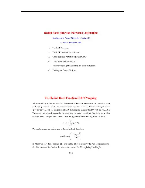
Computing the Output Weights Our equations for the weights are most conveniently written in matrix form by defining matrices with components (Wkj = wkj, (Φpj = φj(xp, and (Tpk = {tkp}. This gives Φ T ΦW T − T = 0 and the formal solution for the weights is ( W T = Φ †T in which we have the standard pseudo inverse of Φ Φ † ≡ (Φ T Φ −1 Φ T which can be seen to have the property Φ †Φ = I. We see that the network weights can be computed by fast linear matrix inversion techniques. In practice we tend to use singular value decomposition (SVD to avoid possible ill-conditioning of Φ , i.e. ΦTΦ being singular or near singular. L13-11Overview and Reading 1. 2. 3. 4. 5. We began by defining Radial Basis Function (RBF mappings and the corresponding network architecture. Then we considered the computational power of RBF networks. We then saw how the two layers of network weights were rather different and different techniques were appropriate for training each of them. We first looked at several unsupervised techniques for carrying out the first stage, namely optimizing the basis functions. We then saw how the second stage, determining the output weights, could be performed by fast linear matrix inversion techniques. Reading 1. 2. Bishop: Sections 5.2, 5.3, 5.9, 5.10, 3.4 Haykin: Sections 5.4, 5.9, 5.10, 5.13 L13-12。


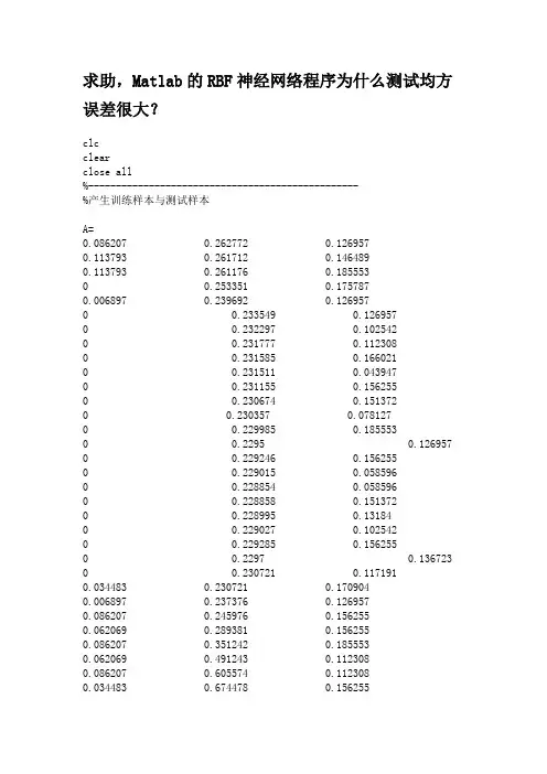
求助,Matlab的RBF神经网络程序为什么测试均方误差很大?clcclearclose all%-------------------------------------------------%产生训练样本与测试样本A=0.086207 0.262772 0.1269570.113793 0.261712 0.1464890.113793 0.261176 0.1855530 0.253351 0.1757870.006897 0.239692 0.1269570 0.233549 0.1269570 0.232297 0.1025420 0.231777 0.1123080 0.231585 0.1660210 0.231511 0.0439470 0.231155 0.1562550 0.230674 0.1513720 0.230357 0.0781270 0.229985 0.1855530 0.2295 0.126957 0 0.229246 0.1562550 0.229015 0.0585960 0.228854 0.0585960 0.228858 0.1513720 0.228995 0.131840 0.229027 0.1025420 0.229285 0.1562550 0.2297 0.136723 0 0.230721 0.1171910.034483 0.230721 0.1709040.006897 0.237376 0.1269570.086207 0.245976 0.1562550.062069 0.289381 0.1562550.086207 0.351242 0.1855530.062069 0.491243 0.1123080.086207 0.605574 0.1123080.034483 0.674478 0.1562550.062069 0.733842 0.1709040.196552 0.768613 0.1123080.086207 0.792452 0.1709040.034483 0.807965 0.1171910.086207 0.826889 0.131840.168966 0.844617 0.1660210.168966 0.859543 0.1367230.196552 0.879376 0.1367230.196552 0.894525 0.2246160.196552 0.911278 0.1464890.141379 0.922284 0.0585960.196552 0.927073 0.1367230.113793 0.930332 0.1464890.168966 0.932973 0.1464890.168966 0.938881 0.0634780.168966 0.94669 0.1025420.196552 0.952802 0.0976590 0.958737 0.1513720.006897 0.960443 0.1025420 0.96324 0.117191 0.113793 0.965827 0.0781270.034483 0.966464 0.2392650.113793 0.969583 0.1709040.086207 0.971601 0.1855530.141379 0.973354 0.131840.034483 0.974763 0.1367230.062069 0.975569 0.1171910.034483 0.976746 0.1367230.006897 0.977846 0.131840.062069 0.978429 0.1757870.086207 0.979458 0.1562550.062069 0.9806 0.1171910.006897 0.980925 0.1367230.141379 0.981492 0.1269570.086207 0.982099 0.1269570.113793 0.982412 0.1269570.141379 0.982897 0.1367230.141379 0.983022 0.1660210.141379 0.983042 0.1269570.168966 0.982819 0.1025420.113793 0.98267 0.1123080.034483 0.982283 0.1269570.062069 0.981973 0.1269570.034483 0.981375 0.1269570.034483 0.98087 0.097659 0.062069 0.980189 0.1367230.006897 0.979309 0.0927760.062069 0.97864 0.156255 0.034483 0.978171 0.1123080.086207 0.976915 0.1513720.034483 0.97639 0.092776 0.141379 0.974982 0.1367230.113793 0.97389 0.117191 0.141379 0.972857 0.1269570.006897 0.971918 0.1367230.034483 0.971257 0.1855530.034483 0.970788 0.1464890.141379 0.946456 0.1562550.141379 0.946006 0.1123080.196552 0.945368 0.1513720.196552 0.944625 0.1367230.168966 0.944014 00.168966 0.94322 00.168966 0.942578 00.086207 0.942183 0.1367230.168966 0.941189 0.6152530.168966 0.940438 00.113793 0.939679 0.2783290.168966 0.93903 00.113793 0.938545 0.7861570.141379 0.938212 00.113793 0.937371 0.8398690.141379 0.936737 0.1025420.196552 0.936103 00.141379 0.935489 00.196552 0.935199 00.168966 0.934507 0.1464890.168966 0.934213 0.2099670.168966 0.933709 0.1562550.168966 0.933075 0.1171910.168966 0.932586 0.0976590.196552 0.932183 0.0927760.196552 0.931936 0.1513720.141379 0.931326 0.131840.168966 0.931087 0.0781270.196552 0.92881 0.2246160.086207 0.928482 0.1660210.141379 0.927965 0.1123080.113793 0.927402 0.13184 0.113793 0.926866 0.13184 0.141379 0.926568 0.126957 0.141379 0.926392 0.097659 0.196552 0.926079 0.112308 0.141379 0.923708 0.097659 0.141379 0.923188 0.146489 0.113793 0.922887 0.097659 0.168966 0.922503 0.126957 0.141379 0.922053 0.102542 0.086207 0.921791 0.136723 0.086207 0.921463 0.151372 0.062069 0.921247 0.117191 0.086207 0.920946 0.078127 0.062069 0.920747 0.126957 0.113793 0.920484 0.136723 0.141379 0.920359 0.078127 0.034483 0.920121 0.063478 0.113793 0.918869 0.200201 0.062069 0.918626 0.327158 0.086207 0.918477 0.156255 0.141379 0.918254 0.327158 0.034483 0.918078 0.117191 0.034483 0.917879 0.078127 0.086207 0.917714 0.146489 0.006897 0.917589 0.063478 0.113793 0.917425 0.136723 0.086207 0.917167 0.136723 0.034483 0.917006 0.136723 0.062069 0.916232 0.073244 0.086207 0.916118 0.200201 0.113793 0.916056 0.092776 0.062069 0.915922 0.126957 0.086207 0.915762 0.058596 0.113793 0.915696 0.126957 0.168966 0.914048 0.185553 0.113793 0.913199 0.117191 0.113793 0.912487 0.185553 0.086207 0.912014 0.009766 0.168966 0.911642 0.078127 0.034483 0.911087 0.166021 0.168966 0.910637 0.200201 0.113793 0.910472 0.166021 0.196552 0.910324 0.1367230.141379 0.90978 0.131840.113793 0.907644 0.1660210.224138 0.907569 0.1464890.196552 0.907468 0.1464890.196552 0.907444 0.1367230.196552 0.907338 0.1171910.168966 0.907237 0.1269570.196552 0.907202 0.2050840.196552 0.907123 0.1269570.196552 0.907045 0.0781270.168966 0.906767 0.1660210.196552 0.906724 0.1513720.196552 0.906716 0.1123080.141379 0.906615 0.1513720.168966 0.906509 0.1855530.196552 0.906458 0.1562550.196552 0.906043 0.1123080.168966 0.905938 0.1709040.168966 0.905691 0.131840.168966 0.905394 0.126957; %训练样本,共三百组A=A';A1=A(1,:);A2=A(2,:);A3=A(3,:);B=3.1:.0458:16.8; %训练目标C=0.168966 0.905394 0.1269570.168966 0.905277 0.1025420.196552 0.905155 0.1367230.168966 0.905171 0.131840.141379 0.90519 0.1464890.141379 0.905194 0.048830.196552 0.905198 0.1171910.141379 0.905167 0.1269570.113793 0.905163 0.1123080.168966 0.905155 0.1123080.168966 0.905124 0.1513720.196552 0.905065 0.1171910.168966 0.905069 0.1367230.196552 0.905026 0.2002010.141379 0.905011 0.0781270.113793 0.904971 0.1709040.196552 0.904905 0.146489 0.141379 0.904881 0.151372 0.113793 0.904838 0.146489 0.168966 0.904799 0.156255 0.141379 0.904748 0.058596 0.168966 0.904717 0.112308 0.196552 0.904635 0.102542 0.141379 0.904627 0.126957 0.086207 0.904568 0.097659 0.196552 0.904545 0.097659 0.196552 0.904431 0.136723 0.196552 0.90442 0.117191 0.141379 0.904381 0.117191 0.168966 0.904353 0.136723 0.141379 0.904326 0.156255 0.168966 0.904259 0.13184 0.168966 0.904228 0.151372 0.168966 0.904224 0.063478 0.141379 0.904204 0.112308 0.141379 0.904212 0.126957 0.168966 0.904177 0.151372 0.141379 0.904146 0.151372 0.086207 0.90413 0.151372 0.141379 0.904099 0.078127 0.113793 0.904099 0.126957 0.086207 0.904079 0.146489 0.141379 0.904044 0.112308 0.168966 0.904025 0.092776 0.141379 0.903989 0.073244 0.113793 0.903985 0.092776 0.196552 0.90397 0.112308 0.196552 0.903954 0.097659 0.141379 0.903923 0.170904 0.113793 0.903888 0.112308 0.141379 0.903856 0.097659 0.168966 0.903817 0.13184 0.141379 0.903817 0.102542 0.141379 0.90379 0.073244 0.141379 0.903778 0.13184 0.141379 0.903762 0.073244 0.113793 0.903755 0.136723 0.062069 0.903719 0.175787 0.168966 0.903708 0.1513720.141379 0.903708 0.1123080.168966 0.903657 0.1855530.113793 0.903653 0.1171910.113793 0.903637 0.1367230.168966 0.90361 0.1709040.168966 0.903575 0.1269570.141379 0.903551 0.1025420.141379 0.903532 0.1367230.141379 0.903512 0.1367230.141379 0.903481 0.1513720.141379 0.903473 0.1269570.113793 0.903434 0.1367230.141379 0.903457 0.1171910.168966 0.903473 0.1757870.141379 0.903418 0.1171910.168966 0.903406 0.1562550.086207 0.903383 0.1562550.141379 0.903363 0.1464890.141379 0.903359 0.1367230.141379 0.903328 0.1123080.141379 0.903297 0.131840.141379 0.90325 0.1464890.168966 0.902917 0.1269570.168966 0.902851 0.131840.113793 0.902816 0.1855530.141379 0.902816 0.0732440.141379 0.902792 0.0781270.086207 0.902792 0.1464890.141379 0.902745 0.1660210.168966 0.902675 0.1171910.141379 0.902632 0.1562550.086207 0.902612 0.1367230.113793 0.902612 0.126957;%测试样本,共一百组C=C';C1=C(1,:);C2=C(2,:);C3=C(3,:);D=3.1:.1383:16.8; %测试目标%--------------------------------------------------%归一化[PN1,mina1,maxa1,TN,minb,maxb] = premnmx(A1,B);[PN2,mina2,maxa2,TN,minb,maxb] = premnmx(A2,B);[PN3,mina3,maxa3,TN,minb,maxb] = premnmx(A3,B);PN4 = tramnmx(C1,mina1,maxa1);PN5 = tramnmx(C2,mina2,maxa2);PN6 = tramnmx(C3,mina3,maxa3);TN2 = tramnmx(D,minb,maxb);A=[PN1;PN2;PN3];C=[PN4;PN5;PN6];%---------------------------------------------------% 训练switch 2case 1spread = 0.2;net = newrbe(A,TN,spread);case 2goal =0;spread =0.2;MN = size(A,2);DF = 25;net = newrb(A,TN,goal,spread,MN,DF);case 3spread = 0.2;net = newgrnn(A,TN,spread);end%--------------------------------------------------% 测试YN1 = sim(net,A); % 训练样本实际输出YN2 = sim(net,C); % 测试样本实际输出MSE1 = mean((TN-YN1).^2) % 训练均方误差MSE2 = mean((TN2-YN2).^2) % 测试均方误差%--------------------------------------------------% 反归一化Y2 = postmnmx(YN2,minb,maxb);%--------------------------------------------------% 结果作图plot(1:length(D),D,'r:',1:length(Y2),Y2,'b-');clear; >> xdata=xlsread('2011.xls'); >> x1=xdata(1:12,1:3); >> P1=x1'; >> T1 = [repmat([1;0;0],1,4),repmat([0;1;0],1,4),repmat([0;0;1],1,4)]; >> x2=xdata(13:44,1:3); >> P2=x2'; >> T2 = [repmat([1;0;0],1,9),repmat([0;1;0],1,10),repmat([0;0;1],1,13)]d=t123'; %ÇóתÖÃdp=[0.3 30000 0.001];B = int8(d);sizeofp=size(91);sizeft=size(1);[pn,meanp,stdp,tn,meant,stdt]=prestd(91,1);[ptrans,transMat]=prepca(pn,0.001);iitr1=6:3:1;iitr2=[9:3:1 9:3:1 6:3:1 6:3:1 4:3:1];P1=tranbr(:iitr1)P2=tranbr(:iitr2)。

RBF神经网络:原理详解和MATLAB实现——2020年2月2日目录RBF神经网络:原理详解和MATLAB实现 (1)一、径向基函数RBF (2)定义(Radial basis function——一种距离) (2)如何理解径向基函数与神经网络? (2)应用 (3)二、RBF神经网络的基本思想(从函数到函数的映射) (3)三、RBF神经网络模型 (3)(一)RBF神经网络神经元结构 (3)(二)高斯核函数 (6)四、基于高斯核的RBF神经网络拓扑结构 (7)五、RBF网络的学习算法 (9)(一)算法需要求解的参数 (9)0.确定输入向量 (9)1.径向基函数的中心(隐含层中心点) (9)2.方差(sigma) (10)3.初始化隐含层至输出层的连接权值 (10)4.初始化宽度向量 (12)(二)计算隐含层第j 个神经元的输出值zj (12)(三)计算输出层神经元的输出 (13)(四)权重参数的迭代计算 (13)六、RBF神经网络算法的MATLAB实现 (14)七、RBF神经网络学习算法的范例 (15)(一)简例 (15)(二)预测汽油辛烷值 (15)八、参考资料 (19)一、径向基函数RBF定义(Radial basis function——一种距离)径向基函数是一个取值仅仅依赖于离原点距离的实值函数,也就是Φ(x)=Φ(‖x‖),或者还可以是到任意一点c的距离,c点称为中心点,也就是Φ(x,c)=Φ(‖x-c‖)。
任意一个满足Φ(x)=Φ(‖x‖)特性的函数Φ都叫做径向基函数。
标准的一般使用欧氏距离(也叫做欧式径向基函数),尽管其他距离函数也是可以的。
在神经网络结构中,可以作为全连接层和ReLU层的主要函数。
如何理解径向基函数与神经网络?一些径向函数代表性的用到近似给定的函数,这种近似可以被解释成一个简单的神经网络。
径向基函数在支持向量机中也被用做核函数。
常见的径向基函数有:高斯函数,二次函数,逆二次函数等。