AMESim 01_AME_TH2_V4.3_thermal cn
- 格式:pdf
- 大小:809.62 KB
- 文档页数:30

史上最全的AMESim-Matlab 联合仿真设置步骤(集大成者,图文并茂)中国矿业大学机电学院 haierdhg目前,文库及网上流行的AMESim-Matlab 联合仿真步骤基本不能用,经过几天的研究,终于找到了解决方案。
本文论述了联合仿真的设置步骤、仿真时应注意的事项,以及有用的参考资料,敬请大家分享。
一、版本为AMESim8.0,Matlab2011b,VC++6.0二、安装步骤个人认为以上三个软件,没有安装顺序,但还是建议先安装VC++1.将VC++中的"vcvar32.bat"文件从Microsoft Visual C++目录(通常是.\Microsoft Visual Studio\VC98\Bin中)拷贝至AMESim目录下(我的是C:\AMESim\v800)。
(如果先安装的VC,后安装的AMESim,则在AMESim安装时,自动会拷贝该文件)2.环境变量确认:(这里网上的教程大多是错的!环境变量分为用户变量和系统变量,网上教程大多没说清楚)1)选择“控制面板-系统”或者在“我的电脑”图标上点右键,选择“属性”;2)在弹出的“系统属性”窗口中选择“高级”页,选择“环境变量”;3)用户变量中添加HOME C:\ (我将AMESim Matlab装在了C盘,自己根据情况修改) MATLAB C:\MATLAB\R2011bPath D:\Program Files\Microsoft Visual Studio\Common\Tools\WinNT;D:\Program Files\Microsoft VisualStudio\Common\MSDev98\Bin;D:\Program Files\Microsoft Visual Studio\Common\Tools;D:\Program Files\Microsoft Visual Studio\VC98\bin4)在系统变量中添加AME C:\AMESim\v800 (这个一般都有的,不需要自己添加);Path D:\Program Files\Microsoft Visual Studio;C:\AMESim\v800;C:\AMESim\v800\win32;C:\AMESim\v800\sys\mingw32\bin;C:\AMESim\v800\sys\mpich\mpd\bin;C:\AMESim\v800\sys\cgns;%SystemRoot%\system32;%SystemRoot%;%SystemRoot%\System32\Wbem;C:\MATLAB\R2011b\bin\win32;C:\WINDOWS\system32;C:\WINNT (该处很重要一定要添加,而且一定要包含C:\WINDOWS\system32,不然会有引起很多错误)3.确认是否在AMESim中选择VC作为编译器。
AMESIM 中文教程-第4章高级实例本章你将:• 搭建更复杂的系统• 稳定化运行• See aliasing with data sampling • 使用动态块• 使用旋转机械块4.1 1• 显示系统的状态变量• 用稳定化运行发现初始值• 在图形比较使用保存和装载数据• 给曲线添加文本4.1.1状态计数功能使你能看到仿真中显示的状态变量(外部的或隐含的或约束的),该功能作为快速观察状态变量标题的方式也是非常有用的。
在时间阶跃步序列中,积分过程要持续进行到终点。
在每一个阶跃步,都使用这个重复过程来确定状态变量在新时刻的值。
这一重复过程必须成功地收敛于阶跃过程;此外,每一步之后,都要基于运行参数对话框指定的允许误差进行误差测试。
在某特殊步,一些状态变量可能很容易满足收敛和误差测试,而其它变量则勉强通过测试。
AMESim 记录下满足测试有极大困难的状态变量,在运行模式,通过点击状态计数按钮,将出现状态计数对话框,它会摘述一些信息,这些信息对于确定慢仿真过程非常有用。
继续上一章的实例,再下载已经创建的QuarterCar.ame 文件。
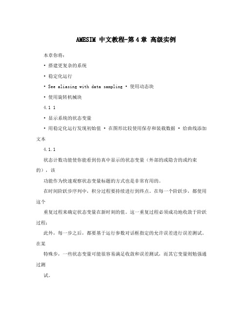
为确保该实例所描述的过程对你的系统有意义,在参数模式下请确认如下数值已被设置:子模型草图上的数量(如果有)标题数值 Body_Mass/MAS002 1 body velocity 0.0body displacement 0.0SPR000A 2 2 spring force with both 0.0displacements zero Wheel_Mass/MAS002 3 wheel velocity 0.0wheel displacement 0.0 SPR000A 4 spring force with both 0.0displacements zero进入运行模式进行仿真,有5个状态变量,请点击状态计数按钮产生如图4.2所示对话框:Figure 4.2本例中,使运行速度变较的很可能是子模型为MAS002 (车轮质量)的状态变量(wheel velocity),如果仿真缓慢,你可以点击更新(Update)按钮或自动更新对话框。

第一章引言本章将介绍AMESim 家族产品和AMESim 4.2 的新特征。
AMESim 是什么? AMESim 怎么用? 如何使用文件组?在线帮助的组织结构。
AMESim 4 软件包。
AMESim 4.2 的新特征1.1 AMESim 是什么?AMESim表示工程系统仿真高级建模环境(A dvanced M odeling E nvironment for performing Sim ulations of engineering systems). 基于直接图形接口,在整个仿真过程中系统可以显示在环境中。
AMESim 使用图标符号代表各种系统的元件,这些图标符号要么是国际标准组织如工程领域的ISO为液压元部件确定的标准符号,或为控制系统确定的方块图符号,或者当不存在这样的标准符号时可以为该系统给出一个容易接受的非标准图形特征。
. Figure 1.1: AMESim 中使用符号Figure 1.1 所示为使用标准液压,机械和控制符号表达的一个工程系统。
Figure 1.2所示为使用了非标准图形特征的汽车制动系统。
Figure 1.2: 汽车制动系统的符号1.2 如何使用AMESim?使用AMESim 你可以通过在绘图区添加符号或图标搭建工程系统草图,搭建完草图后,可按如步骤进行系统仿真:• 图标元件的数学描述• 设定元件的特征• 初始化仿真运行• 绘图显示系统运行状况Figure 1.3 所示为从HCD符号构建的一个三柱塞径向液压泵详细模型。
箭头用来表示液流方向。
Figure 1.3: 从HCD符号构建的一个三柱塞径向液压泵大多数自动化系统都可按上述步骤执行,在每一步都可以看到系统草图。
接口现在的联系是为了提供软件间的接口使它们能够联合工作,以便你能够获得每个软件的最佳特征。
标准AMESim软件包提供了与MATLAB.的借口。
这使你有权使用控制器设计,优化工具和功率谱分析等。
还有其它一些接口可用,AMESim 最新接口信息请参见1.6.6节接口。
Electric Motors and Drives LibraryRev 9 – November 2009Copyright © LMS IMAGINE S.A. 1995-2010AMESim® is the registered trademark of LMS IMAGINE S.A.AMESet® is the registered trademark of LMS IMAGINE S.A.AMERun® is the registered trademark of LMS IMAGINE S.A.AMECustom® is the registered trademark of LMS IMAGINE S.A.LMS b is a registered trademark of LMS International N.V.LMS b Motion is a registered trademark of LMS International N.V. ADAMS® is a registered United States trademark of MSC.Software Corporation. MATLAB and SIMULINK are registered trademarks of the Math Works, Inc. Modelica is a registered trademark of the Modelica Association.UNIX is a registered trademark in the United States and other countries exclusively licensed by X / Open Company Ltd.Python is a registered trademark of the Python Software Foundation.Windows is the registered trademark of the Microsoft Corporation.All other product names are trademarks or registered trademarks of their respective companies.TABLE OF CONTENTS1.Introduction (1)2.Generalities (2)2.1. Scope of the library (2)2.2. Electric motors and icons (2)2.2.1. Motor description (2)2.2.2. Motor icons (3)2.3. Notations and conventions (3)2.4. Basic sketch: a first electric motor model (5)2.5. Library structure and content (6)2.6. Instructions for the demonstration usage (8)ing the EMD library (8)3.1. Direct current motor (8)3.1.1. Permanent excitation (8)3.1.2. External excitation (10)3.1.3. Brushless DC motor (13)3.2. AC Machine (16)3.2.1. Synchronous motor (16)3.2.2. Induction machine (22)3.3. Battery and alternator (31)3.4. Tabulated motor (34)3.5. Control elements (37)3.5.1. Sensors (37)3.5.2. Park (dq0) transformation (38)4.Annexes (39)4.1. Glossary (39)4.2. Squirrel cage induction machine parameterization (41)References (42)Using theElectric Motors & Drives Library(EMD)1. IntroductionNowadays, numerous equipments are powered with electrical actuator. In order to get an accurate evaluation of energy needs as well as to evaluate the impact of the actuators dynamic on the whole system, it is important to represent the precise behavior of electric motors and drives.The “Electric Motors and Drives” (EMD) library aims at providing a set of high level models to reach this objective. It covers the main needs regarding electromechanical conversion simulation.The sub-models in the EMD library represent the commonly used electric machines:- Direct Current machine: permanent or separated excitation- Synchronous machine: round or salient rotor, with or without dampers- Induction machine: squirrel cage or wound rotor- Brushless Permanent Magnet machine- Tabulated machine (quasi-static)Moreover, control elements are added in order to build advanced motor control:sensors- Currentsensors- Voltagesensors- Power- Direct and reverse Park/Concordia transformFinally, generators are also available:- Tabulated alternator with rectifier (quasi-static)- BatteriesThis manual presents the EMD library. The first part of the document gives general assumptions relevant to electric machine modeling. Conventions and notations are then introduced associated with a brief explanation about electric motors structure and the icons appearance. It is concluded by a first sketch demonstrating the use of an electric motor in simulation.The second part goes into deeper detail with the EMD content in providing basic examples for various EMD elements.In this manual, it is assumed that the reader is familiar with the use of the b AMESim environment. Moreover, knowledge of additional libraries is required, it is therefore recommended to read the following manual for more information:- Mechanical Library manual- Electrical Basic Library manual- Electrical Static Conversion Library manual- Thermal Library manual2. Generalities2.1. Scope of the libraryThe Electric Motors and Drives library (EMD), aims at modeling any electromechanical conversion chain, providing the engineers with a set of high level models for commonly used electric motors.In this purpose, it answers complex mechatronic issues in dealing with electrical as well as mechanical and thermal phenomena.The electric motors and drives components are made for system simulation, representing the energetic interactions with their environment; the details of electric motor geometry are therefore not taken into account. For example, the teeth variation torque or the saturation of magnetic material in the motor are then not represented.Moreover, it is assumed that the electric motors do not suffer construction default so that the windings are mechanically well balanced and electrically equilibrated.The user must note that electric machines are fully reversible devices. They can produce mechanical energy from electrical energy and vice-versa. Unless specified, every machine can therefore work asa motor or as a generator.2.2. Electric motors and iconsThe present document does not aim at giving a complete course about electric motors; the user is therefore strongly advised to refer to [Sen96] to get more information about machines.However, to better understand this document’s explanations, a brief introduction of basic notions about electric motors will help.2.2.1. Motor descriptionAn electric motor is represented in Figure 1 and a possible construction proposed with a hypothetical cross section:Figure 1: Electric motor compositionMechanicalAn electric motor is composed of two major mechanical part exchanging energy by the means of magnetic fields:-The rotor; having a rotational movement and transmitting the produced torque to the mechanical load.-The stator; static part of the actuator, linked to the system base.Electrical and magneticElectric motors embed two magnetic field sources. One is linked to the stator and the other to the rotor. These magnetic sources can be:-Electric windings: made of copper or aluminum (good electrical conductors). There is at least one of these in every machine.- A set of magnet.ThermalEvery electric motor is composed of iron material on both stator and rotor parts to increase the magnetic flux and the global efficiency of the electromechanical conversion, and electric conductor materials in the windings. These materials have specific properties depending on the environment temperature.Besides, the current flowing in the electric conductors produces a heat flow exchanged with the environment.2.2.2. Motor iconsThe machine icons represent this structure of electric motor. An example is given in Figure 2:Figure 2: Example of electric motor icon in EMDThe mechanical parts (stator and rotor) are identified by circles (external and internal) according to the standard [ISO] representation. Both parts mechanical interactions are managed with rotational mechanical ports.The electrical windings can be connected to a circuit with electrical ports, whose number depends on the machine technology. A three phase winding machine has three electrical ports to connect while a single phase winding has two. When a motor contains magnets, an additional symbol is displayed on the icon (Figure 3):Figure 3: Magnet SymbolThe thermal quantities are exchanged through thermal ports, allowing to build an electro-thermal representation of the motor.2.3. Notations and conventionsElectrical conventions: dipolesThe passive and active sign conventions for dipoles are represented in Figure 4:Passive convention Active ConventionFigure 4: Electrical convention for current and voltageBoth conventions are used in EMD. For example, electric machine phases are considered to take power from the circuit and use the passive sign convention, indicated on the icons with a white dot. On the contrary, generators phases are considered to give power to the circuit and use the active sign convention, indicated on the icon with a dark dot. Examples of icons for both cases are given in Figure 5:Figure 5: EMD icons with passive (white dot) and active (dark dot)sign conventionFor both the machine and the battery, the power exchanged with the circuit can be positive or negative since these devices are reversible. However, the dot on the icon indicates the type of convention used and explicit the direction of the voltage and current quantities:- Submodels using the passive sign convention have input voltage and input currentvariables as represented in Figure 4. The product of these quantities is a power,positive if energy is going into the model.- Submodels using the active sign convention have output voltage and output currentvariables as represented in Figure 4. The product of these quantities is a power,positive if energy is going out of the model.Electrical conventions: three phase windingsThree phase machines only have three electrical ports since the windings are connected in a star or delta connection. The electrical ports are associated on icons with the symbols I , II and III .The equivalent windings in the three phase machine are called A , B and C .The winding connection, the current and voltage direction and relation with the electrical ports are summarized in Figure 6:Star (or Y) Connection Delta (or Triangle) ConnectionFigure 6: Winding connection and electrical convention for threephase machinesThe windings individually therefore always use the passive sign convention.Electrical conventions: electrical angleThe phase A is the reference for the stator. The phase A or the field phase is the reference for the rotor. The electrical angle is then the angle between the stator and the rotor references.Moreover, the windings order in the machine is A, B, C and they have an electrical phase lag of 32πrad with each others. If we set a constant magnetic field in the machine rotor for example and put it in motion so that the electrical angle rises, a back electromotive force will be created in thestator phases. The rotation will indeed create a flux linkage variation from the stator phase point of view. Then the back electromotive force created in the A phase when the electrical angle is 0 rad will be the same as the back electromotive force created in the B phase when the electrical angle is 32πrad. The electrical angle and the winding position for the stator can be summed up in Figure 7:Figure 7: Electrical angle definitionMechanical conventionThe mechanical ports for electric motors exchange energy that is positive when going into the machine. Therefore, when a torque produced by an electric motor is applied to a mechanical load and has the same sign as the rotary velocity quantity at the machine port, the machine is actually braking.On the opposite, if the torque and rotary velocity quantities have opposite signs at the machine port, the machine works as a motor.2.4. Basic sketch: a first electric motor modelTo illustrate the library features better, we present a first model with an electric motor connection.A simple but complete example we can build is a basic DC motor with permanent magnet excitation. It is represented in Figure 8:Figure 8: Basic sketch for an electric motorIt is important to note that the EMD machine submodels only represent the machine circuits electrical dynamics in the transformation of electrical energy into mechanical energy. The mechanical dynamics must be modeled with other components and the torque the machine computes only is the electromagnetic torque. For example, the resistive torque from the load, frictions in the load or in themachine and inertia of the load and machine can be represented with the additional submodels RL01, TORQC and UD00.Similarly, the thermal diffusion in the machine and its environment could have been represented with thermal capacitances and resistances from the TH library in addition to the machine submodel. Here we only use a constant temperature source.On the model in Figure 8, the motor is also connected to the null velocity source submodel W000. It represents the connection of the machine stator to a fixed frame. Indeed, even if in most cases the stator does not move, it can be linked to any other mechanical body.Finally, the power supply of electric motor is represented using a controlled voltage source EBVS01 from the Electrical Basics (EB) library with a constant signal source CONS0.2.5. Library structure and contentThe structure of the EMD library is shown in Figure 9. The submodels are sorted into subfolders:Figure 9: EMD library structureThe EMD library is structured according to the standard classification of Electric Motors.The All repository contains a complete list of the EMD components (Figure 10):Figure 10: EMD library contentThe Synchronous Machines repository contains the synchronous motors and brushless motors components (Figure 11):Figure 11: Synchronous machine iconsThese machine models can represent various behaviors depending on their geometry (round or salient rotor poles), structure (rotor with or without dampers), stator connection (star or delta), or excitation type (permanent or external).To select some of these features, enumeration parameters are available. However, for others it is the submodel choice that enables the selection of these features. Table 1 gives a description of the submodels and the specific features associated with them.Icon Name MotordescriptionEMDSMPE01 Synchronous motor with permanent excitationno dampersEMDSMPED01 Synchronous motor with permanent excitation with dampersEMDSMES01 Synchronous machine with separatedexcitation no dampersEMDSMSED01Synchronous machine with separated excitation with dampers EMDBLM01Star connected brushless machine (DC or synchronous) EMDBLM02 Delta connected brushless machine (DC orsynchronous)Table 1: Synchronous machines submodels descriptionThe Induction Machines repository contains the induction machine components: squirrel cage and wound rotor machines (Figure 12):Figure 12: Induction machine iconsThe Direct Current Machines repository contains the DC machine components: permanent and external excitation (Figure 13):Figure 13: Direct current machine iconsThe Generators repository contains the generators components: batteries and tabulated alternator (Figure 14):Figure 14: Generator iconsFinally the Control Elements, Sensors and Line repositories contain components to design control systems and simplify sketches with three phase electric line merging (Table 2):Control Elements Sensors LineTable 2: Other EMD components2.6. Instructions for the demonstration usageThis manual explains how to deal with the Electric Motors and Drives library. Numerous examples are presented and the parameters and used submodels name given to make it possible to build the example model. However, it is possible to get a local copy of the demonstration in the help menu to easily get started with a new application (Figure 15):Figure 15: Get AMESim demo Item3. Using the EMD library3.1. Direct current motorEven though the Direct Current Motor (DC Motor) is not the most widely used machine in the industry, it represents a satisfying first level approximation for numerous system simulations. Indeed, its behavior is simple with little or no need for power electronic in its control.3.1.1. Permanent excitationThe permanent magnet brushed DC motor covers a wide part of small device electric motor needs (toys, hand tool, small actuator) since it is easy to supply (a simple battery suffices), moreover it can be cheap to produce.The following example introduces the use of a Permanent Excitation DC Motor in plotting the set of characteristic curves to be used for motor sizing.The first step is to build the sketch on Figure 16 (Permanent magnet DC motor characteristic01_PermanentExcitationDCMotor.ame):Figure 16: Basic simulation for a permanent magnet DC motorThe second step is to set the right submodels and their appropriate parameters values, found on supplier’s data sheet for example. They are summed up in Table 3:Icon Name Parameter Value UnitTHTS1-1 Temperature at port 1 25 degC EMDDCPE01-1Armature winding input current #3 A excitation type Permanen t magnetNullReference temperature 25 degCarmature winding resistance at reference temperature 16 Ohmcorrective coefficient on armature winding resistance 0.004 1/K armature winding inductance 0.00414 H Back EMF and torque constant at reference temperature 0.214 V*s/rad Corrective coefficient on back emf and torque constant -0.002 1/KRL01-1Moment of inertia 1.23e-5 Kgm**2 Coefficient of viscous friction 2.5e-6 Nm/(rev/min) Coulomb friction torque 0.267 Nm Stiction torque 0.267 Nm SupplyvoltageCONS0 constant value 48 V Inputtorque UD00-1 number of stages 1 cyclic no time at which duty cycle starts 0 s output at start of stage 1 0.641output at end of stage 1 0duration of stage 1 50Table 3: Parameters for the model in Figure 16Now that the parameters have been set, switch to Simulation mode and run a simulation for 100 s, with a communication interval of 0.5 s. Let the tolerance at its default value (1e-5).Then, to plot the interesting quantities relevant to the motor characteristics, it is possible to use post-processing tools. Add the inertia torque at port 1 and shaft speed port 2 and motor winding input current and armature winding input voltage to the post processing window. From these 4 variables it is then possible to compute the motor mechanical power, electrical power and efficiency (see Figure17).Figure 17: Post processing variable computationWe can now with XY plots represent the motor speed, input current, mechanical power and efficiency as a function of the motor torque. These characteristic curves are displayed on Figure 18; they can also be obtained using the Analysis/load plot configuration menu and selecting the “01_PermanentExcitationDCMotor_.plt” file.Figure 18: DC motor characteristic curvesThese characteristic curves are very interesting to help selecting appropriate motors for a system sizing. Depending on the application, the choice can be made focusing on various criteria such as the maximum mechanical power or the global efficiency.To go further, it is possible with this example to observe the supply voltage level influence on the DC motor characteristics.3.1.2. External excitationAnother simple example is presented here featuring a DC motor with external excitation. Such machines are often used in application with higher power needs (above 5kW) and both speed and torque control requirements.This example studies the start of an inertia load. The model sketch is represented in Figure 19 (Separated excitation DC motor on inertia 02_IndependentExcitationDCMotor.ame):Figure 19: Independent excitation DC motorUsing the independent excitation DC motor, it is possible to control both torque and speed applied to the mechanical load.Indeed, in applying a variable voltage to the armature (rotor) and field (stator) winding, it is possible to control the speed and the electromagnetic torque. In this basic example however, we only vary the field voltage.The submodel names and parameters to use for the model in Figure 19 are summed up in Table 4. In addition to the winding inductances, the machine is characterized with winding resistances and flux linkage coefficient (“back EMF and torque reduced constant” parameter ) depending on the temperature. Refer to Material properties for more information about the temperature corrective coefficients values.Icon Name Parameter Value UnitTHTS1-1 Temperature at port 1 25 degC EMDDCSE01-1Armature winding input current #0 A Field winding input current #0 A excitation type Permanen t magnetNullreference temperature 25 degCarmature winding resistance at reference temperature 0.6 Ohmcorrective coefficient on armature winding resistance 0.004 1/K armature winding inductance 0.012 H field winding resistance at reference temperature 240 Ohm corrective coefficient on field winding resistance 0.004 1/K field winding inductance 120 H Back EMF and torque constant at reference temperature 0.18 V*s/rad Corrective coefficient on back emf and torque constant 0 1/KRL01-1Moment of inertia 0.5 Kgm**2 Coefficient of viscous friction 0.002 Nm/(rev/min) Coulomb friction torque 0 Nm Striction torque 0 Nm Supplyvoltage CONS0-1constant value 240 V UD00-1number of stages 3Excitation supply cyclic no time at which duty cycle starts 0 soutput at start of stage 1 100output at end of stage 1 100duration of stage 1 20 soutput at start of stage 2 100output at end of stage 2 200duration of stage 2 10 soutput at start of stage 3 200output at end of stage 3 200duration of stage 3 1e6 sResistive torque CONS0-2constant value 10 Nm Table 4: Parameters for the model in Figure 19Now that the parameters have been set, switch to Simulation mode and run a simulation for 50 s, with a communication interval of 0.01 s. Let the tolerance at its default value (1e-5).It is interesting to compare the inertia speed with the field voltage. Plot the two variables on a same graph to emphasize their correlation (Figure 20), or get them loading the plot configuration file02_IndependentExcitationDCMotor_.plt:Figure 20: Field voltage and inertia speedThe armature current is displayed in Figure 21:Figure 21: Armature current while starting of externaly excited DCmotorThe motor rotary velocity varies over time, therefore the machine back electromotive force (bemf) in the armature winding varies too. Even though the armature voltage is constant, the armature current evolves in response to the bemf variation. The current peak at start is also explained by this remark since at start the bemf is null.3.1.3. Brushless DC motorThe Brushless DC motor (also known as BLDC or PMBLDC) is often used in application where a position or speed regulation is needed, but its high efficiency and power/weight ratio makes its usage even more common.The following example presents a model for the various elements of an electromechanical chain to get started with the use of a BLDC motor: a power supply (DC), a power conversion system to command the motor (inverter with the commuter command signal generation), the motor and the mechanical load. The BLDC motor is self commutated, and the control features a constant (1 or -1) to select the rotation direction. It is represented on Figure 22 (Self commutated brushless DC motor 03_BLDC_self_commutated.ame):Figure 22: Full step control for BLDC motorThe BLDC machine stator winding used has a star connection. This feature can be set in selecting the appropriate submodels (EMDBLM01 for star connection, EMDBLM02 for delta connection), asdisplayed on Figure 23:Figure 23: Selection for internal windings connectionThe torque constant data file or expression is a function of the electrical angle. It represents thevariation of the field flux linkage in the stator with the A phase for a reference. For example, withTcoef = γ*cos(θe), the coupling between the field and the phase A is maximum when the electrical angle is null, with a bemf in phase A reaching its maximum.The machine command is known as full-step control, as the input voltage applied to the stator windings only takes 6 states (Figure 24). As the machine rotates, the input voltage will switch from one to another, creating a rotating magnetic flux.Figure 24: 6 positions for the stator input voltage and magnetic field The inverter commuters creating the motor input voltage switch states with the motor position evolution. The BLDC motor is then said to be self commutated. A position sensor is therefore needed for this control. It is an ideal sensor in this demonstration example, but industrial drives can embeds hall sensors to measure the rotor position.The full step command sequence produces currents with a specific shape displayed on Figure 25:Figure 25: Classic current shape full-step controlThe motor electromagnetic torque presents periodical variations that can create mechanical vibrations in the structure (displayed on Figure 26, it can be loaded from the plot configuration file03_BLDC_self_commutated_.plt). The full step control is thus known as a noisy control.Figure 26: Cogging torque with full-step control3.2. AC MachineThe Electric Motors and Drives library contains description for three phase machines. Such machines are built around three electrical windings in order to create a rotating magnetic field. Powering these machines can be achieved by two connection diagram: star or triangle.For synchronous and induction machine in EMD, this choice is made an enumeration parameter (Figure 27):Figure 27: Combo box for winding connection selection Similarly, synchronous and induction machine rotor geometry can be selected with an enumeration parameter. The poles can be round or salient (Figure 28):Figure 28: Rotor type selection3.2.1. Synchronous motorA synchronous machine (SM) is an electromagnetic actuator in the stator and rotor magnetic field rotates at the same speed, they are said to be synchronous.The EMD library contains two three phase synchronous machine: with external or permanent excitation3.2.1.1. External excitationMost alternators are external excitation synchronous machines. In this demonstration, a constant speed mechanical source (we assume a speed regulation by external means for example) powers a SM. The alternator output power is converted into DC power with a diode bridge rectifier, and a control loop regulates the output voltage applied on a resistive load.To control the DC output voltage, the SM field winding voltage is commanded. Indeed, the excitation field influences the alternator current production.The model sketch is displayed on Figure 29 (Synchronous generator on RC load voltage regulation 09_Voltage_regulation_synch.ame):Figure 29: Example of voltage regulation with an alternatorIn this example, the voltage reference to follow is various step objectives. Moreover, the load resistance is modified in the middle of the simulation to create a variation in the load current consumption.The model parameters for each sub-model are described in Table 5:Icon Name Parameter Value UnitTHTS1-1 Temperature at port 1 25 degC EMDSMSE01-1 Electrical angle #0 Rad Stator current on Park’s d axis #0 A Stator current on Park’s q axis #0 A Rotor typeRound - Winding connectionStar - Number of poles pairs1 - Reference temperature25 degC Stator winding reference at referencetemperature0.2 Ohm Corrective coefficient on stator windingresistance 0 1/K Stator cyclic inductance0.1 H Field winding resistance at referencetemperature0.2 Ohm Corrective coefficient on field windingresistance0 1/K Field winding inductance0.007 H Mutual inductance between stator and field0.005 HCONS0-1 Constant value 2000 - EBC01-1 Output voltage # 0 V capacitance 0.005 F UD00-2 VariableresistanceNumber of stages 2 - cyclic no - Time at which duty cycle starts 0 s Output at start of stage 1 4 - Output at end of stage 1 4 - Duration of stage 1 5 s Output at start of stage 2 6 - Output at end of stage 2 6 - Duration of stage 2 5 s PID001-1Integral part # 0 - Controller type PILimit output Yes。

Chapter 2: AMESim 工作空间章节描述::• AMESim用户接口• AMESim的四个工作模式• 一些诀窍和技巧2.1 AMESim用户接口AMESim 用户接口是基本工作区域,取决于工作模式,你可选择各种工具。
• 主窗口• 菜单条• 工具栏• 右击鼠标菜单• 各种库2.1.1 主窗口启动AMESim当启动AMESim时, 菜单窗口是空的。
Figure 2.23: AMESim主窗口标题栏最小化,恢复,关闭按钮你可以:• 要么打开一个空文本系统:• 下载一个已经存在的系统:当你下载一个已经存在的系统时,会出现一个浏览器以便指示你要打开系统的路径。
.Figure 2.24: 浏览器1. 选择你要打开的系统并点击打开项“Open”,2. 或者双击要打开的系统。
关闭AMESim当你关闭主窗口时,就自动退出了AMESim。
要关闭主窗口,按如下即可:• 点击关闭按忸(close),• 按Ctrl+Q键,• 在主菜单中选择文件菜单中退出键(File _ Quit),我们将描述AMESim W主接口的组成(请参见图表2.23)2.1.2 主菜单主菜单使你进入AMESim的主特征。
Figure 2.25: 主菜单注:通过菜单中已经给出的键盘快捷键还有其它一些特征,请参见键盘快捷键列表。
2.1.3 工具栏工具栏显示了对应于AMESim主特征的按钮。
你可以选择好多种工具栏:• 在所有模式下:• 文件操作工具栏• 模型操作工具栏• 注释工具栏• 瞬时分析工具栏•在运行模式下:• 后台处理工具栏• 线性分析工具栏要了解AMESim更多的工作模式,请见34页“AMESim的四个工作模式”。
文件操作工具栏要创建草图,请打开新系统。
要修改或完成已经存在的系统请打开它。
保存你创建系统。
模式操作工具栏Figure 2.26: 草图模式Figure 2.27: 子模型模式Figure 2.28: 参数模式Figure 2.29: 运行模式模式操作工具栏依你正在工作的模式而改变。

系统仿真AMESim软件使用说明目录1.AMESim是什么?2.AMESim 建模步骤?3.AMESim接口4.AMESim标准库5.AMESim软件包6.AMESim参数和变量观察7.AMESim建模(调用已有模型,讲解各元件及相互间联系)1.AMESim是什么?AMESim表示工程系统仿真高级建模环境(Advanced Modeling Environment for performing Simulations of engineering systems).基于直接图形接口,在整个仿真过程中草图系统可以显示在环境中。
AMESim 使用图标符号代表各种系统的元件,这些图标符号要么是国际标准组织(如工程领域的ISO为液压元部件)确定的标准符号、控制系统确定的方块图符号,或者当不存在这样的标准符号时可以为该系统给出一个容易接受的非标准图形特征。
Figure 1.1: AMESim中使用符号(标准液压,机械和控制符号表达的一个工程系统)Figure 1.2: 汽车制动系统的符号(非标准图形特征)2.如何使用AMESim?可按如步骤进行系统建模仿真:• sketch mode (草图模式)----从不同的应用库中选取现存的图形• submodel mode (子模型模式)----为每个图形选择子模型(即给定合适的数学模型假设)• parameter mode (参数设置模式)----每个图形模型设置特定的参数• simulation mode (仿真模式)----运行仿真并分析仿真结果大多数自动化系统都可按上述步骤执行,在每一步都可以看到系统草图。
3.接口与脚本you have the possibility of interfacing with Matlab/Simulink to test the Electronic Control Unit (ECU) of the complete gearbox and have the complete simulation platform for the conception of every kind of gearboxes3.1接口3.2 脚本4.标准库标准库提供了控制和机械图标,子模型允许你完成大量工程系统的动态仿真。
为方便模型交流,拷给同事直接能打开运行的方法最简单的方法为啥也不用管,只需记住模型所在文件夹数据文件所在文件夹,详细操作见help中Pack/Unpack facility(需将slave中的文件放在E:\systemmodel\XX_.slaves_dir\从名(如injector)_data\数据文件名)下面为个人试验总结方法:AMEsim有两种方法方便所需调用文件(如电磁阀的flux.data和force.data)的寻址1.将文件跟.ame模型放在同一个文件夹(这个应该是相对寻址)如模型在E:\systemmodel\XX.ame可将数据文件放在E:\systemmodel\data路径下,自己手动寻址一遍(或者直接输入data\文件名),只需将E:\systemmodel文件夹直接打包就可以在别人电脑上解压后直接运行。
、2.用绝对寻址方法如模型在E:\systemmodel\XX.ame需将数据文件放在E:\systemmodel\XX文件夹下如E:\systemmodel\XX\data\文件名这是只能手输入${circuit_name}/data/文件名即可PS:对于一些特殊的模型如master slave的DP系统master用的数据文件可直接按上述方法1或2即可而slave用的数据文件需将数据文件放在文件打开后生成的模型名_.slaves_dir文件夹下如demo中的高压共轨DP模型模型在E:\systemmodel\XX.ame用方法1:Slave用的数据文件应放在E:\systemmodel\XX_.slaves_dir\data\数据文件名(关掉模型后找不到该文件夹,再打开会重新生成)用方法2:Slave用的数据文件应放在E:\systemmodel\XX_.slaves_dir\slave名(如injector1)\data\数据文件名再手动输入${circuit_name}/data/文件名即可另外$AME指向安装目录X:\AMESim\V1000个人觉得方法1更好用个人愚见,如对您的使用带来方便,鄙人不胜荣幸,有更方便的方法,还请不吝赐教!BIT 王月强QQ:977508532。
Chapter 3: 入门本章你将作三个练习,使用AMESim主要功能搭建工程系统,分析它们的动态特性。
通常大约需要3~4小时,但因人而异差别较大。
而且,练习是可扩展的,在每一个练习的最后都有可供进一步研究的可选建议。
做完这些练习后,你因该能够使用标准AMESim元件和子模型进行简单的仿真。
我们建议你要立即或读完之后不久作这些练习。
3.1 启动AMESim使用Unix:请教系统管理员,请他给你演示如何设置工作环境以便进入。
要启动AMESim, i在合适的窗口,改变成你希望工作的路径,然后打印:AMESim使用Windows:按如下之一操作:•从菜单程序选择AMESim_ Imagine AMESim _通过启动按钮产生AMESim,或者:•双击桌面上的AMESim 图标,或者:•在MS DOS 命令窗打印AMESim。
你可以配置窗口,以便从Windows 资源管理器双击系统文件(.ame文件)就可以自动启动AMESim。
请参考安装注解中的设置程序。
图3.1显示的是AMESim a主显示器。
Figure 3.1: AMESim 主界面本显示器是空的,因没有打开或创建模型。
要搭建一个系统,必须创建一个新空模型。
然后才能在计算机上设计草图,存储系统。
Figure 3.2: 创建新的空模型3.2 创建新草图3.2.1 打开一个空系统要创建新草图,按如下之一即可:•点击打开空系统图标然后只有点击OK按钮才能得到如图3.2所示的窗口。
进行仿真的第一阶段就是搭建你要研究的系统,通过挑选并把各个元件放置在合适位置即可搭建系统。
进一步学习之前,我们要介绍一些AMESim工具栏的按钮,要想了解更多工具栏知识,请参考26页“工具栏”一节。
3.2.2 上(开)锁按钮上(开)锁按钮在模式操作工具栏里,用于上锁和开锁。
上开锁按钮是一个安全装置,放置你由于偶然因素改变系统,如果你不能修改系统,系统很可能处于锁定状态,当这个按钮处于上锁状态时,你不能修改系统草图。
amesim膨胀阀参数摘要:一、前言二、amesim膨胀阀简介1.定义与作用2.分类三、amesim膨胀阀参数设置1.参数类型2.参数意义与作用3.参数设置方法与技巧四、amesim膨胀阀参数对系统性能的影响1.参数对膨胀阀工作性能的影响2.参数对系统稳定性的影响3.参数对系统能效的影响五、总结正文:一、前言amesim膨胀阀作为制冷系统中的关键部件,对系统的性能、稳定性和能效具有重要的影响。
本文将详细介绍amesim膨胀阀的参数设置及其对系统性能的影响。
二、amesim膨胀阀简介amesim膨胀阀是一种用于调节制冷系统中制冷剂流量的装置,通过改变制冷剂流量的方法,维持系统运行在最佳状态。
1.定义与作用amesim膨胀阀主要作用是调节制冷剂的流量,以保证制冷系统在不同的运行条件下都能高效稳定地运行。
2.分类amesim膨胀阀根据结构、工作原理和控制方式的不同,可以分为多种类型。
三、amesim膨胀阀参数设置amesim膨胀阀参数设置是保证膨胀阀性能的关键,主要包括以下几个方面:1.参数类型amesim膨胀阀参数主要包括流量控制参数、温度控制参数、电磁阀控制参数等。
2.参数意义与作用流量控制参数用于设定膨胀阀的开启度,以控制制冷剂流量;温度控制参数用于设定膨胀阀的感温包位置,以实现自动调节;电磁阀控制参数用于设定电磁阀的开启和关闭,以控制膨胀阀的开启和关闭。
3.参数设置方法与技巧amesim膨胀阀参数设置需要根据制冷系统的具体工况进行调整,以保证膨胀阀在最佳状态下工作。
四、amesim膨胀阀参数对系统性能的影响amesim膨胀阀参数设置对制冷系统的性能、稳定性和能效具有重要的影响。
1.参数对膨胀阀工作性能的影响合理的参数设置可以保证膨胀阀在各种工况下都能正常工作,从而保证制冷系统的稳定运行。
2.参数对系统稳定性的影响amesim膨胀阀参数设置对系统稳定性的影响主要体现在对制冷剂流量、温度和压力的控制上,合理的参数设置可以保证系统运行在最佳状态。