Python在ABAQUS二次开发中的应用实例2..

基于Python的ABAQUS二次开发在骨钻削仿真中的应用陈春城;胡亚辉;郑清春;张善青【期刊名称】《现代制造工程》【年(卷),期】2018(000)006【摘要】在骨外科手术中,骨钻孔占据了重要地位,而钻孔温度更是影响骨细胞坏死的重要因素.为了研究在钻孔过程中不同因素对温度的影响,基于ABAQUS有限元软件进行仿真,采用Python脚本语言对ABAQUS软件的前处理模块进行优化,修改钻削模型的Python脚本程序,创建了参数化的骨钻削模型.有效地简化了建立模型的繁琐过程,且建立了友好的人机界面,为用户仿真提供了便捷的分析设计平台.通过实验验证了该功能的可行性,为后续研究不同的钻削用量对钻削温度的影响奠定了基础.【总页数】5页(P54-57,113)【作者】陈春城;胡亚辉;郑清春;张善青【作者单位】天津市先进机电系统设计与智能控制重点实验室,天津300384;天津理工大学,天津300384;天津市先进机电系统设计与智能控制重点实验室,天津300384;天津理工大学,天津300384;天津市先进机电系统设计与智能控制重点实验室,天津300384;天津理工大学,天津300384;天津市先进机电系统设计与智能控制重点实验室,天津300384;天津理工大学,天津300384【正文语种】中文【中图分类】TH164【相关文献】1.基于Python的Abaqus二次开发在空间可展单簧片结构仿真分析中的应用 [J], 叶红玲;胡腾;赵春华;肖燕妮2.基于Python的Abaqus二次开发在层压板修理模拟中的应用 [J], 郭霞;关志东;刘遂;陈萍;刘佳;王欣晶;邱太文3.基于Python/ABAQUS二次开发在创建变速器内部传动系有限元模型的应用 [J], 王金明;邓小梅4.基于Python的ABAQUS二次开发在飞机蒙皮锤铆中的应用 [J], 陈彦海;秦运海;姜春英;康玉祥;叶长龙5.基于Python的ABAQUS二次开发在复合材料层合板冲击建模中的应用 [J], 陈芳育;李进;邱玮桢;吕泉江因版权原因，仅展示原文概要，查看原文内容请购买。

Abaqus里应用Python的一些技巧例如：cell4 = mdb.models['block'].parts['crankcase'].cells[4]，要把part模块中编号为4的体赋值给cell4，就需通过路径mdb→models→part→cells（4号体属性），其中'block'、'crankcase'、分别是model和part的名字。

在草图Sketch中画线：s = mdb.models[' block '].ConstrainedSketch(name='grid',sheetSize=3.0)s.Line(point1=(-1.275, 0.0), point2=(-1.125, 0.0))s.Line(point1=(1.125, 0.0), point2=(1.275, 0.0))执行任何一条命令都必须按照结构树的格式进行操作。

我们所看到的python脚本繁杂的语句就是这样形成的。

这样大量的命令不能在短时间内掌握，我们只需要根据自己的需要边建立模型边学习就可以了。

a = mdb.models['Model-1'].rootAssemblys = a.instances['Mount-1'].edgesside1Edges = s.findAt(((0.0475, 0.0, 0.0), ))以上三行与下面的句子是等同的，即把findat找到的edges赋值给side1Edges。

分开来写简单明了，大大缩短了语句的长度。

side1Edges = mdb.models['Model-1'].rootAssembly. instances['Mount-1'].edges. findAt(((0.0475, 0.0, 0.0), ))a.Surface(side1Edges=side1Edges, name='Bottom')，这行语句设置side1Edges所对应的edge为名称'Bottom'的surface的set。

Python是一种高级编程语言，它在科学计算、数据分析、人工智能等领域有着广泛的应用。

Abaqus是一款常用的商业有限元软件，它主要用于工程结构分析和仿真。

二次开发是指在现有软件的基础上，使用编程语言对软件进行扩展和定制化。

1. Python在Abaqus二次开发中的应用在Abaqus软件中，Python被作为主要的二次开发语言来使用。

用户可以利用Python对Abaqus进行自动化操作、批量处理、数据分析等工作。

Python的简洁语法和强大的库支持，使得Abaqus二次开发变得更加高效和灵活。

2. Abaqus中的循环提交作业在Abaqus中，循环提交作业是指对多个任务进行批量处理的操作。

用户需要对多个模型进行相似的分析，可以利用循环提交作业的方式来提高分析效率。

通过编写Python脚本，可以实现循环读取模型文件并提交分析任务的功能。

3. Python在循环提交作业中的应用Python在Abaqus中循环提交作业的过程中发挥着重要的作用。

用户可以利用Python脚本来实现对多个模型的批量处理，节约时间和人力成本。

Python的循环结构和文件操作能力，使得循环提交作业变得更加简单和高效。

4. 二次开发与循环提交作业的结合通过Python的二次开发功能，用户可以定制化地实现循环提交作业的功能。

用户可以编写Python脚本来实现针对特定工程需求的循环提交作业流程，提高软件的灵活性和适用性。

二次开发也可以使得循环提交作业的过程更加智能化和自动化。

5. 实例分析以某工程仿真为例，用户需要对多个零件进行疲劳分析。

通过Python的二次开发，用户可以编写循环提交作业的脚本，实现自动读取不同零件模型并提交分析任务的功能。

这样一来，用户无需手动逐个提交任务，极大地提高了分析工作的效率。

Python在Abaqus的二次开发中能够很好地支持循环提交作业的功能。

通过二次开发，用户可以定制化地实现循环提交作业的流程，提高软件的适用性和工作效率。

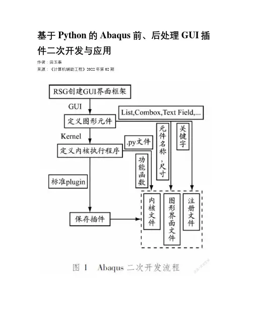
基于Python的Abaqus前、后处理GUI插件二次开发与应用作者：***来源：《计算机辅助工程》2022年第02期摘要：为提高Abaqus建模效率并进行可视化数据分析，利用Python语言对Abaqus前-后处理进行二次开发。

分析某柴油机机油-水冷却器模块组件，结果表明：前处理模块开发螺栓GUI插件，能够批量创建相同规格的螺栓载荷，提高前期建模效率，缩短分析周期;后处理模块开发Campbell制图插件，能根据工程实际需要将模态结果数据绘制成Campbell图，并将计算结果可视化输出。

关键词： Abaqus; Python; 二次开发; 前处理; 后处理; GUI界面中图分类号： TP391.99; TB115.1文献标志码： BGUI plugin redevelopment and application of Abaquspre-and post-processing based on PythonTIAN Yutai（Shanghai New Power Automotive Technology Co.， Ltd.， Shanghai 200438， China）Abstract： To improve the efficiency of Abaqus modeling and achieve visual data analysis，redevelopment of Abaqus pre-and post-processing is carried out with Python language. A diesel engine oil-water cooler module is analyzed. The results show that： a bolt GUI plug-in is developed for the pre-processing module， which can create bolt loads of the same specification in bulk，improving pre-modeling efficiency and shortening the analysis cycle; the Campbell mapping plug-in is investigated for the post-processing module， which can draw the modal result data into Campbell diagrams according to the actual needs of engineering and visualize the calculation results for output.Key words： Abaqus;Python; redevelopment; pre-processing;post-processing; GUI interface0引言作为国际通用计算分析软件，Abaqus具有丰富的单元类型与材料非线性模型，在各领域发挥至关重要的作用。

Abaqus二次开发——Abaqus/python入门体会入门实例#===========================================================自己的论文要用到有限元进行数值模拟分析，以前都用ansys计算，可ansys中岩土的本构模型只有D－P模型，无法准确的反映土的硬化/软化性质，模拟计算出的结果因此也和实际差别很大。

Abaqus有着丰富的材料模型，超强的非线性分析能力，岩土的模型也很多，因此才转学Abaqus。

Abaqus的cae建模功能还是很好的，但科研课题一般都要进行参数分析，采用cae的建模方法有些不切实际，学了没几天就放弃cae开始学习inp，也是学了一阵子才知道inp不能建立实体模型，只能直接建节点和单元。

复杂的模型inp也无法建立，但采用Python建模就可以解决这个问题。

由于Abaqus的学习资料不多，过了好些日子才知道Abaqus也可以采用Python语言进行建模计算，只是比Ansys的Apdl语言复杂得多，并且除了手册上的Script资料之外，没有较为系统的教程，刚一接触真是让人头痛。

通过查看Simwe论坛上关于Python的帖子，和论坛朋友的帮助，自己在慢慢积累，现在对Python有了一点点了解，算是入了个门。

接触Abaqus也没多久，对python更是一知半解，绝大多数地方根本都不清楚，抽空写一点认识体会主要是给像自己一样刚学习Abqus Python的朋友，能少走一些弯路，节约一些时间。

同时希望大家批评指正、共同讨论、补充。

#--------------------------------------------------------------------------------------------------学习Abaqus/Python基础：Abaqus的cae建模有比较全面的认识；了解一些Python语法知识（大家都不会有太多时间单独学习Python语言本身，只需要有概念了解即可，不懂的地方可以随时查询Python script手册）Abaqus/Python学会使用不太难，可要精通应用还是要付出一定的劳动。

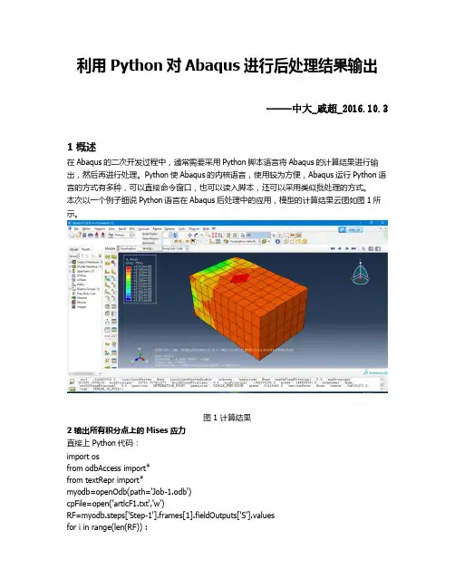
利用Python对Abaqus进行后处理结果输出-----中大_戚超_2016.10.31 概述在Abaqus的二次开发过程中，通常需要采用Python脚本语言将Abaqus的计算结果进行输出，然后再进行处理。

Python使Abaqus的内核语言，使用较为方便，Abaqus运行Python语言的方式有多种，可以直接命令窗口，也可以读入脚本，还可以采用类似批处理的方式。

本次以一个例子细说Python语言在Abaqus后处理中的应用，模型的计算结果云图如图1所示。

图1 计算结果2 输出所有积分点上的Mises应力直接上Python代码：import osfrom odbAccess import*from textRepr import*myodb=openOdb(path='Job-1.odb')cpFile=open('artlcF1.txt','w')RF=myodb.steps['Step-1'].frames[1].fieldOutputs['S'].valuesfor i in range(len(RF)) :cpFile.write('%.3F\n' %(RF[i].mises))else:cpFile.close()#引入模块，因为需要打开结果文件#打开结果文件，并复制给变量myodb#打开一个txt文件#将输出场赋值给RF#循环语句，向txt文件逐行写入mises应力Abaqus的结构层次分的很细，比如结果文件下分如下：使用过Abaqus的都知道step表示载荷步，frame表示载荷子步，因而在读取Mises应力时需要详细地指定输出哪一步的应力，而应力结果是输出场数据（fieldOutput）的中一种，需要指定是何种应力，程序才知道怎么读取并写入。

由于Abaqus里面涉及的变量特别多，通常很难记清楚那一项下面都有哪些量可以调用，此时比较好的方式是采用print 函数查看，例如查看myodb.steps['Step-1'].frames[1].fieldOutputs 下面有哪些变量可以调用，在窗口输入：print myodb.steps['Step-1'].frames[1].fieldOutputs显示：{'AC YIELD': 'FieldOutput object', 'CF': 'FieldOutput object', 'E': 'FieldOutput object', 'PE': 'Fiel dOutput object', 'PEEQ': 'FieldOutput object', 'PEMAG': 'FieldOutput object', 'RF': 'FieldOutput object', 'S': 'FieldOutput object', 'U': 'FieldOutput object'}各种不同的结果，包括位移、应力和支反力等等，因此可以知道通过如下的方式读取应力：myodb.steps['Step-1'].frames[1].fieldOutputs ['S']此时读取的信息特别多，我们想要的是其中的数值信息，因此可以：myodb.steps['Step-1'].frames[1].fieldOutputs ['S'].values通过此句能够读取所有节点的应力数据，输出其中一个：print myodb.steps['Step-1'].frames[1].fieldOutputs ['S'].values[0]显示：({'baseElementType': 'C3D8R', 'conjugateData': None, 'conjugateDataDouble': 'unknown', 'da ta': array([-855397.25, 58.817497253418, 358.723419189453, -139.652938842773, -456.986175537109, 4.29301929473877], 'f'), 'dataDouble': 'unknown', 'elementLabel': 1, 'fac e': None, 'instance': 'OdbInstance object', 'integrationPoint': 1, 'inv3': -855606.3125, 'localCoordSystem': None, 'localCoordSystemDouble': 'unknown', 'magnitude': None, 'maxInPlanePrincipal': 0.0, 'maxPrincipal': 359.0310********, 'midPrincipal': 58.7767 486572266, 'minInPlanePrincipal': 0.0, 'minPrincipal': -855397.5, 'mises': 855606.375, 'nodeLabel': None, 'outOfPlanePrincipal': 0.0, 'position': INTE GRATION_POINT, 'precision': SINGLE_PRECISION, 'press': 284993.25, 'sectionPoint': None, 'tr esca': 855756.5, 'type': TENSOR_3D_FULL})输出的信息特别多，但是可以看到有mises这一项。

abaqus-python二次开发方法（超实用）基于的二次开发对于很多新手来说都是一个神秘的，感觉是高难度的问题，致使很多新手对二次开发的研究都处于初级了解阶段，或完全不感冒阶段。

其实二次开发很简单，某种意义上讲，常用的ABAQUS二次开发方式有两种，（1）直接修改inp文件，这种方式需要对inp文件中大量的节点和单元进行操作，一般不建议采用inp文件进行二次开发（除非有特殊的关键字或标识符，其实关键字也可以用python语言来进行二次开发，笔者亲证）。

采用inp文件进行二次开发数据量大，行数多，一旦发生问题难以检测错误原因（2）采用abaqus语言，自编脚本，简单容易，非常适合初学者。

这里主要介绍python入门python语言的开发远没有想象中的难，其实基于abaqus语言的二次开发更像是word或excel里的VBA，我们只要通过录制一段宏文件，就可以简单迅速的完成一个模型的建立，当我们人为的对这段宏文件进行修改，就可以完成对该模型的修改，非常适合有大量相同或类似模型的建立，防止用户一遍又一遍繁琐的建模操作。

简单的步骤如下：1.在建模前先打开file--Macro Manager，然后新建一个宏文件（在Home或Work都行，只要你最终能找到这个文件），此时会弹出Record Macro对话框，托至不碍事的地方2.进行正常的cae建模就行，至到建模完成3.点击Record Macro对话框的Stop Mecording，此时命令栏会显示“Macro "Macroname" has been added to "E:\Temp\Macroname.py"”，前期任务搞定4.此时用文本编辑器打开此py文件，py文件中有些文字是没有用的，把“def Macro1 ...import connectorBehavior”都可以删掉，每行字前的空格都要去掉（文本编辑器里一般有列模式，用列模式可以对整个文本的进行操作）5.复制你新生成的python文件，并对该文件中的参数进行修改，在提交给abaqus--cae就可以完成重复建模了，如此可以无限重复，其实python语言都是大白话，你能看懂的需要指出的是：1.可以结合其它编程语言如VB、VC 配合修改参数并生成py文件，使用更为灵活2.生成py文件可以直接在cae中选择file-run script，选择你生成的python文件3.可以用python文件直接生成cae模型文件，可在py文件最后添加"mdb.saveAs(pathName='" *** "')"4.可以通过cmd命令直接将py文件提交个abaqus内核，让abaqus进行运算，cmd命令为“Shell"C:\Windows\SysWOW64\cmd.exe /k abaqus cae noGUI=" **** ".py ", vbHide等待abaqus运算的py语言"myJob.submit(consistencyChecking=OFF, datacheckJob=True)"。

Python语言在ABAQUS中的应用采用python脚本语言二次开发ABAQUS，通过开发python脚本程序处理ABAQUS重复工作，提高了工作效率。

标签Python；ABAQUS；交换输入；函数引言ABAQUS是大型通用的有限元分析软件，可以模拟绝大部分工程材料的线性和非线性行为，获得了广大用户的认可，在建筑结构分析领域应用广泛。

Python是一种面向对象的脚本语言，，该语言已经诞生20余年，它的简洁性和易用性使程序的开发过程变得简单，特别适用于快速应用开发。

在此介绍一下编写脚本快速建模。

编写Python脚本快速建立模型是ABAQUS高级用户经常使用的功能之一。

例如，在Abaqus/CAE中建模时需要反复输入各种参数和设置多个对话框，编写脚本只需要几条语句就可以实现。

如果经常建立相同或类似模型，还可以编写独立的模块，还可以编写脚本创建材料库，运行Python脚本后Material Manager 将自动出现定义的材料。

在此介绍3种最常用的快速建立模型的方法，包括交互式输入、创建材料库。

1.交互式输入交互式输入直接指定模型参数，而无需在Abaqus/CAE下选择多个菜单、多个按钮，可以节省许多建模时间。

Abaqus脚本接口提供3种交互式输入函数，分别是：getInput（）函数、getInputs（）函数和getWarningReply （）函数，详细介绍参见Abaqus 6.10帮助手册《Abaqus Scripting User’s Manual》第6.7节“Prompting the user for input”和<《Abaqus Scripting Reference Manual》第49.5节“User input commands”。

GetInput（）函数脚本getInput.py将调用getInput（）函数自定义输入参数，开平方根运算后输出计算结果。

程序测试代码如下：from abaqus import *from math import sqrtinput=getInput（’please enter a number ‘，’9’）number=float（input）print sqrt（number）GetInputs（）函数脚本getInputs.py将调用getInputs（）函数自定义输入并输出数据信息，代码如下：from abaqus import *x=getInputs（（（’please enter the first number ‘，’2’），（’please enter the second number’，’5’），（’please enter the third number’，’8’）））print xGetWarningReply （）函数脚本getWarningReply.py将调用get Warning Reply （）函数来创建警告对话框。

Python语言和ABAQUS后处理二次开发1易桂莲杜家政隋允康2（北京工业大学机械工程与应用电子技术学院，100124北京）摘要：采用Python脚本语言二次开发ABAQUS的后处理模块，讨论了ABAQUS的脚本接口和对象模型在二次开发中的作用和调用流程。

通过开发Python脚本程序提取ABAQUS进行数值模拟后的计算结果，有效地解决了提取大量结果进行重复操作的问题，提高了后处理的效率。

关键词：ABAQUS后处理二次开发；Python；动力响应分析；振动特性0 引言ABAQUS是国际上最先进的大型通用有限元计算分析软件之一,可以模拟绝大部分工程材料的线性和非线性行为。

ABAQUS自带的CAE是进行有限元分析的前后处理模块,也是建模、分析和后处理的人机交互平台,它具有良好的人机对话界面,因此ABAQUS软件在工程中得到了广泛的应用。

Python是一种面向对象的脚本语言,它功能强大,既可以独立运行,也可以用作脚本语言。

特别适用于快速的应用程序开发[1]。

通过开发Python脚本程序提取ABAQUS进行数值模拟后的计算结果，有效地解决了提取大量结果进行重复操作的问题1 二次开发接口介绍ABAQUS 脚本接口是一个基于对象的程序库,脚本接口中的每个对象都拥有相应的数据成员和函数。

对象的函数专门用于处理对象中的数据成员，被称为相应对象的方法，用于生成对象的方法被称为构造函数。

在对象创建后，可以使用该对象提供的方法来处理对象中的数据成员[2]。

ABAQUS提供了一套应用程序编程接口(API，Application Program Interface)来操作ABAQUS/CAE实现建模/后处理等功能。

接口编程采用Python的语法编写脚本，但扩展了Python脚本语言，额外提供了大约500个对象模型。

对象模型之间关系复杂，图1展示了这些对象模型之间的层次结构和相互关系。

其中，Container表示容器，里面包含有其他的对象；Singular object表示单个对象。

基于Python的Abaqus二次开发实例讲解（asian58 2013.6.26）基于Python的Abaqus的二次开发便捷之处在于：1、所有的代码均可以先在Abaqus\CAE中操作一遍后再通过rp文件读取，然后再在此基础上进行相应的修改；2、Python是一种解释性语言，读起来非常清晰，因此在修改程序的过程中，不存在程序难以理解的问题；3、Python是一种通用性的、功能非常强大的面向对象编程语言，有许多成熟的类似于Matlab函数的程序在网络上流传，为后期进一步的数据处理提供了方便。

为了更加方便地完成Abaqus的二次开发，需进行一些相关约定：1、所有参数化直接通过点的坐标值进行，直接对几何尺寸的参数化反而更加繁琐；2、程序参数化已不允许在模型中添加太多的Tie，因此不同零部件的绑定直接通过共节点来进行，这就要求建模方法与常规的建模方法有所区别。

思路如下：将一个整机拆成几个大的Part来建立，一个Part中包含许多零件，这样在划分网格式时就可以自动实现共节点的绑定。

不同的零件可通过建立不同的Set来进行区分，不同Part 的绑定可以通过Tie来实现。

将一个复杂的结构拆成几个恰当的Part来建立，一方面可以将复杂的模型简单化，使建立复杂模型成为可能；另一方面，不同的Part可单独调用，从而又可实现程序的模块化，增加程序的适应范围，延长程序的使用寿命，也方便后期程序的维护和修改。

3、通过py文件建立起的模型要进行参数优化，已不适合采用Isight中Abaqus模块，需要用到Isight的Simcode模块。

下面详细解释一个臂架的py文件。

#此程序用来绘制臂架前段#导入相关模块# -*- coding: mbcs -*-from abaqus import *from abaqusConstants import *#定义整个臂架的长、宽、高L0=14300W0=1650H0=800#创建零件P01_12 L1=H0+200 W1=200 T1=12s = mdb.models['Model-1'].ConstrainedSketch(name='__profile__', sheetSize=2000.0)g, v, d, c = s.geometry, s.vertices, s.dimensions, s.constraints s.setPrimaryObject(option=STANDALONE)s.rectangle(point1=(W0/2, L1/2), point2=(W0/2+W1, -L1/2))s.rectangle(point1=(-W0/2, L1/2), point2=(-W0/2-W1, -L1/2))p = mdb.models['Model-1'].Part(name='Part-1', dimensionality=THREE_D, type=DEFORMABLE_BODY)p = mdb.models['Model-1'].parts['Part-1'] p.BaseShell(sketch=s)session.viewports['Viewport: 1'].setValues(displayedObject=p) del mdb.models['Model-1'].sketches['__profile__']#定义零件的厚度p = mdb.models['Model-1'].parts['Part-1'] f = p.faces pickedFaces01 = f.findAt (((W0/2, L1/2, 0),),((-W0/2, L1/2, 0),), ) p.assignThickness(faces=pickedFaces01, thickness=T1) p.Set(faces=pickedFaces01, name='P01_12')#创建辅助平面和辅助坐标系p = mdb.models['Model-1'].parts['Part-1']p.DatumCsysByThreePoints(name='Datum csys-1', coordSysType=CARTESIAN, origin=( 0.0, 0.0, 0.0), line1=(1.0, 0.0, 0.0), line2=(0.0, 1.0, 0.0))p = mdb.models['Model-1'].parts['Part-1']p.DatumPlaneByPrincipalPlane(principalPlane=XYPLANE, offset=L0)#创建零件P02_12 L2=L1 W2=W1 T2=12p = mdb.models['Model-1'].parts['Part-1'] d = p.datums#将草图原点参数化t = p.MakeSketchTransform(sketchPlane=d[5], sketchUpEdge=d[4].axis2, sketchPlaneSide=SIDE1, sketchOrientation=RIGHT, origin=(0.0, 0.0, L0)) s = mdb.models['Model-1'].ConstrainedSketch(name='__profile__', sheetSize=29006.85, gridSpacing=725.17, transform=t) g, v, d1, c = s.geometry, s.vertices, s.dimensions, s.constraints s.setPrimaryObject(option=SUPERIMPOSE)p = mdb.models['Model-1'].parts['Part-1']s.rectangle(point1=(W0/2, L2/2), point2=(W0/2+W2, -L2/2))s.rectangle(point1=(-W0/2, L2/2), point2=(-W0/2-W2, -L2/2))p = mdb.models['Model-1'].parts['Part-1']d2 = p.datumsp.Shell(sketchPlane=d2[5], sketchUpEdge=d2[4].axis2, sketchPlaneSide=SIDE1, sketchOrientation=RIGHT, sketch=s)s.unsetPrimaryObject()del mdb.models['Model-1'].sketches['__profile__']#定义零件的厚度p = mdb.models['Model-1'].parts['Part-1'] Array f = p.facespickedFaces02 = f.findAt(((W0/2, L1/2, L0),),((-W0/2, L1/2, L0),), )p.assignThickness(faces=pickedFaces02, thickness=T2)p.Set(faces=pickedFaces02, name='P02_12')#创建零件P03_12和零件P04_08T3=12T4=8p = mdb.models['Model-1'].parts['Part-1']d = p.datumst = p.MakeSketchTransform(sketchPlane=d[5], sketchUpEdge=d[4].axis2, sketchPlaneSide=SIDE1, sketchOrientation=RIGHT, origin=(0.0, 0.0, L0)) s = mdb.models['Model-1'].ConstrainedSketch(name='__profile__', sheetSize=29006.85, gridSpacing=725.17, transform=t)g, v, d1, c = s.geometry, s.vertices, s.dimensions, s.constraintss.setPrimaryObject(option=SUPERIMPOSE)#创建草图p = mdb.models['Model-1'].parts['Part-1']s.Line(point1=(-W0/2-W1, H0/2), point2=(-W0/2, H0/2))s.Line(point1=(W0/2, H0/2), point2=(W0/2+W1, H0/2))s.Line(point1=(-W0/2-W1, -H0/2), point2=(-W0/2, -H0/2))s.Line(point1=(W0/2, -H0/2), point2=(W0/2+W1, -H0/2))p = mdb.models['Model-1'].parts['Part-1']d2 = p.datumsp.ShellExtrude(sketchPlane=d2[5], sketchUpEdge=d2[4].axis2,sketchPlaneSide=SIDE1, sketchOrientation=RIGHT, sketch=s, depth=L0, flipExtrudeDirection=ON)s.unsetPrimaryObject()del mdb.models['Model-1'].sketches['__profile__']#定义零件P03_12的厚度p = mdb.models['Model-1'].parts['Part-1']f = p.facespickedFaces03 = f.findAt(((-W0/2, H0/2, L0/2),),((W0/2, H0/2, L0/2),),)p.assignThickness(faces=pickedFaces03, thickness=T3)p.Set(faces=pickedFaces03, name='P03_12')#定义零件P04_12的厚度p = mdb.models['Model-1'].parts['Part-1']f = p.facespickedFaces04 = f.findAt(((-W0/2, -H0/2, L0/2),),((W0/2, -H0/2, L0/2),),)p.assignThickness(faces=pickedFaces04, thickness=T4)p.Set(faces=pickedFaces04, name='P04_12')#创建零件P05_08T5=8p = mdb.models['Model-1'].parts['Part-1']d = p.datumst = p.MakeSketchTransform(sketchPlane=d[5], sketchUpEdge=d[4].axis2, sketchPlaneSide=SIDE1, sketchOrientation=RIGHT, origin=(0.0, 0.0, L0))s = mdb.models['Model-1'].ConstrainedSketch(name='__profile__',sheetSize=29006.85, gridSpacing=725.17, transform=t)g, v, d1, c = s.geometry, s.vertices, s.dimensions, s.constraintss.setPrimaryObject(option=SUPERIMPOSE)p = mdb.models['Model-1'].parts['Part-1']s.Line(point1=(-W0/2-W1/2, H0/2), point2=(-W0/2-W1/2, -H0/2))s.Line(point1=(W0/2+W1/2, H0/2), point2=(W0/2+W1/2, -H0/2))p = mdb.models['Model-1'].parts['Part-1']d2 = p.datumsp.ShellExtrude(sketchPlane=d2[5], sketchUpEdge=d2[4].axis2,sketchPlaneSide=SIDE1, sketchOrientation=RIGHT, sketch=s, depth=L0,flipExtrudeDirection=ON)s.unsetPrimaryObject()del mdb.models['Model-1'].sketches['__profile__']#定义零件P05_8的厚度p = mdb.models['Model-1'].parts['Part-1']f = p.facespickedFaces05 = f.findAt(((-W0/2-W1/2, 0, L0/2),),((W0/2+W1/2, 0, L0/2),),)p.assignThickness(faces=pickedFaces05, thickness=T5)p.Set(faces=pickedFaces05, name='P05_08')#创建零件P06_08L6=W0+W1n=L0//2520+1T6=8p = mdb.models['Model-1'].parts['Part-1']f, d = p.faces, p.datumst = p.MakeSketchTransform(sketchPlane=f[0], sketchUpEdge=d[4].axis2, sketchPlaneSide=SIDE1, sketchOrientation=RIGHT, origin=(W0/2+W1/2, -H0/2,0))s = mdb.models['Model-1'].ConstrainedSketch(name='__profile__',sheetSize=28684, gridSpacing=717, transform=t)g, v, d1, c = s.geometry, s.vertices, s.dimensions, s.constraintss.setPrimaryObject(option=SUPERIMPOSE)p = mdb.models['Model-1'].parts['Part-1']#循环命令绘制平行隔板for i in range(0,n): Array s.Line(point1=(-500-(i*2520), H0), point2=(-500-(i*2520), 0.0))p = mdb.models['Model-1'].parts['Part-1']f1, d2 = p.faces, p.datumsp.ShellExtrude(sketchPlane=f1[0], sketchUpEdge=d2[4].axis2,sketchPlaneSide=SIDE1, sketchOrientation=RIGHT, sketch=s, depth=L6,flipExtrudeDirection=ON)s.unsetPrimaryObject()del mdb.models['Model-1'].sketches['__profile__']#定义零件P06_08的厚度p = mdb.models['Model-1'].parts['Part-1']f = p.facesfor i in range(0,n): Array pickedFaces = f.findAt(((0, H0/4, 500+i*2520),))p.assignThickness(faces=pickedFaces, thickness=T6)p.Set(faces=pickedFaces, name='P06_08_'+str(1+i))#创建零件P07_12,P08_12W7=200L7=W0+W1T7=12T8=12p = mdb.models['Model-1'].parts['Part-1']f, e = p.faces, p.edgest = p.MakeSketchTransform(sketchPlane=f.findAt(coordinates=(W0/2+W1/2, 0.0, 100.0)),sketchUpEdge=e.findAt(coordinates=(W0/2+W1/2, 0.0, 0.0)),sketchOrientation=RIGHT,sketchPlaneSide=SIDE1,origin=(W0/2+W1/2, -H0/2, 0.0))s = mdb.models['Model-1'].ConstrainedSketch(name='__profile__',sheetSize=53678, gridSpacing=1341, transform=t)g, v, d, c = s.geometry, s.vertices, s.dimensions, s.constraintss.setPrimaryObject(option=SUPERIMPOSE)p = mdb.models['Model-1'].parts['Part-1']#循环命令绘制平行隔板for i in range(0,n):s.Line(point1=(400+i*2520, -H0), point2=(600+i*2520, -H0))s.Line(point1=(400+i*2520, 0), point2=(600+i*2520, 0))p = mdb.models['Model-1'].parts['Part-1']f1, e1 = p.faces, p.edgesp.ShellExtrude(sketchPlane=f.findAt(coordinates=(W0/2+W1/2, 0.0, 100.0)),sketchUpEdge=e.findAt(coordinates=(W0/2+W1/2, 0.0, 0.0)),sketchPlaneSide=SIDE1,sketchOrientation=RIGHT, sketch=s, depth=W0+W1, flipExtrudeDirection=ON, keepInternalBoundaries=ON)s.unsetPrimaryObject()del mdb.models['Model-1'].sketches['__profile__']#定义零件P07_12的厚度p = mdb.models['Model-1'].parts['Part-1']f = p.facesfor i in range(0,n):pickedFaces07 = f.findAt(((0, H0/2, 400+i*2520),),((0, H0/2, 600+i*2520),),) p.assignThickness(faces=pickedFaces07, thickness=T7)p.Set(faces=pickedFaces07, name='P07_12_'+str(1+i))fp=[]for i in range(0,2):fp.append(f.findAt(((0, H0/2, 400+i*2520),),((0, H0/2, 600+i*2520),),))p.Set(faces=fp, name='P07_fp')#定义零件P08_12的厚度p = mdb.models['Model-1'].parts['Part-1']f = p.facesfor i in range(0,n):pickedFaces08 = f.findAt(((0, -H0/2, 400+i*2520),),((0, -H0/2, 600+i*2520),),) p.assignThickness(faces=pickedFaces08, thickness=T7)p.Set(faces=pickedFaces08, name='P08_12_'+str(1+i))#为中间隔板创建空腔#定义相关参数边界距离、圆角d0=100r0=100p = mdb.models['Model-1'].parts['Part-1']f1, e1 = p.faces, p.edgest = p.MakeSketchTransform(f.findAt(coordinates=(0, 0.0, 500.0)),sketchUpEdge=e.findAt(coordinates=(W0/2+W1/2, 0.0, 500.0)),sketchPlaneSide=SIDE1, sketchOrientation=RIGHT,origin=(0.0, 0.0, 500.0))s = mdb.models['Model-1'].ConstrainedSketch(name='__profile__',sheetSize=5910.0, gridSpacing=147.0, transform=t)g, v, d1, c = s.geometry, s.vertices, s.dimensions, s.constraintss.setPrimaryObject(option=SUPERIMPOSE)p = mdb.models['Model-1'].parts['Part-1']p.projectReferencesOntoSketch(sketch=s, filter=COPLANAR_EDGES)#创建矩形s.rectangle(point1=(-W0/2-W1/2+d0, H0/2-d0), point2=(W0/2+W1/2-d0, -H0/2+d0)) #创建圆角s.FilletByRadius(radius=r0,curve1=g[29], nearPoint1=(-W0/2-W1/2+d0, H0/2-d0), curve2=g[26], nearPoint2=(-W0/2-W1/2+d0, H0/2-d0))s.FilletByRadius(radius=r0, curve1=g[26], nearPoint1=(-W0/2-W1/2+d0, -H0/2+d0), curve2=g[27], nearPoint2=(-W0/2-W1/2+d0, -H0/2+d0)) s.FilletByRadius(radius=r0, curve1=g[27], nearPoint1=(W0/2+W1/2-d0, -H0/2+d0), curve2=g[28], nearPoint2=(W0/2+W1/2-d0, -H0/2+d0)) s.FilletByRadius(radius=r0, curve1=g[28], nearPoint1=(W0/2+W1/2-d0, H0/2-d0), curve2=g[29], nearPoint2=(W0/2+W1/2-d0, H0/2-d0))p = mdb.models['Model-1'].parts['Part-1']f1, d2 = p.faces, p.datumsp.CutExtrude(f.findAt(coordinates=(0, 0.0, 500.0)),sketchUpEdge=e.findAt(coordinates=(W0/2+W1/2, 0.0, 500.0)),sketchPlaneSide=SIDE1, sketchOrientation=RIGHT, sketch=s, depth=L0, flipExtrudeDirection=OFF)s.unsetPrimaryObject()del mdb.models['Model-1'].sketches['__profile__']#开始建立梁Beam_1p = mdb.models['Model-1'].parts['Part-1']f, d = p.faces, p.datums#绘制参考面p.DatumPlaneByOffset(plane=f.findAt(coordinates=(W0/2, -H0/2, 100.0)),flip=SIDE2, offset=8.0)dp1 = d.keys()[-1]p = mdb.models['Model-1'].parts['Part-1']d = p.datumst = p.MakeSketchTransform(sketchPlane=d[dp1], sketchUpEdge=d[4].axis1,sketchPlaneSide=SIDE1, sketchOrientation=RIGHT, origin=(0.0, 0.0,0.0))s = mdb.models['Model-1'].ConstrainedSketch(name='__profile__', sheetSize=31857.0, gridSpacing=796.0, transform=t)g, v, d1, c = s.geometry, s.vertices, s.dimensions, s.constraintss.setPrimaryObject(option=SUPERIMPOSE)p = mdb.models['Model-1'].parts['Part-1']#计算中间加强梁的数量if n%2==1:n1=n//2 n2=n//2 else:n1=n//2 n2=n//2-1 for i in range(0,n1):s.Line(point1=(-500-i*2520*2, W0/2+W1/2), point2=(-500-2520-i*2520*2,-W0/2-W1/2 )) for i in range(0,n2):s.Line(point1=(-500-2520-i*2520*2,-W0/2-W1/2), point2=(-500-2*2520-i*2520*2,W0/2+W1/2 ))#在基准平面dp1上面绘制梁p = mdb.models['Model-1'].parts['Part-1'] d2 = p.datums e = p.edgesp.Wire(sketchPlane=d2[dp1], sketchUpEdge=d2[4].axis1, sketchPlaneSide=SIDE1, sketchOrientation=RIGHT, sketch=s) s.unsetPrimaryObject()del mdb.models['Model-1'].sketches['__profile__'] edges1=[] for i in range(0,n-1): edges1.append (e.findAt(((0, -H0/2-8, 500+2520/2+i*2520),),)) p.Set(edges=edges1, name='Beam_1') ############################开始定义有限元分析的相关参数 #定义材料mdb.models['Model-1'].Material(name='steel')mdb.models['Model-1'].materials['steel'].Elastic(table=((210000.0, 0.3), )) mdb.models['Model-1'].materials['steel'].Density(table=((7.8e-06, ), ))#定义壳单元属性mdb.models['Model-1'].HomogeneousShellSection(name='shell', preIntegrate=OFF, material='steel', thicknessType=UNIFORM, thickness=10.0, thicknessField='', idealization=NO_IDEALIZATION, poissonDefinition=DEFAULT,thicknessModulus=None, temperature=GRADIENT, useDensity=OFF, integrationRule=SIMPSON, numIntPts=5) #赋所有壳单元属性p = mdb.models['Model-1'].parts['Part-1']for i in range(1,5):region1 = p.sets['P0'+str(i)+'_12']p.SectionAssignment(region=region1, sectionName='shell', offset=0.0,offsetType=FROM_GEOMETRY , offsetField='',thicknessAssignment=FROM_GEOMETRY )region2 = p.sets['P05_08']p.SectionAssignment(region=region2, sectionName='shell', offset=0.0, offsetType=FROM_GEOMETRY, offsetField='',thicknessAssignment=FROM_GEOMETRY)for i in range(1,n+1): Array region3 = p.sets['P06_08_'+str(i)]p.SectionAssignment(region=region3, sectionName='shell', offset=0.0,offsetType=FROM_GEOMETRY, offsetField='',thicknessAssignment=FROM_GEOMETRY)for i in range(1,n+1):region4 = p.sets['P07_12_'+str(i)]p.SectionAssignment(region=region4, sectionName='shell', offset=0.0,offsetType=FROM_GEOMETRY, offsetField='',thicknessAssignment=FROM_GEOMETRY)for i in range(1,n+1):region5 = p.sets['P08_12_'+str(i)]p.SectionAssignment(region=region5, sectionName='shell', offset=0.0,offsetType=FROM_GEOMETRY, offsetField='',thicknessAssignment=FROM_GEOMETRY)#定义梁单元属性mdb.models['Model-1'].LProfile(name='L_65', a=65.0, b=65.0, t1=7.0, t2=7.0)mdb.models['Model-1'].BeamSection(name='B_65', integration=DURING_ANALYSIS,poissonRatio=0.0, profile='L_65', material='steel', temperatureVar=LINEAR,consistentMassMatrix=False)#赋所有梁单元属性p = mdb.models['Model-1'].parts['Part-1']region = p.sets['Beam_1']p.SectionAssignment(region=region, sectionName='B_65', offset=0.0,offsetType=MIDDLE_SURFACE, offsetField='',thicknessAssignment=FROM_SECTION)p.assignBeamSectionOrientation(region=region, method=N1_COSINES, n1=(0.0, 0.0,-1.0))#定义装配体import assemblya = mdb.models['Model-1'].rootAssemblya.DatumCsysByDefault(CARTESIAN)p = mdb.models['Model-1'].parts['Part-1']a.Instance(name='Part-1-1', part=p, dependent=ON)#定义分析步import stepmdb.models['Model-1'].StaticStep(name='Step-1', previous='Initial')#定义底面与梁的tiedimport interactiona = mdb.models['Model-1'].rootAssemblyregion1=a.instances['Part-1-1'].sets['P04_12']region2=a.instances['Part-1-1'].sets['Beam_1']mdb.models['Model-1'].Tie(name='Constraint-1', master=region1, slave=region2, positionToleranceMethod=COMPUTED, adjust=OFF, tieRotations=ON, thickness=ON)#开始定义耦合#导入相关模块import regionToolseta = mdb.models['Model-1'].rootAssemblyd, r = a.datums, a.referencePoints#定义参考点a.ReferencePoint(point=(0.0, H0/2, 500+2520/2))rp1 = r.keys()[-1]refPoints1=(r1[rp1], )region1=regionToolset.Region(referencePoints=refPoints1)s1 = a.instances['Part-1-1'].facesregion2 = a.instances['Part-1-1'].sets['P07_fp']mdb.models['Model-1'].Coupling(name='Constraint-2', controlPoint=region1, surface=region2, influenceRadius=WHOLE_SURFACE, couplingType=DISTRIBUTING, localCsys=None, u1=ON, u2=ON, u3=ON, ur1=ON, ur2=ON, ur3=ON)#########################定义边界条件import loada = mdb.models['Model-1'].rootAssemblyd, r = a.datums, a.referencePointsregion = a.instances['Part-1-1'].sets['P02_12']mdb.models['Model-1'].DisplacementBC(name='SPC', createStepName='Initial', region=region, u1=SET, u2=SET, u3=SET, ur1=SET, ur2=SET, ur3=SET,amplitude=UNSET, distributionType=UNIFORM, fieldName='', localCsys=None)a = mdb.models['Model-1'].rootAssemblyregion = a.instances['Part-1-1'].sets['P08_12_'+str(n-1)]mdb.models['Model-1'].DisplacementBC(name='SPC2', createStepName='Initial', region=region, u1=SET, u2=SET, u3=SET, ur1=SET, ur2=SET, ur3=SET,amplitude=UNSET, distributionType=UNIFORM, fieldName='', localCsys=None)r1 = a.referencePointsrefPoints1=(r1[rp1], )region = regionToolset.Region(referencePoints=refPoints1)mdb.models['Model-1'].ConcentratedForce(name='force', createStepName='Step-1',region=region, cf2=-10000.0, distributionType=UNIFORM, field='',localCsys=None)mdb.models['Model-1'].Gravity(name='G', createStepName='Step-1', comp2=-9.8, distributionType=UNIFORM, field='')#################划分网格import meshp = mdb.models['Model-1'].parts['Part-1']p.seedPart(size=20.0, deviationFactor=0.1, minSizeFactor=0.1)p.generateMesh()a = mdb.models['Model-1'].rootAssembly###############创建作业并提交分析import jobmdb.Job(name='006', model='Model-1', description='', type=ANALYSIS, atTime=None, waitMinutes=0, waitHours=0, queue=None, memory=90,memoryUnits=PERCENTAGE, getMemoryFromAnalysis=True,explicitPrecision=SINGLE, nodalOutputPrecision=SINGLE, echoPrint=OFF,modelPrint=OFF, contactPrint=OFF, historyPrint=OFF, userSubroutine='',scratch='', multiprocessingMode=DEFAULT, numCpus=4, numDomains=4) mdb.jobs['006'].submit(consistencyChecking=ON)mdb.jobs['006'].waitForCompletion()###############进入后处理模块import visualizationo3 = session.openOdb(name='F:/ABAQUS/006.odb')session.viewports['Viewport: 1'].setValues(displayedObject=o3)session.viewports['Viewport: 1'].odbDisplay.display.setValues(plotState=( CONTOURS_ON_DEF, ))session.viewports['Viewport: 1'].view.setValues(session.views['Iso'])mdb.saveAs(pathName='F:/ABAQUS/006.cae')第11 页共11 页。

ABAQUS二次开发教程ABAQUS（Python语言）二次开发人生苦短，我用Python作者：Fan Shengbao2017年12月目录Python程序基本语法1.1Python语法结构Python语言以缩进来约束每个程序块，编写程序时要特别注意每一行的缩进量，同一层次的语句应具有相同的缩进量。

下面是一段Python程序示例：#-*- coding:utf-8 -*-for i in range(1,10):for j in range(1,i+1):print str(j)+'x'+str(i)+' = '+str(i*j),print该段程序主要功能是实现乘法口诀表输出打印，其中“#-*- coding:utf-8 -*-”是约定文档的编码方式。

程序主体部分由两个嵌套的for循环语句组成，可以看到每一个for循环块的内部都具有相同的缩进量。

程序输出结果如下：1x1=11x2=2 2x2=41x3=3 2x3=6 3x3=91x4=4 2x4=8 3x4=12 4x4=161x5=5 2x5=10 3x5=15 4x5=20 5x5=251x6=6 2x6=12 3x6=18 4x6=24 5x6=30 6x6=361x7=7 2x7=14 3x7=21 4x7=28 5x7=35 6x7=42 7x7=491x8=8 2x8=16 3x8=24 4x8=32 5x8=40 6x8=48 7x8=56 8x8=641x9=9 2x9=18 3x9=27 4x9=36 5x9=45 6x9=54 7x9=638x9=72 9x9=81Python程序中一行中“#”号后面的内容为注释，“#”号只支持单行注释，多行注释可使用“’’’ …‘’’”注释符。

'''Python'''1.2P ython元组Python中的元组（tuple）相当于C语言中的数组简化版，其内容和长度均不可变，只能对其内容进行访问。

使用python进行ABAQUS的二次开发的简要说明（byYoung2017.06.27）（所有用词以英文为准，翻译仅供参考）一、abaqus二次开发总述：首先最重要的知识点需要明确，abaqus在求解核心（Solver/ Kernel）和图形用户界面（GUI）之间使用的交互语言天然就是python，因此使用python进行abaqus二次开发是十分自然的选择（当然你也可以用C++，但是鉴于python所拥有的各类开源库函数的优势，python应当是二次开发的首选）。

abaqus已经使用python 写好了很多用于计算、建模、GUI等操作的模块，因此二次开发的重点在于灵活调用这些模块，完成自己的设计计算需求。

所以原则上，所有能通过abaqus/CAE交互完成的操作，使用脚本都可以实现。

并且由于Python提供的丰富的函数资源库，会使得很多复杂的建模的过程更加参数化，更加可控，有时候甚至更加简单。

其次二次开发的学习要点在于勤查手册，其中Abaqus Scripting User's Manual和Abaqus Scripting User's Reference Manual是查阅的重点，其中后者是abaqus中各个object内置方法，路径，输入参数等的详细说明。

最后关于调用脚本的几种用法说明：(1)直接在命令行调用调用脚本并打开cae界面： abaqus cae script=myscript.py调用用于可视化操作脚本，打开显示界面（注意：此时只有visualization模块被激活）： abaqus cae viewer=myscript.py 调用脚本在命令行执行，同时不打开GUI界面，但会进入python 交互界面：abaqus cae noGUI=myscript.py(2)在abaqus的GUI界面调用按照Main Menu: File->Run Script，选择需要调用的脚本文件，abaqus会进行执行(3)在abaqus的命令行交互界面调用（command line interface，在abaqus的GUI界面打开之后，窗口的最下方会有命令输入的位置，在这里也可以调用python脚本，执行方法是键入命令：execfile('myscript.py')abaqus的python脚本其实和其他应用场景下的python脚本没有太多区别，只不过有很多abaqus已经开发好的对象库可供使用，其学习过程和学习任何其他python库都是一致的。

3.1 Creating a partThe first example shows how you can use an Abaqus/CAE script to replicate the functionality of Abaqus/CAE. The script does the following:∙Creates a new model in the model database.∙Creates a two-dimensional sketch.∙Creates a three-dimensional, deformable part.∙Extrudes the two-dimensional sketch to create the first geometric feature of the part.∙Creates a new viewport.∙Displays a shaded image of the new part in the new viewport. The new viewport and the shaded part are shown in Figure 3–1. Figure 3–1 The example creates a new viewport and a part.The example scripts from this manual can be copied to the user's working directory by using the Abaqus fetch utility:abaqus fetch job=scriptNamewhere scriptName.py is the name of the script (see “Execution procedure for fetching sample input files,” Section 3.2.12 of the Abaqus Analysis User's Manual). Use the following command to retrieve the script for this example:abaqus fetch job=modelAExampleNote: Abaqus does not install the sample scripts by default during the installation procedure. As a result, if the Abaqus fetch utility fails to find the sample script, the script may be missing from your Abaqus installation. You must rerun the installation procedure and request Abaqus sample problems from the list of items to install.To run the program, do the following:1.Start Abaqus/CAE by typing abaqus cae.2.From the startup screen, select Run Script.3.From the Run Script dialog box that appears, selectmodelAExample.py.4.Click OK to run the script.Note: If Abaqus/CAE is already running, you can run the script by selecting File Run Script from the main menu bar.3.1.1 The example script"""modelAExample.pyA simple example: Creating a part."""from abaqus import *import testUtilstestUtils.setBackwardCompatibility()from abaqusConstants import *import sketchimport partmyModel = mdb.Model(name='Model A')mySketch = myModel.ConstrainedSketch(name='Sketch A', sheetSize=200.0)xyCoordsInner = ((-5 , 20), (5, 20), (15, 0),(-15, 0), (-5, 20))xyCoordsOuter = ((-10, 30), (10, 30), (40, -30),(30, -30), (20, -10), (-20, -10),(-30, -30), (-40, -30), (-10, 30))for i in range(len(xyCoordsInner)-1):mySketch.Line(point1=xyCoordsInner[i],point2=xyCoordsInner[i+1])for i in range(len(xyCoordsOuter)-1):mySketch.Line(point1=xyCoordsOuter[i],point2=xyCoordsOuter[i+1])myPart = myModel.Part(name='Part A', dimensionality=THREE_D,type=DEFORMABLE_BODY)myPart.BaseSolidExtrude(sketch=mySketch, depth=20.0)myViewport = session.Viewport(name='Viewport for Model A',origin=(10, 10), width=150, height=100)myViewport.setValues(displayedObject=myPart)myViewport.partDisplay.setValues(renderStyle=SHADED)3.1.2 How does the script work?This section explains each portion of the example script.from abaqus import *This statement makes the basic Abaqus objects accessible to the script. It also provides access to a default model database using the variable named mdb. The statement, from abaqusConstants import *, makes the Symbolic Constants defined by the Abaqus Scripting Interface available to the script.import sketchimport partThese statements provide access to the objects related to sketches and parts. sketch and part are called Python modules.The next statement in the script is shown in Figure 3–2. You can read this statement from right to left as follows:1.Create a new model named Model A.2.Store the new model in the model database mdb.3.Assign the new model to a variable called myModel.Figure 3–2 Creating a new model.mySketch = myModel.ConstrainedSketch(name='Sketch A', sheetSize=200.0) This statement creates a new sketch object named Sketch A in myModel. The variable mySketch is assigned to the new sketch. The sketch will be placed on a sheet 200 units square. Note the following:∙ A command that creates something (an “object” in object-oriented programming terms) is called a constructor and starts with anuppercase character. You have seen the Model and Sketch commands that create Model objects and Sketch objects, respectively.∙The command uses the variable myModel that we created in the previous statement. Using variables with meaningful names in ascript makes the script easier to read and understand.xyCoordsInner = ((-5 , 20), (5, 20), (15, 0),(-15, 0), (-5, 20))xyCoordsOuter = ((-10, 30), (10, 30), (40, -30),(30, -30), (20, -10), (-20, -10),(-30, -30), (-40, -30), (-10, 30))These two statements define the X- and Y-coordinates of the vertices that form the inner and outer profile of the letter “A.” The variable xyCoordsInner refers to the vertices of the inner profile, and the variable xyCoordsOuter refers to the vertices of the outer profile. for i in range(len(xyCoordsInner)-1):mySketch.Line(point1=xyCoordsInner[i],point2=xyCoordsInner[i+1])This loop creates the inner profile of the letter “A” in mySketch. Four lines are created using the X- and Y-coordinates of the vertices in xyCoordsInner to define the beginning point and the end point of each line. Note the following:∙Python uses only indentation to signify the start and the end ofa loop. Python does not use the brackets {} of C and C++.∙The len() function returns the number of coordinate pairs in xyCoordsInner—five in our example.∙The range() function returns a sequence of integers. In Python, as in C and C++, the index of an array starts at zero. In our example range(4) returns 0,1,2,3. For each iteration of the loop in theexample the variable i is assigned to the next value in the sequence of integers.Similarly, a second loop creates the outer profile of the “A” character. myPart = myModel.Part(name='Part A',dimensionality=THREE_D, type=DEFORMABLE_BODY)This statement creates a three-dimensional, deformable part named Part A in myModel. The new part is assigned to the variable myPart. myPart.BaseSolidExtrude(sketch=mySketch, depth=20.0)This statement creates a base solid extrude feature in myPart by extruding mySketch through a depth of 20.0.myViewport = session.Viewport(name='Viewport for Model A',origin=(20,20), width=150, height=100)This statement creates a new viewport named Viewport for Model A in session. The new viewport is assigned to the variable myViewport. The origin of the viewport is at (20, 20), and it has a width of 150 and a height of 100.myViewport.setValues(displayedObject=myPart)This statement tells Abaqus to display the new part, myPart, in the new viewport, myViewport.myViewport.partDisplayOptions.setValues(renderStyle=SHADED)This statement sets the render style of the part display options in myViewport to shaded. As a result, myPart appears in the shaded render style.3.2 Reading from an output databaseThe second example shows how you can use the Abaqus Scripting Interface to read an output database, manipulate the data, and display the resultsusing the Visualization module in Abaqus/CAE. The Abaqus Scripting Interface allows you to display the data even though you have not written it back to an output database. The script does the following:∙Opens the tutorial output database.∙Creates variables that refer to the first and second steps in the output database.∙Creates variables that refer to the last frame of the first and second steps.∙Creates variables that refer to the displacement field output in the last frame of the first and second steps.∙Creates variables that refer to the stress field output in the last frame of the first and second steps.∙Subtracts the displacement field output from the two steps and puts the result in a variable called deltaDisplacement.∙Subtracts the stress field output from the two steps and puts the result in a variable called deltaStress.∙Selects deltaDisplacement as the default deformed variable.∙Selects the von Mises invariant of deltaStress as the default field output variable.∙Plots a contour plot of the result.The resulting contour plot is shown in Figure 3–3.Figure 3–3 The resulting contour plot.Use the following commands to retrieve the script and the output database that is read by the script:abaqus fetch job=odbExampleabaqus fetch job=viewer_tutorial3.2.1 The example script"""odbExample.pyScript to open an output database, superimpose variablesfrom the last frame of different steps, and display a contourplot of the result."""from abaqus import *from abaqusConstants import *import visualizationmyViewport = session.Viewport(name='Superposition example',origin=(10, 10), width=150, height=100)# Open the tutorial output database.myOdb = visualization.openOdb(path='viewer_tutorial.odb')# Associate the output database with the viewport.myViewport.setValues(displayedObject=myOdb)# Create variables that refer to the first two steps.firstStep = myOdb.steps['Step-1']secondStep = myOdb.steps['Step-2']# Read displacement and stress data from the last frame# of the first two steps.frame1 = firstStep.frames[-1]frame2 = secondStep.frames[-1]displacement1 = frame1.fieldOutputs['U']displacement2 = frame2.fieldOutputs['U']stress1 = frame1.fieldOutputs['S']stress2 = frame2.fieldOutputs['S']# Find the added displacement and stress caused by# the loading in the second step.deltaDisplacement = displacement2 - displacement1deltaStress = stress2 - stress1# Create a Mises stress contour plot of the result.myViewport.odbDisplay.setDeformedVariable(deltaDisplacement)myViewport.odbDisplay.setPrimaryVariable(field=deltaStress,outputPosition=INTEGRATION_POINT,refinement=(INVARIANT, 'Mises'))myViewport.odbDisplay.display.setValues(plotState=(CONTOURS_ON_DEF,)) 3.2.2 How does the script work?This section explains each portion of the example script.from abaqus import *from abaqusConstants import *These statements make the basic Abaqus objects accessible to the script as well as all the Symbolic Constants defined in the Abaqus Scripting Interface.import visualizationThis statement provides access to the commands that replicate the functionality of the Visualization module in Abaqus/CAE (Abaqus/Viewer). myViewport = session.Viewport(name='Superposition example')This statement creates a new viewport named Superposition example in the session. The new viewport is assigned to the variable myViewport. The origin and the size of the viewport assume the default values.odbPath = 'viewer_tutorial.odb'This statement creates a path to the tutorial output database.myOdb = session.openOdb(path=odbPath)This statement uses the path variable odbPath to open the output database and to assign it to the variable myOdb.myViewport.setValues(displayedObject=myOdb)This statement displays the default plot of the output database in the viewport.firstStep = myOdb.steps['Step-1']secondStep = myOdb.steps['Step-2']These statements assign the first and second steps in the output database to the variables firstStep and secondStep.frame1 = firstStep.frames[-1]frame2 = secondStep.frames[-1]These statements assign the last frame of the first and second steps to the variables frame1 and frame2. In Python an index of 0 refers to the first item in a sequence. An index of –1 refers to the last item in a sequence.displacement1 = frame1.fieldOutputs['U']displacement2 = frame2.fieldOutputs['U']These statements assign the displacement field output in the last frame of the first and second steps to the variables displacement1 and displacement2.stress1 = frame1.fieldOutputs['S']stress2 = frame2.fieldOutputs['S']Similarly, these statements assign the stress field output in the last frame of the first and second steps to the variables stress1 and stress2. deltaDisplacement = displacement2 - displacement1This statement subtracts the displacement field output from the last frame of the two steps and puts the resulting field output into a new variable deltaDisplacement.deltaStress = stress2 - stress1Similarly, this statement subtracts the stress field output and puts the result in the variable deltaStress.myViewport.odbDisplay.setDeformedVariable(deltaDisplacement)This statement uses deltaDisplacement, the displacement field output variable that we created earlier, to set the deformed variable. This is the variable that Abaqus will use to display the shape of the deformed model.myViewport.odbDisplay.setPrimaryVariable(field=deltaStress,outputPosition=INTEGRATION_POINT,refinement=(INVARIANT, 'Mises'))This statement uses deltaStress, our stress field output variable, to set the primary variable. This is the variable that Abaqus will display in a contour or symbol plot.myViewport.odbDisplay.display.setValues(plotState=(CONTOURS_ON_DEF,)) The final statement sets the plot state to display a contour plot on the deformed model shape.3.3 SummaryThe examples illustrate how a script can operate on a model in a model database or on the data stored in an output database. The details of the commands in the examples are described in later sections; however, you should note the following:∙You can run a script from the Abaqus/CAE startup screen when you start a session. After a session has started, you can run a script from the File Run Script menu or from the command line interface.∙ A script is a sequence of commands stored in ASCII format and can be edited with a standard text editor.∙ A set of example scripts are provided with Abaqus. Use the abaqus fetch command to retrieve a script and any associated files.∙You must use the import statement to make the required set of Abaqus Scripting Interface commands available. For example, the statement import part provides the commands that create and operate on parts.∙ A command that creates something (an “object” in object-oriented programming terms) is called a constructor and starts with anuppercase character. For example, the following statement uses the Model constructor to create a model object.myModel = mdb.Model(name='Model A')The model object created ismdb.models['Model A']∙You can use a variable to refer to an object. Variables make your scripts easier to read and understand. myModel refers to a model object in the previous example.∙ A Python script can include a loop. The start and end of a loop is controlled by indentation in the script.∙Python includes a set of built-in functions. For example, the len() function returns the length of a sequence.You can use commands to replicate any operation that can be performed interactively when you are working with Abaqus/CAE; for example, creating a viewport, displaying a contour plot, and setting the step and the frame to display.。