Partition asymptotics from one-dimensional quantum entropy and energy currents

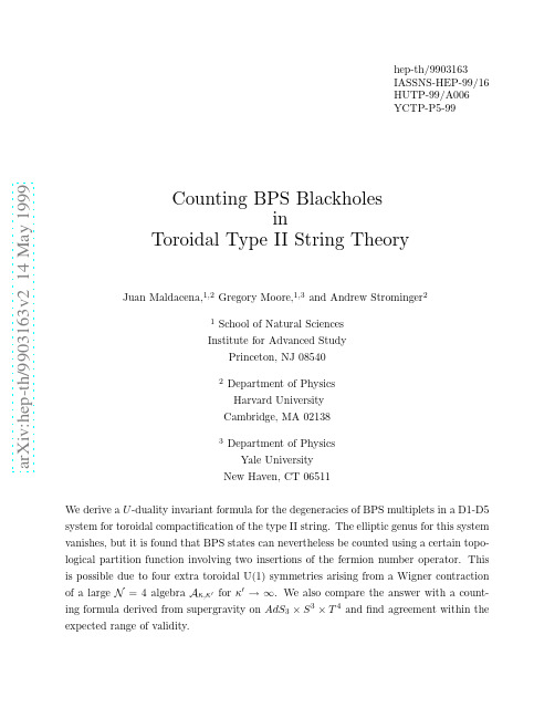
a r X i v :0905.2666v 2 [p h y s i c s .s o c -p h ] 23 J u l 2009APS/123-QEDQuantifying and identifying the overlapping community structure in networksHua-Wei Shen,∗Xue-Qi Cheng,†and Jia-Feng Guo ‡Institute of Computing Technology,Chinese Academy of Sciences,Beijing,ChinaIt has been shown that the communities of complex networks often overlap with each other.How-ever,there is no effective method to quantify the overlapping community structure.In this paper,we propose a metric to address this problem.Instead of assuming that one node can only belong to one community,our metric assumes that a maximal clique only belongs to one community.In this way,the overlaps between communities are allowed.To identify the overlapping community structure,we construct a maximal clique network from the original network,and prove that the optimization of our metric on the original network is equivalent to the optimization of Newman’s modularity on the maximal clique network.Thus the overlapping community structure can be iden-tified through partitioning the maximal clique network using any modularity optimization method.The effectiveness of our metric is demonstrated by extensive tests on both the artificial networks and the real world networks with known community structure.The application to the word association network also reproduces excellent results.PACS numbers:89.75.Fb,89.75.HcI.INTRODUCTIONMany complex systems in nature and society can be described in terms of networks or graphs.The study of networks is crucial to understand both the structure and the function of these complex systems [1,2].A common feature of complex networks is community structure,i.e.,the existence of groups of nodes such that nodes within a group are much more connected to each other than to the rest of the munities reflect the locality of the topological relationships between the elements of the target systems [3],and may shed light on the relation between the structure and the function of complex net-works.Take the World Wide Web as an example,closely hyperlinked web pages form a community and they often talk about related topics [4].The identification of community structure has at-tracted much attention from various scientific fields.Many methods have been proposed and applied success-fully to some specific complex networks [5,6,7,8,9,10,11,12,13,14].In order to quantify the commu-nity structure of networks,Newman and Girvan [6]pro-posed the modularity as a measure of a partition of net-work,in which each node only belongs to one commu-nity.The proposal of modularity has prompted the de-tection of community structure.However,the modular-ity faces several problems.For example,the modularity suffers a resolution limit problem [15,16].Furthermore,the modularity-based methods cannot tackle overlapping community structure,in which one node may belong to more than one community.Figure 1shows anexample2clique.However,the k-clique method gives rise to an uncomplete cover of network,i.e.,some nodes may not belong to any community.In addition,the hierarchical structure can not be revealed for a given k.In[24],by introducing the concept of the belonging coefficients of each node to its communities,the authors proposed a general framework for extending the traditional modu-larity to quantify overlapping community structure.The method provides a new idea tofind overlapping commu-nity structure.However,the physical meaning of the belonging coefficient lacks a clear explanation.Further-more,the framework is hard to extend to large scale net-works since it is difficult tofind an efficient algorithm to search the huge solution space.Recently,Evans et al[25] proposed a method to identify the overlapping commu-nity structure by partitioning a line graph constructed from the original network.This method only allows the communities to overlap at nodes.In this paper,a measure for the quality of a cover is proposed to quantify the overlapping community struc-ture referred as Q c(quality of a cover).With the measure Q c,the overlapping community structure can be identi-fied byfinding an optimal cover,i.e.,the one with the maximum Q c.The Q c is based on a maximal clique view of the original network.A maximal clique is a clique(i.e.a complete subgraph)which is not a subset of any other clique in a graph.The maximal clique view is accord-ing to a reasonable assumption that a maximal clique cannot be shared by two communities due to that it is highly connective.Tofind an optimal cover,we con-struct a maximal clique network from the original net-work.We then prove that the optimization of Q c on the original network is equivalent to the optimization of the modularity on the maximal clique network.Thus the overlapping community structure can be identified through partitioning the maximal clique network with an efficient modularity optimization algorithm,e.g.,the fast unfolding algorithm in[14].The effectiveness of the measure Q c is demonstrated by extensive tests on both the artificial networks and the real world networks with known community structure and the application to the word association network.II.THE QUANTIFYING AND IDENTIFYINGMETHODSIn this section,wefirst propose a measure Q c to quan-tify the overlapping community structure of networks. Then the overlapping community structure of a network is identified by partitioning a maximal clique network constructed from the original network using a modularity optimization algorithm.Finally,some discussions about our method are given.A.Quantifying the overlapping communitystructureAs mentioned above,the overlapping community struc-ture can be represented as a cover of network instead of a partition of network.Therefore,the overlapping com-munity structure can be quantified through a measure of a cover of network.As well known,the modularity was used to measure the goodness of a partition of network.Given an un-weighted,undirected network G(E,V)and a partition P of the network G,the modularity can be formalized as Q=1L ,(1)where A is the adjacency matrix of the network G,L= vw A vw is the total weight of all the edges,and k v= w A vw is the degree of the vertex v.In equation(1),δvc denotes whether the vertex v be-longs to the community c.The value ofδvc is1when the vertex v belongs to the community c and0otherwise.For a cover of network,however,a vertex may belong to more than one community.Thusδvc needs to be extended to a belonging coefficientαvc,which reflects how much the vertex v belongs to the community c.With the belonging coefficientαvc,the goodness of a cover C can be measured byQ c=1L .(2)The idea of the belonging coefficient was proposed in[24].Its authors also pointed out that the belonging coefficient should satisfy a normalization property.This property is formally written as0≤αvc≤1,∀v∈V,∀c∈C(3) andc∈Cαvc=1.(4)Equation(3)and equation(4)only give the general constraints onαvc,which lead to such a huge solution space that the enumeration of all the solutions is imprac-tical.To reduce the solution space and make the problem tractable,we introduce an additivity property for the be-longing coefficient:the belonging coefficient of a vertex to a community c is the sum of the belonging coefficients of the vertex to all of c’s sub-communities.For example,we assume that C={c1,c2,...,c r−1, c r,...,c s,c s+1,...,c n}is a cover of the network G and C′={c1,c2,...,c r−1,c u,c s+1,...,c n}is another cover of G.The difference between C′and C is that the com-munity c u is the union of the communities c r,...,c s.The additivity property of belonging coefficient can then beformally denoted asαvcu =si=rαvc i.(5)The belonging coefficientαvc reflects how much a ver-tex v belongs to a community c.Intuitively,it is pro-portional to the total weight of the edges connecting the vertex v to the vertices in the community c,i.e.,αvc∝ w∈V(c)A vw,(6)where V(c)denotes the set of vertices belonging to com-munity c.Note that the additivity property of belonging coefficient requires that communities are disjoint from a proper view of the network.Therefore,we introduce the maximal clique view to achieve this purpose.We define αvc as the formαvc=1O vwA vw,(7)where O vw denotes the number of maximal cliques con-taining the edge(v,w)in the whole network,O c vw denotes the number of maximal cliques containing the edge(v,w) in the community c,andαv is a normalization term de-noted asαv= c∈C w∈V(c)O cvw(d)All the maximal cliques:a: {1,2,4}All the subordinate vertices:d:{5}c: {7,8,9,10}b: {1,3,4}f: {11}e: {6}(b) A cover of the original networkFIG.2:Illustration for the construction process of the maximal clique network.(a)The original example network.(b)A cover of the original network.In this cover,each maximal clique is a cluster and each subordinate vertex forms a cluster consisting of only one vertex.(c)The belonging coefficient of each vertex to its corresponding clusters in the cover.(d)The maximal clique network constructed from the example network.Here the parameter k =3.and the node b corresponds to the maximal clique {1,3,4}.Using the equation (9),the weight of this edge is α1a α3b +α1a α4b +α2a α1b +α2a α4b +α4a α1b +α4a α3b =0.5+0.25+0.5+0.5+0.25+0.5=2.5.The constructed maximal clique network is a weighted network though the original network is un-weighted.The total weight L ′of all the edges in the maximal clique network is equal to the total weight (number)L of edges in the original network.The proof isL ′=xyB xy= xy vwαvm x αwm y A vw =vw A vwxαvm xyαwm y=vw A vw=L.(11)Each vertex in the original network corresponds to more than one node in the maximal clique network.For example,in figure 2,the vertex 1corresponds to two nodes a and b in the maximal clique network.Thus,a partition of the maximal clique network can be mapped to a cover of the original network,which holds the in-formation about the overlapping community structure of the original network.2.Finding the overlapping community structureNow we investigate the overlapping community struc-ture of the original network through partitioning its cor-responding maximal clique network.To find the natural partition of a network,the optimization of modularity is the widely used technique.The partition with the max-imum modularity is regarded as the optimal partition of network.We employ the algorithm proposed in [14]to partition our maximal clique network.As an exam-ple,figure 3shows the partition of a maximal clique net-work.Different parts of the partition are differentiated by shapes or colors.As mentioned above,each partition of the maximal clique network corresponds to a cover of the original net-work and the cover tells us the overlapping community structure.The key problem lies in that whether the opti-mal partition of the maximal clique network corresponds to the optimal cover of the original network.To answer this question,we analyze the relation between the mod-ularity of the maximal clique network and the Q c of the original network.Let P ={p 1,p 2,...,p l }be a partition of the maximal clique network and C ={c 1,c 2,...,c l }be the correspond-ing cover of the original network.Here,l is the size of P or C ,i.e.,the number of ing modularity,the quality of the partition P can be measured byQ =1L ′.(12)5FIG.3:The maximal clique network constructed from theschematic network infigure1.The label near each node showsits corresponding vertices in the original network.The widthof line indicates the weight of the corresponding edge.Theself-loop edge of each node is omitted and its width is reflectedby the volume of the associated circles,squares or triangles.Inaddition,the optimal partition of the maximal clique networkis also depicted.The communities in this partition are differ-entiated by shapes.Furthermore,the circle-coded communitycan be partitioned into two sub-communities.The four com-munities are shown in different colors,which are identical tothe communities depicted infigure1.Here k is4.Using equations(9)and(10),we haveQ=1L′ vαvm x k v wαwm y k w=1L′=1L=Q c.(13) Equation(13)tells us that the optimization of the Q c on the original network is equivalent to the optimization of the modularity on the maximal clique network.Thus we canfind the optimal cover of the original network by finding the optimal partition of the corresponding maxi-mal clique network.The optimal cover reflects the over-lapping community structure of the original network.C.DiscussionsAs to our method,it is important to select an appro-priate parameter k.On one hand,the parameter k af-fects the constituent of the overlapping regions between communities.According to the definition to subordinate vertices,they are excluded from the overlapping regions.Thus the larger the parameter k,the less the number of vertices which can occur in the overlapping regions. When k→∞,the maximal clique network is identical to the original network and no overlap is identified.On the other hand,since the subordinate maximal cliques are not so highly connective,the parameter k should not be too small in practice.The choice of the parameter k depends on the specific networks.Observed from many real world networks,the typical value of k is often be-tween3and6.Additionally,as to the networks where larger cliques are rare,our method is close to the tradi-tional modularity-based partition methods.In this case, rare overlaps will be found.Both the traditional modularity and the Q c are based on the significance of link density in communities com-pared to a null-model reference network,e.g.,the con-figuration model network.However,differently from the traditional modularity which requires that each node can only belong to one community,Q c requires that each maximal clique can only belong to one community.In this way,Q c takes advantage of both the local topolog-ical structure(i.e.,the maximal clique)and the global statistical significance of link density.The same to the traditional modularity,however,the measure Q c also suffers the resolution limit problem[15], especially when applied to large scale complex networks. Recently,some methods[26]have been proposed to ad-dress the resolution limit problem of modularity.These methods are also appropriate to the measure Q c.Now we turn to the efficiency of our method.It is difficult to give an analytical form of the computational complexity of our method.Here we only discuss what in-fluences the efficiency of our method.Our method con-sists of three stages,finding out the maximal cliques, constructing the maximal clique network and partition-ing the maximal clique network.As to thefirst stage, we need tofind out all the maximal cliques in the net-work.It is widely believed to be a non-polynomial prob-lem.However,for real world networks,finding all the maximal cliques is easy due to the sparseness of these networks.The computational complexity of the second stage depends on the number of edges in the original net-works.Finally,the partition stage rests with the number of the maximal cliques and subordinate vertices.Taken together,our method is very efficient on real world net-works.In addition,as mentioned above,the overlapping com-munity structure can be identified by the optimization of Q c.Similarly,iteratively applying this method to each community,we can investigate the sub-communities cor-respondingly.In this way,a rigid hierarchical relation of overlapping communities can be identified from the whole network.6FIG.4:Test of our method on the benchmark networks.The parameter k in the legend corresponds to the parameter k in our method.The thresholdµ=0.5(dashed vertical line in thefigure)marks the borderbeyond which communities are no longer defined in the strong sense[28],i.e.,such that each node has more neighbors in its own community than in the others.Each point corresponds to an average over100graph realization.III.RESULTSIn this section,we extensively test our method on the artificial networks and the real world networks with known community structure.Then we apply our method to a large real world complex network,which has been shown to possess overlapping community structure.A.Tests on artificial networksTo test our method,we utilize the benchmark proposed in[27].It provides benchmark networks with heteroge-nous distributions of node degree and community size.In addition,it allows for the overlaps between communities. This benchmark poses a much more severe test to com-munity detection algorithms than Newman’s standard benchmark[6].There are many parameters to control the generated networks in this benchmark,the number of nodes N,the average node degree k ,the maximum node degree maxk,the mixing ratioµ,the exponent of the power-law node degree distribution t1,the exponent of the power-law distribution of community size t2,the minimum community size minc,the maximum commu-nity size maxc,the number of overlapped nodes on,and the number of memberships of each overlapped node om. In our tests,we use the default parameter configuration where N=1000, k =15,maxk=50,t1=2,t2=1, mic=20,maxc=50,on=50and om=2.By tuning the parameterµ,we test the effectiveness of our method on the networks with different fuzziness of communities. The larger the parameterµ,the fuzzier the community FIG.5:The network of the karate club studied by Zachary[29].The real socialfission of this network is rep-resented by two different shapes,circle and square.The dif-ferent colors show the partition obtained by our method with the parameter k=4.structure of the generated networks is.To evaluate the effectiveness of an algorithm for the identification of overlapping community structure,a mea-sure is needed to compare the cover found by the algo-rithm with the ground truth.In[23],a measure is pro-posed to compare two covers,which is an extension form of variation of information.The more similar two covers are,the higher the value of the measure is.In this pa-per,we adopt it to compare the overlapping community structure found by our method and the known overlap-ping community structure in the benchmark networks. Figure4shows the results of our method with k= 4,5,6on the benchmark networks.Our method gives rather good results when theµis smaller than0.5.All of the values of the variation of information are above0.8. Note that in these cases,communities are defined in the strong sense[28],i.e.,each node has more neighbors in its own community than in the others.We also test other settings of k which are larger than6,andfind similar results.B.Tests on real world networksOurfirst real world network for test is Zachary’s karate club network[29],which is widely used as a benchmark for the methods of community identification.This net-work characterizes the social interactions between the in-dividuals in a karate club at an American university.A dispute arose between the club’s administrator and its principal karate teacher and as a result the club even-tually split into two smaller clubs,centered around the administrator and the teacher respectively.The network and itsfission is depicted infigure5.The administra-tor and the teacher are represented by nodes1and33 respectively.Feeding this network into our method with the pa-rameter k=4,we obtain the result shown infigure5. Similar to many existing community detection methods, our method partitions the network into four communi-FIG.6:The community structure identified by our method from the network of the bottlenose dolphins of Doubtful Sound. The primary split of the network is represented by different shapes,square and circle.The different colors show the partition obtained by our method with the parameter k=4.ties.This partition corresponds to the modularity with the value0.417,while the real partition into two sub-networks has a modularity0.371.Actually,no vertex is misclassified by our method.The real split of the net-work can be obtained exactly by pair-wise merge of the four communities found by our method.We also note that no overlaps are found when k=4. Actually,no overlaps can be found when k is no smaller than4as to this network.Overlaps between communi-ties emerge when the parameter k is set to3.The value of Q c corresponding to the resulting cover is0.385and in total three overlapped communities are found by our method.They are{1,5,6,7,11,17},{1,2,3,4,8,9,12, 13,14,18,20,22}and{3,9,10,15,16,19,21,23,24, 25,26,27,28,29,30,31,32,33,34}.The overlapping regions consist of three vertices,being1,3and9.Each of them is shared by two communities.Such vertices are often misclassified by traditional partition-based commu-nity detection methods.Except the vertices occurring in the overlapping regions,other vertices reflects the real split of the network.We also test our method on another real world net-work,a social network of62bottlenose dolphins living in Doubtful Sound,New Zealand.The network was con-structed by Lusseau[30]with ties between dolphin pairs being established by observation of statistically signifi-cant frequent association.The network splits naturally into two groups,represented by the squares and circles infigure6.By applying our method with k=4to this network, four communities are obtained,denoted by different col-ors infigure6.The green community is connected loosely to the other three ones.Regarding the three circle-denoted communities as a sole community,it and the green community correspond to the known division ob-served by Lusseau[30].Furthermore,the three circle-denoted communities also correspond to a real division among these dolphins.The further division appears to have some correlation with the gender of these animals. The blue one consists mainly of females and the other two almost entirely of males.Alike to the Zarchay’s karate network,the overlaps be-tween communities cannot be detected when the param-eter k is not less than4.When k=3,overlaps between the circle-denoted communities emerge while the green community keeps almost intact.The Q c is0.490as to the resulting cover.The vertices occurring in overlap-ping regions are Beak,Kringel,MN105,Oscar,P L, SN4,SN9and T R99among which the vertices Beak and Kringel are shared by all the three circle-denoted communities.Again these overlapping vertices are often misclassified by traditional partition-based methods. C.Application to the word association networkNow we apply our method to a large real world complex network,namely the word association network.The data set for the word association network is from the demo of the software CFinder[31].This network consists of7207vertices and31784edges,and has been shown to possess overlapping community structure[17]. It is constructed from the South Florida Free Associa-tion norms list[32].Initially,the network is a directed, weighted network.The weight of a directed edge from one word to another indicates the frequency that theTABLE I:The overlapping communities around the word play.For each community,a short description is also given.The overlapped words are emphasized in bold texts.Description1act actor actress bow character cinema curtsey dance director do drama entertain entertainmentfilm guide involve juggler lead movie participate perform performance play portray producer production programscene screen show sing stage television theatermusicalinstrument3adults balls children family friends fun grown-ups guardians kids love mischief nursery parents play play-ground play4active arena athlete athletic baseball basketball black whitefield football fun game illustrated inactive jock pigskin play recreation referee soccer sports stadium umpiretoysyooptimization method on the maximal clique network. The Q c is an extension of traditional modularity with the consideration that the maximal clique instead of a single node can only belong to one community.In this way,Q c takes advantage of both the local topological structure(i.e.,the maximal clique)and the global sta-tistical significance of link density compared with a null-model reference network.In addition,Q c can be nat-urally used to simultaneously identify the overlapping and hierarchical community structure of networks.Such a method is helpful to more completely understand the functional and structural properties of networks.As the further work,we will consider the generalization to the weighted and/or directed networks.It is also an interesting problem about the selection of the parameter k in our method.We will further investigate how to determine an appropriate k for a given network later.AcknowledgmentsThis work was funded by the National Natural Sci-ence Foundation of China under grant number60873245, the National High-Tech R&D Program of China(the863 program)under grant number2006AA01Z452,and the National Basic Research Program of China(the973pro-gram)under grant number2004CB318109.The authors gratefully acknowledge S.Fortunato and ncichinetti for providing the test benchmark and useful discussions on it.The authors thank Mao-Bin Hu for helpful sugges-tions.[1]Albert R and Barab´a si A-L,2002Rev.Mod.Phys.7447[2]Newman M E J,2003SIAM Rev.45167[3]Cheng X Q,Ren F X,Zhou S and Hu M B,2009,NewJ.Phys.11033019[4]Flake G W,Lawrence S,Giles C L and Coetzee F M,2002IEEE Comput.3566[5]Girvan M and Newman M E J,2002Proc.Natl.Acad.A997821[6]Newman M E J and Girvan M,2004Phys.Rev.E69026113[7]Newman M E J,2004Phys.Rev.E69066133[8]Clauset A,Newman M E J and Moore C,2004Phys.Rev.E70066111[9]Guimer`a R and Amaral L A N,2005Nature433895[10]Duch J and Arenas A,2005Phys.Rev.E72027104[11]Newman M E J,A1038577[12]Raghavan U N,Albert R and Kumara S,2007Phys.Rev.E76036106[13]Sales-Pardo M,Guimer`a R,Moreira A A and Amaral LA N,A10415224[14]Blondel V D,Guillaume J-L,Lambiotte R and LefebvreE,2008J.Stat.Mech.P10008[15]Fortunato S and Barth´e lemy M,2007Proc.Natl.Acad.A10436[16]Kumpula J M,Saramaki J,Kaski K and Kertesz J,2007Eur.Phys.J.B5641[17]Palla G,Der´e nyi I,Farkas I and Vicsek T,2005Nature435814[18]Baumes J,Goldberg M K,Krishnamoorthy M S,Magdon-Ismail M and Preston N,2005Proc.IADIS Ap-plied Computing97[19]Zhang S,Wang R S and Zhang X S,2007Physica A374483[20]Palla G,Farkas I J,Pollner P,Der´e nyi I and Vicsek T,2007New J.Phys.9186[21]Farkas I J,´Abel D,Palla G and Vicsek T,2007New J.Phys.9180[22]Shen H W,Cheng X Q,Cai K and Hu M B,2009PhysicaA3881706[23]Lancichinetti A,Fortunato S and Kert´e sz J,2009New J.Phys.11033015[24]Nicosia V,Mangioni G,Carchiolo V and Malgeri M,2009J.Stat.Mech.P03024[25]Evans T S and Lambiotte R,2009arXiv:0903.2181[26]Arenas A,Fern´a ndez A and G´o mez S,2008New J.Phys.10053039[27]Lancichinetti A and Fortunato S,2009arXiv:0904:3940[28]Radicchi F,Castellano C,Cecconi F,Loreto V and ParisiD,A1012658[29]Zachary W W,1977J.Anthropol.33452[30]Lusseau D,Schneider K,Boisseau O J,Haase P,SlootenE and Dawson S M,2003Behav.Ecol.Sociobiol.54396[31]Adamcsek B,Palla G,Farkas I J,Der´e nyi I and VicsekT,2006Bioinformatics221021[32]Nelson D L,McEvoy C L and Schreiber T A,1998/FreeAssociation/。

a r X i v :c o n d -m a t /9503139v 1 27 M a r 1995Singularity of the density of states in the two-dimensional Hubbard model from finitesize scaling of Yang-Lee zerosE.Abraham 1,I.M.Barbour 2,P.H.Cullen 1,E.G.Klepfish 3,E.R.Pike 3and Sarben Sarkar 31Department of Physics,Heriot-Watt University,Edinburgh EH144AS,UK 2Department of Physics,University of Glasgow,Glasgow G128QQ,UK 3Department of Physics,King’s College London,London WC2R 2LS,UK(February 6,2008)A finite size scaling is applied to the Yang-Lee zeros of the grand canonical partition function for the 2-D Hubbard model in the complex chemical potential plane.The logarithmic scaling of the imaginary part of the zeros with the system size indicates a singular dependence of the carrier density on the chemical potential.Our analysis points to a second-order phase transition with critical exponent 12±1transition controlled by the chemical potential.As in order-disorder transitions,one would expect a symmetry breaking signalled by an order parameter.In this model,the particle-hole symmetry is broken by introducing an “external field”which causes the particle density to be-come non-zero.Furthermore,the possibility of the free energy having a singularity at some finite value of the chemical potential is not excluded:in fact it can be a transition indicated by a divergence of the correlation length.A singularity of the free energy at finite “exter-nal field”was found in finite-temperature lattice QCD by using theYang-Leeanalysisforthechiral phase tran-sition [14].A possible scenario for such a transition at finite chemical potential,is one in which the particle den-sity consists of two components derived from the regular and singular parts of the free energy.Since we are dealing with a grand canonical ensemble,the particle number can be calculated for a given chem-ical potential as opposed to constraining the chemical potential by a fixed particle number.Hence the chem-ical potential can be thought of as an external field for exploring the behaviour of the free energy.From the mi-croscopic point of view,the critical values of the chemical potential are associated with singularities of the density of states.Transitions related to the singularity of the density of states are known as Lifshitz transitions [15].In metals these transitions only take place at zero tem-perature,while at finite temperatures the singularities are rounded.However,for a small ratio of temperature to the deviation from the critical values of the chemical potential,the singularity can be traced even at finite tem-perature.Lifshitz transitions may result from topological changes of the Fermi surface,and may occur inside the Brillouin zone as well as on its boundaries [16].In the case of strongly correlated electron systems the shape of the Fermi surface is indeed affected,which in turn may lead to an extension of the Lifshitz-type singularities into the finite-temperature regime.In relating the macroscopic quantity of the carrier den-sity to the density of quasiparticle states,we assumed the validity of a single particle excitation picture.Whether strong correlations completely distort this description is beyond the scope of the current study.However,the iden-tification of the criticality using the Yang-Lee analysis,remains valid even if collective excitations prevail.The paper is organised as follows.In Section 2we out-line the essentials of the computational technique used to simulate the grand canonical partition function and present its expansion as a polynomial in the fugacity vari-able.In Section 3we present the Yang-Lee zeros of the partition function calculated on 62–102lattices and high-light their qualitative differences from the 42lattice.In Section 4we analyse the finite size scaling of the Yang-Lee zeros and compare it to the real-space renormaliza-tion group prediction for a second-order phase transition.Finally,in Section 5we present a summary of our resultsand an outlook for future work.II.SIMULATION ALGORITHM AND FUGACITY EXPANSION OF THE GRAND CANONICALPARTITION FUNCTIONThe model we are studying in this work is a two-dimensional single-band Hubbard HamiltonianˆH=−t <i,j>,σc †i,σc j,σ+U i n i +−12 −µi(n i ++n i −)(1)where the i,j denote the nearest neighbour spatial lat-tice sites,σis the spin degree of freedom and n iσis theelectron number operator c †iσc iσ.The constants t and U correspond to the hopping parameter and the on-site Coulomb repulsion respectively.The chemical potential µis introduced such that µ=0corresponds to half-filling,i.e.the actual chemical potential is shifted from µto µ−U412.(5)This transformation enables one to integrate out the fermionic degrees of freedom and the resulting partition function is written as an ensemble average of a product of two determinantsZ ={s i,l =±1}˜z = {s i,l =±1}det(M +)det(M −)(6)such thatM ±=I +P ± =I +n τ l =1B ±l(7)where the matrices B ±l are defined asB ±l =e −(±dtV )e −dtK e dtµ(8)with V ij =δij s i,l and K ij =1if i,j are nearestneigh-boursand Kij=0otherwise.The matrices in (7)and (8)are of size (n x n y )×(n x n y ),corresponding to the spatial size of the lattice.The expectation value of a physical observable at chemical potential µ,<O >µ,is given by<O >µ=O ˜z (µ){s i,l =±1}˜z (µ,{s i,l })(9)where the sum over the configurations of Ising fields isdenoted by an integral.Since ˜z (µ)is not positive definite for Re(µ)=0we weight the ensemble of configurations by the absolute value of ˜z (µ)at some µ=µ0.Thus<O >µ= O ˜z (µ)˜z (µ)|˜z (µ0)|µ0|˜z (µ0)|µ0(10)The partition function Z (µ)is given byZ (µ)∝˜z (µ)N c˜z (µ0)|˜z (µ0)|×e µβ+e −µβ−e µ0β−e −µ0βn (16)When the average sign is near unity,it is safe to as-sume that the lattice configurations reflect accurately thequantum degrees of freedom.Following Blankenbecler et al.[1]the diagonal matrix elements of the equal-time Green’s operator G ±=(I +P ±)−1accurately describe the fermion density on a given configuration.In this regime the adiabatic approximation,which is the basis of the finite-temperature algorithm,is valid.The situa-tion differs strongly when the average sign becomes small.We are in this case sampling positive and negative ˜z (µ0)configurations with almost equal probability since the ac-ceptance criterion depends only on the absolute value of ˜z (µ0).In the simulations of the HSfields the situation is dif-ferent from the case of fermions interacting with dynam-ical bosonfields presented in Ref.[1].The auxilary HS fields do not have a kinetic energy term in the bosonic action which would suppress their rapidfluctuations and hence recover the adiabaticity.From the previous sim-ulations on a42lattice[3]we know that avoiding the sign problem,by updating at half-filling,results in high uncontrolledfluctuations of the expansion coefficients for the statistical weight,thus severely limiting the range of validity of the expansion.It is therefore important to obtain the partition function for the widest range ofµ0 and observe the persistence of the hierarchy of the ex-pansion coefficients of Z.An error analysis is required to establish the Gaussian distribution of the simulated observables.We present in the following section results of the bootstrap analysis[17]performed on our data for several values ofµ0.III.TEMPERATURE AND LATTICE-SIZEDEPENDENCE OF THE YANG-LEE ZEROS The simulations were performed in the intermediate on-site repulsion regime U=4t forβ=5,6,7.5on lat-tices42,62,82and forβ=5,6on a102lattice.The ex-pansion coefficients given by eqn.(14)are obtained with relatively small errors and exhibit clear Gaussian distri-bution over the ensemble.This behaviour was recorded for a wide range ofµ0which makes our simulations reli-able in spite of the sign problem.In Fig.1(a-c)we present typical distributions of thefirst coefficients correspond-ing to n=1−7in eqn.(14)(normalized with respect to the zeroth power coefficient)forβ=5−7.5for differ-entµ0.The coefficients are obtained using the bootstrap method on over10000configurations forβ=5increasing to over30000forβ=7.5.In spite of different values of the average sign in these simulations,the coefficients of the expansion(16)indicate good correspondence between coefficients obtained with different values of the update chemical potentialµ0:the normalized coefficients taken from differentµ0values and equal power of the expansion variable correspond within the statistical error estimated using the bootstrap analysis.(To compare these coeffi-cients we had to shift the expansion by2coshµ0β.)We also performed a bootstrap analysis of the zeros in theµplane which shows clear Gaussian distribution of their real and imaginary parts(see Fig.2).In addition, we observe overlapping results(i.e.same zeros)obtained with different values ofµ0.The distribution of Yang-Lee zeros in the complexµ-plane is presented in Fig.3(a-c)for the zeros nearest to the real axis.We observe a gradual decrease of the imaginary part as the lattice size increases.The quantitative analysis of this behaviour is discussed in the next section.The critical domain can be identified by the behaviour of the density of Yang-Lee zeros’in the positive half-plane of the fugacity.We expect tofind that this density is tem-perature and volume dependent as the system approaches the phase transition.If the temperature is much higher than the critical temperature,the zeros stay far from the positive real axis as it happens in the high-temperature limit of the one-dimensional Ising model(T c=0)in which,forβ=0,the points of singularity of the free energy lie at fugacity value−1.As the temperature de-creases we expect the zeros to migrate to the positive half-plane with their density,in this region,increasing with the system’s volume.Figures4(a-c)show the number N(θ)of zeros in the sector(0,θ)as a function of the angleθ.The zeros shown in thesefigures are those presented in Fig.3(a-c)in the chemical potential plane with other zeros lying further from the positive real half-axis added in.We included only the zeros having absolute value less than one which we are able to do because if y i is a zero in the fugacity plane,so is1/y i.The errors are shown where they were estimated using the bootstrap analysis(see Fig.2).Forβ=5,even for the largest simulated lattice102, all the zeros are in the negative half-plane.We notice a gradual movement of the pattern of the zeros towards the smallerθvalues with an increasing density of the zeros nearθ=πIV.FINITE SIZE SCALING AND THESINGULARITY OF THE DENSITY OF STATESAs a starting point for thefinite size analysis of theYang-Lee singularities we recall the scaling hypothesis forthe partition function singularities in the critical domain[11].Following this hypothesis,for a change of scale ofthe linear dimension LLL→−1),˜µ=(1−µT cδ(23)Following the real-space renormalization group treatmentof Ref.[11]and assuming that the change of scaleλisa continuous parameter,the exponentαθis related tothe critical exponentνof the correlation length asαθ=1ξ(θλ)=ξ(θ)αθwe obtain ξ∼|θ|−1|θ|ναµ)(26)where θλhas been scaled to ±1and ˜µλexpressed in terms of ˜µand θ.Differentiating this equation with respect to ˜µyields:<n >sing =(−θ)ν(d −αµ)∂F sing (X,Y )ν(d −αµ)singinto the ar-gument Y =˜µαµ(28)which defines the critical exponent 1αµin terms of the scaling exponent αµof the Yang-Lee zeros.Fig.5presents the scaling of the imaginary part of the µzeros for different values of the temperature.The linear regression slope of the logarithm of the imaginary part of the zeros plotted against the logarithm of the inverse lin-ear dimension of the simulation volume,increases when the temperature decreases from β=5to β=6.The re-sults of β=7.5correspond to αµ=1.3within the errors of the zeros as the simulation volume increases from 62to 82.As it is seen from Fig.3,we can trace zeros with similar real part (Re (µ1)≈0.7which is also consistentwith the critical value of the chemical potential given in Ref.[22])as the lattice size increases,which allows us to examine only the scaling of the imaginary part.Table 1presents the values of αµand 1αµδ0.5±0.0560.5±0.21.3±0.3∂µ,as a function ofthe chemical potential on an 82lattice.The location of the peaks of the susceptibility,rounded by the finite size effects,is in good agreement with the distribution of the real part of the Yang-Lee zeros in the complex µ-plane (see Fig.3)which is particularly evident in the β=7.5simulations (Fig.4(c)).The contribution of each zero to the susceptibility can be singled out by expressing the free energy as:F =2n x n yi =1(y −y i )(29)where y is the fugacity variable and y i is the correspond-ing zero of the partition function.The dotted lines on these plots correspond to the contribution of the nearby zeros while the full polynomial contribution is given by the solid lines.We see that the developing singularities are indeed governed by the zeros closest to the real axis.The sharpening of the singularity as the temperature de-creases is also in accordance with the dependence of the distribution of the zeros on the temperature.The singularities of the free energy and its derivative with respect to the chemical potential,can be related to the quasiparticle density of states.To do this we assume that single particle excitations accurately represent the spectrum of the system.The relationship between the average particle density and the density of states ρ(ω)is given by<n >=∞dω1dµ=ρsing (µ)∝1δ−1(32)and hence the rate of divergence of the density of states.As in the case of Lifshitz transitions the singularity of the particle number is rounded at finite temperature.However,for sufficiently low temperatures,the singular-ity of the density of states remains manifest in the free energy,the average particle density,and particle suscep-tibility [15].The regular part of the density of states does not contribute to the criticality,so we can concentrate on the singular part only.Consider a behaviour of the typedensity of states diverging as the−1ρsing(ω)∝(ω−µc)1δ.(33)with the valueδfor the particle number governed by thedivergence of the density of states(at low temperatures)in spite of thefinite-temperature rounding of the singu-larity itself.This rounding of the singularity is indeedreflected in the difference between the values ofαµatβ=5andβ=6.V.DISCUSSION AND OUTLOOKWe note that in ourfinite size scaling analysis we donot include logarithmic corrections.In particular,thesecorrections may prove significant when taking into ac-count the fact that we are dealing with a two-dimensionalsystem in which the pattern of the phase transition islikely to be of Kosterlitz-Thouless type[23].The loga-rithmic corrections to the scaling laws have been provenessential in a recent work of Kenna and Irving[24].In-clusion of these corrections would allow us to obtain thecritical exponents with higher accuracy.However,suchanalysis would require simulations on even larger lattices.The linearfits for the logarithmic scaling and the criti-cal exponents obtained,are to be viewed as approximatevalues reflecting the general behaviour of the Yang-Leezeros as the temperature and lattice size are varied.Al-though the bootstrap analysis provided us with accurateestimates of the statistical error on the values of the ex-pansion coefficients and the Yang-Lee zeros,the smallnumber of zeros obtained with sufficient accuracy doesnot allow us to claim higher precision for the critical ex-ponents on the basis of more elaboratefittings of the scal-ing behaviour.Thefinite-size effects may still be signifi-cant,especially as the simulation temperature decreases,thus affecting the scaling of the Yang-Lee zeros with thesystem rger lattice simulations will therefore berequired for an accurate evaluation of the critical expo-nent for the particle density and the density of states.Nevertheless,the onset of a singularity atfinite temper-ature,and its persistence as the lattice size increases,areevident.The estimate of the critical exponent for the diver-gence rate of the density of states of the quasiparticleexcitation spectrum is particularly relevant to the highT c superconductivity scenario based on the van Hove sin-gularities[25],[26],[27].It is emphasized in Ref.[25]thatthe logarithmic singularity of a two-dimensional electrongas can,due to electronic correlations,turn into a power-law divergence resulting in an extended saddle point atthe lattice momenta(π,0)and(0,π).In the case of the14.I.M.Barbour,A.J.Bell and E.G.Klepfish,Nucl.Phys.B389,285(1993).15.I.M.Lifshitz,JETP38,1569(1960).16.A.A.Abrikosov,Fundamentals of the Theory ofMetals North-Holland(1988).17.P.Hall,The Bootstrap and Edgeworth expansion,Springer(1992).18.S.R.White et al.,Phys.Rev.B40,506(1989).19.J.E.Hirsch,Phys.Rev.B28,4059(1983).20.M.Suzuki,Prog.Theor.Phys.56,1454(1976).21.A.Moreo, D.Scalapino and E.Dagotto,Phys.Rev.B43,11442(1991).22.N.Furukawa and M.Imada,J.Phys.Soc.Japan61,3331(1992).23.J.Kosterlitz and D.Thouless,J.Phys.C6,1181(1973);J.Kosterlitz,J.Phys.C7,1046(1974).24.R.Kenna and A.C.Irving,unpublished.25.K.Gofron et al.,Phys.Rev.Lett.73,3302(1994).26.D.M.Newns,P.C.Pattnaik and C.C.Tsuei,Phys.Rev.B43,3075(1991);D.M.Newns et al.,Phys.Rev.Lett.24,1264(1992);D.M.Newns et al.,Phys.Rev.Lett.73,1264(1994).27.E.Dagotto,A.Nazarenko and A.Moreo,Phys.Rev.Lett.74,310(1995).28.A.A.Abrikosov,J.C.Campuzano and K.Gofron,Physica(Amsterdam)214C,73(1993).29.D.S.Dessau et al.,Phys.Rev.Lett.71,2781(1993);D.M.King et al.,Phys.Rev.Lett.73,3298(1994);P.Aebi et al.,Phys.Rev.Lett.72,2757(1994).30.E.Dagotto, A.Nazarenko and M.Boninsegni,Phys.Rev.Lett.73,728(1994).31.N.Bulut,D.J.Scalapino and S.R.White,Phys.Rev.Lett.73,748(1994).32.S.R.White,Phys.Rev.B44,4670(1991);M.Veki´c and S.R.White,Phys.Rev.B47,1160 (1993).33.C.E.Creffield,E.G.Klepfish,E.R.Pike and SarbenSarkar,unpublished.Figure CaptionsFigure1Bootstrap distribution of normalized coefficients for ex-pansion(14)at different update chemical potentialµ0for an82lattice.The corresponding power of expansion is indicated in the topfigure.(a)β=5,(b)β=6,(c)β=7.5.Figure2Bootstrap distributions for the Yang-Lee zeros in the complexµplane closest to the real axis.(a)102lat-tice atβ=5,(b)102lattice atβ=6,(c)82lattice at β=7.5.Figure3Yang-Lee zeros in the complexµplane closest to the real axis.(a)β=5,(b)β=6,(c)β=7.5.The correspond-ing lattice size is shown in the top right-hand corner. Figure4Angular distribution of the Yang-Lee zeros in the com-plex fugacity plane Error bars are drawn where esti-mated.(a)β=5,(b)β=6,(c)β=7.5.Figure5Scaling of the imaginary part ofµ1(Re(µ1)≈=0.7)as a function of lattice size.αm u indicates the thefit of the logarithmic scaling.Figure6Electronic susceptibility as a function of chemical poten-tial for an82lattice.The solid line represents the con-tribution of all the2n x n y zeros and the dotted line the contribution of the six zeros nearest to the real-µaxis.(a)β=5,(b)β=6,(c)β=7.5.。

Learning Based Super-Resolution Imaging:Use ofZoom as a CueB.Tech.Project ReportSubmitted in partial fulfillmentof the requirements forB.Tech.DegreeinElectrical EngineeringbyRajkiran Panuganti(99007034)under the guidance ofProf.Subhasis ChaudhuriDepartment of Electrical EngineeringIndian Institute of Technology,BombayApril20032Acceptance CertificateDepartment of Electrical EngineeringIndian Institute of Technology,BombayThe Bachelor of Technology project titled Learning Based Super-Resolution Imaging:Use of Zoom as a Cue and the corresponding report was done by Rajkiran Panuganti(99007034) under my guidance and may be accepted.Date:April16,2003(Prof.Subhasis Chaudhuri)AcknowledgmentI would like to express my sincere gratitude towards Prof.Subhasis Chaudhuri for his invaluable guidance and constant encouragement and Mr.Manjunath Joshi for his help during the course of the project.16th April,2003Rajkiran PanugantiAbstractWe propose a novel technique for super-resolution imaging of a scene from observations at different camera zooms.Given a sequence of images with different zoom factors of a static scene,the problem is to obtain a picture of the entire scene at a resolution corresponding to the most zoomed image in the scene.We not only obtain the super-resolved image for known integer zoom factors,but also for unknown arbitrary zoom factors.In order to achieve that we model the high resolution image as a Markov randomfield(MRF)the parameters of which are learnt from the most zoomed observation.The parameters are estimated using the maximum pseudo-likelihood(MPL)criterion.Assuming that the entire scene can be described by a homogeneous MRF,the learnt model parameters are then used to obtain a maximum aposteriori(MAP)estimate of the high resolutionfield.Since there is no relative motion between the scene and the camera,as is the case with most of the super-resolution techniques, we do away with the correspondence problem.Experimental results on synthetic as well as on real data sets are presented.ContentsAcceptance Certificate iAcknowledgment ii Abstract iii Table of Contents iv 1Introduction1 Introduction1 2Related Work4 Related Work4 3Low Resolution Image Model9 Low Resolution Image Model9 4Super-Resolution Restoration12Super-Resolution Resotoration124.1Image Field Modeling (12)4.2Parameter Learning (14)4.3MAP Restoration (15)4.4Zoom Estimation (16)5Experimental Results19Experimental Results195.1Experimentations with Known,Integer Zoom Factors (19)5.2Experiments with unknown zoom factors (25)5.3Experimental Results when parameters are estimated (28)6Conclusion33 Conclusion33 References34Chapter1IntroductionIn most electronic imaging applications,images with high spatial resolution are desired and often required.A high spatial resolution means that the pixel density in an image is high,and hence there are more details and subtle gray level transitions,which may be critical in various applications.Be it remote sensing,medical imaging,robot vision,industrial inspection or video enhancement(to name a few),operating on high-resolution images leads to a better analysis in the form of lesser misclassification,better fault detection,more true-positives,etc. However,acquisition of high-resolution images is severely constrained by the drawbacks of the limited density sensors.The images acquired through such sensors suffer from aliasing and blurring.The most direct solution to increase the spatial resolution is to reduce the pixel size (i.e.,to increase the number of pixels per unit area)by the sensor manufacturing techniques. But due to the decrease in pixel size,the light available also decreases causing more shot noise [1,2]which degrades the image quality.Thus,there exists limitations on the pixel size and the optimal size is estimated to be about40µm2.The current image sensor technology has almost reached this level.Another approach to increase the resolution is to increase the wafer size which leads to an increase in the capacitance[3].This approach is not effective since an increase in the capacitance causes a decrease in charge transfer rate.Hence,a promising approach is to use image processing methods to construct a high-resolution image from one or more available low-resolution observations.Resolution enhancement from a single observation using image interpolation techniquesis of limited application because of the aliasing present in the low-resolution image.Super-resolution refers to the process of producing a high spatial resolution image from several low-resolution observations.It includes upsampling the image thereby increasing the maximum spatial frequency and removing degradations that arise during image capture,viz.,aliasing and blurring.The amount of aliasing differs with zooming.This is because,when one captures the images with different zoom settings,the least zoomed entire area of the scene is represented by a very limited number of pixels,i.e.,it is sampled with a very low sampling rate and the most zoomed scene with a higher sampling frequency.Therefore,the larger the scene(the lesser zoomed area captured),the lower will be the resolution with more aliasing effect.By varying the zoom level,one observes the scene at different levels of aliasing and blurring. Thus one can use zoom as a cue for generating high-resolution images at the lesser zoomed area of a scene.As discussed in the next chapter,researchers traditionally use the motion cue to super-resolve the image.However this method being a2-D dense feature matching technique,re-quires an accurate registration or preprocessing.This is disadvantageous as the problem of finding the same set of feature points in successive images to establish the correspondence between them is a very difficult task.Errors in registration are reflected on the quality of the super-resolved image.Further,the methods based on the motion cue cannot handle observa-tions at varying levels of spatial resolution.It assumes that all the frames are captured at the same spatial resolution.Previous research work with zoom as a cue to solve computer vision problems include determination of depth[4,5,6],minimization of view degeneracies[7],and zoom tracking[8].We show in this paper that even the super-resolution problem can be solved using zoom as an effective cue by using a simple MAP-MRF formulation.The basic problem can be defined as follows:One continuously zooms in to a scene while capturing its images. The most zoomed-in observation has the highest spatial resolution.We are interested in gen-erating an image of the entire scene(as observed by the most wide angle or the least zoomed view)at the same resolution as the most zoomed-in observation.The details of the method are presented in this thesis.We also discuss various issues and limitations of the proposed technique.The remainder of this thesis is organized as follows.In chapter2we review some of the prior work in super-resolution imaging.We discuss how one can model the formation of low-resolution images using the zoom as a cue in chapter3.The zoom estimation,parameter learning and the MAP-MRF approach to derive a cost function for the super-resolution esti-mation is the subject matter for chapter4.We present typical experimental results in chapter5 and chapter6provides a brief summary,along with the future research issues to be explored.Chapter2Related WorkMany researchers have tackled the super-resolution problem for both still and video images, e.g.,[9,10,11,12](see[13,14]for details).The super-resolution idea wasfirst proposed by Tsai and Huang[12].They used the frequency domain approach to demonstrate the ability to reconstruct a single improved resolution image from several down-sampled noise free versions of it.A frequency domain observation model was defined for this problem which considered only globally shifted versions of the same scene.Kim et al.discuss a recursive algorithm, also in the frequency domain,for the restoration of super-resolution images from noisy and blurred observations[15].They considered the same blur and noise characteristics for all the low-resolution observations.Kim and Su[16]considered different blurs for each low-resolution image and used Tikhonov regularization.A minimum mean squared error approach for multiple image restoration,followed by interpolation of the restored images into a single high-resolution image is presented in[17].Ur and Gross use the Papoulis and Brown[18],[19] generalized sampling theorem to obtain an improved resolution picture from an ensemble of spatially shifted observations[20].These shifts are assumed to be known by the authors. All the above super-resolution restoration methods are restricted either to a global uniform translational displacement between the measured images,or a linear space invariant(LSI) blur,and a homogeneous additive noise.A different approach to the super-resolution restoration problem was suggested by Peleg et al.[10,21,22],based on the iterative back projection(IBP)method adapted from computeraided tomography.This method starts with an initial guess of the output image,projects the temporary result to the measurements(simulating them),and updates the temporary guess according to this simulation error.A set theoretic approach to the super-resolution restoration problem was suggested in[23].The main result there is the ability to define convex sets which represent tight constraints on the image to be restored.Having defined such constraints it is straightforward to apply the projections onto convex sets(POCS)method.These methods are not restricted to a specific motion charactarictics.They use arbitrary smooth motion,linear space variant blur,and non-homogeneous additive noise.Authors in[24]describe a complete model of video acquisition with an arbitrary input sampling lattice and a nonzero exposure time.They use the theory of POCS to reconstruct super-resolution still images or video frames from a low-resolution time sequence of images.They restrict both the sensor blur and the focus blur to be constant during the exposure.Ng et al.develop a regularized constrained total least square(RCTLS)solution to obtain a high-resolution image in[25].They consider the presence of ubiquitous perturbation errors of displacements around the ideal sub-pixel locations in addition to noisy observations.In[26]the authors use a maximum a posteriori(MAP)framework for jointly estimating the registration parameters and the high-resolution image for severely aliased observations. They use iterative,cyclic coordinate-descent optimization to update the registration parame-ters.A MAP estimator with Huber-MRF prior is described by Schultz and Stevenson in[27]. Other approaches include an MAP-MRF based super-resolution technique proposed by Rajan et al[28].Here authors consider an availability of decimated,blurred and noisy versions of a high-resolution image which are used to generate a super-resolved image.A known blur acts as a cue in generating the super-resolution image.They model the super-resolved image as an MRF.In[29]the authors relax the assumption of the known blur and extend it to deal with an arbitrary space-varying defocus blur.They recover both the scene intensity and the depthfields simultaneously.For super-resolution applications they also propose a general-ized interpolation method[30].Here a space containing the original function is decomposed into appropriate subspaces.These subspaces are chosen so that the rescaling operation pre-serves properties of the original function.On combining these rescaled sub-functions,theyget back the original space containing the scaled or zoomed function.Nguyen et al[31] proposed a technique for parametric blur identification and regularization based on the gener-alized cross-validation(GCV)theory.They solve a multivariate nonlinear minimization prob-lem for these unknown parameters.They have also proposed circulant block preconditioners to accelerate the conjugate gradient descent method while solving the Tikhonov-regularized super-resolution problem[32].Elad and Feuer[33]proposed a unified methodology for super-resolution restoration from several geometrically warped,blurred,noisy and down-sampled measured images by combining maximum likelihood(ML),MAP and POCS approaches.An adaptivefiltering approach to super-resolution restoration is described by the same authors in[34].They exploit the properties of the operations involved in their previous work[33] and develop a fast super-resolution algorithm in[35]for pure translational motion and space invariant blur.In[36]authors use a series of short-exposure images taken concurrently with a corresponding set of images of a guidestar and obtain a maximum-likelihood estimate of the undistorted image.The potential of the algorithm is tested for super-resolved astronomic imaging.Chiang and Boult[37]use edge models and a local blur estimate to develop an edge-based super-resolution algorithm.They also applied warping to reconstruct a high-resolution image[38]which is based on a concept called integrating resampler[39]that warps the image subject to some constraints.Altunbasak et al.[40]proposed a motion-compensated,transform domain super-resolution procedure for creating high quality video or still images that directly incorporates the trans-form domain quantization information by working in the compressed bit stream.They apply this new formulation to MPEG-compressed video.In[41]a method for simultaneously es-timating the high-resolution frames and the corresponding motionfield from a compressed low-resolution video sequence is presented.The algorithm incorporates knowledge of the spatio-temporal correlation between low and high-resolution images to estimate the original high-resolution sequence from the degraded low-resolution observation.In[42]authors pro-pose to enhance the resolution using a wavelet domain approach.They assume that the wavelet coefficients scale up proportionately across the resolution pyramid and use this property to go down the pyramid.Shechtman et al.[43]construct a video sequence of high space-time res-olution by combining information from multiple low-resolution video sequences of the same dynamic scene.They used video cameras with complementary properties like low-frame rate but high spatial resolution and high frame rate but low spatial resolution.They show that by increasing the temporal resolution using the information from multiple video sequences spatial artifacts such as motion blur can be handled without the need to separate static and dynamic scene components or to estimate their motion.Authors in[44]propose a high-speed super-resolution algorithm using the generalization of Papoulis’sampling theorem for multi-channel data with applications to super-resolving video sequences.They estimate the point spread function(PSF)for each frame and use the same for super-resolution.Capel and Zisserman[45]have proposed a technique for automated mosaicing with super-resolution zoom in which a region of the mosaic can be viewed at a resolution higher than any of the original frames by fusing information from several views of a planar surface in order to estimate its texture.They have also proposed a super-resolution technique from multiple views using learnt image models[46].Their method uses learnt image models either to di-rectly constrain the ML estimate or as a prior for a MAP estimate.Authors in[47]describe image interpolation algorithms which use a database of training images to create plausible high frequency details in zoomed images.In[48]authors develop a super-resolution algorithm by modifying the prior term in the cost to include the results of a set of recognition decisions,and call it as recognition based super-resolution or hallucination.Their prior enforces the condi-tion that the gradient of the super-resolved image should be equal to the gradient of the best matching training image.We now discuss in brief the previous work on MRF parameter estimation.In[49]au-thors use Metroplis-Hastings algorithm and gradient method to estimate the MRF parameters. Laxshmanan and Derin[50]have developed a iterative algorithm for MAP segmentation using the ML estimates of the MRF parameters.Nadabar and Jain[51]estimate the MRF line pro-cess parameters using geometric CAD models of the objects in the scene.A multiresolution approach to color image restoration and parameter estimation using homotopy continuation method was described by[52]As discussed in[47],the richness of the real world images would be difficult to captureanalytically.This motivates us to use a learning based approach,where the MRF parameters of the super-resolved image can be learnt from the most zoomed observation and hence can be used to estimate the super-resolution image for the least zoomed entire scene.In[53],Joshi et al proposed an approach for super-resolution based on MRF modeling of the intensityfield in which MRF parameters were chosen on an adhoc basis.However,a more practical situation is one in which these parameters are to be estimated.In this thesis, we simultaneously estimate the these uknown parameters and obtain the super-resolution in-tensity map.The Maximum Likelihood(ML)estimate of the parameters are obtained by an approximate version MPL estimation in order to reduce the computations.Our approach gen-erates a super-resolved image of the entire scene although only a part of the observed zoomed image has multiple observations.In effect what we do is as follows.If the wide angle view corresponds to afield of view ofαo,and the most zoomed view corresponds to afield of view ofβo(whereαβ),we generate a picture of theαofield of view at a spatial resolution com-parable toβofield of view by learning the model from the most zoomed view.The details of the method are now presented.Chapter3Low Resolution Image ModelThe zooming based super-resolution problem is cast in a restoration framework.There are p observed images Y i p i1each captured with different zoom settings and of size M1M2 pixels each.Figure3.1illustrates the block schematic of how the low-resolution observations of a same scene at different zoom settings are related to the high-resolution image.Here we consider that the most zoomed observed image of the scene Y p(p3in thefigure)has the highest resolution.A zoom lens camera system has complex optical properties and thus it is difficult to model it.As Lavest et al.[5]point out,the pinhole model is inadequate for a zoom lens,and a thick-lens model has to be used;however,the pinhole model can be used if the object is virtually shifted along the optical axis by the distance equal to the distance between the primary and secondary principal planes of the zoom lens.Since we capture the images with a large distance between the object and the camera and if the depth variation in the scene is not very significant compared to its distance from the lens,it is reasonable to assume that the paraxial shift about the optical axis as the zoom varies is negligible.Thus,we can make a reasonable assumption of a pinhole model and neglect the depth related perspective distortion due to the thick-lens behavior.We are also assuming that there is no rotation about the optical axis between the observed images taken at different zooms.However we do allow lateral shift of the optical center as explained in section4.4.Since different zoom settings give rise to different resolutions,the least zoomed scene corresponding to entire scene needs to be upsam-pled to the size of q1q2q p1M1M2N1N2pixels,where q1q2q p1are1Y Y2Y3Figure3.1:Illustration of observations at different zoom levels,Y1corresponds to the least zoomed and Y3to the most zoomed images.Here z is the high-resolution image of the same scene.the zoom factors between observed images of the scene Y1Y2Y2Y3Y p1Y p,respectively. Given Y p,the remaining p1observed images are then modeled as decimated and noisy versions of this single high-resolution image of the appropriate region in the scene.With this the most zoomed observed image will have no decimation.If ym D m z m m1p(3.1)y 1(k,l)y (k,l)y 32(k,l)Figure 3.2:Low resolution image formation model is illustrated for three different zoom lev-els.View fixation block just crops a small part of the high-resolution image z .where D is the decimation matrix,size of which depends on the zoom factor.For an integer zoom factor of q ,decimation matrix D consists of 1q 21110111...0111(3.2)Here p is the number of observations,n m 12exp1T m ngiven yChapter4Super-Resolution RestorationIn order to obtain a regularized estimate of the high resolution image zprovides the necessary prior.4.1Image Field ModelingThe MRF provides a convenient and consistent way of modeling context dependent entities such as pixel intensities,depth of the object and other spatially correlated features.This is achieved through characterizing mutual influence among such entities using conditional probabilities for a given neighborhood.The practical use of MRF models is largely ascribed to the equivalence between the MRF and the Gibbs distributions(GRF).We assume that the high resolution image can be represented by an MRF.Let Z be a randomfield over an arbitrary N N lattice of sites L i j1i j N.For the GRF,we have P Z z Ze U zpis a realization of Z,Z p is the partition function given by∑zθ,θis the parameter that defines the MRF model and U zθ∑c C V c z θdenotes the potential function associated with a clique c and C is the set of all cliques. The clique c consists of either a single pixel or a group of pixels belonging to a particular neighborhood system.In this paper we consider only the symmetricfirst order neighborhoods consisting of the four nearest neighbors of each pixel and the second order neighborhoods consisting of the eight nearest neighbors of each pixel.In particular,we use the following twoβ12β2(a)(b)Figure4.1:Cliques used in modeling the image.(a)First order,and(b)Second order neigh-borhood.and four types of cliques shown in Figure4.1.In thefigure,βi is the parameter specified for clique c i.The Gibbs energy prior for zθZ pexp U zθN2∑k1N2∑l1β1z k l z k l12z k l z k l12β2z k l z k1l2z k l z k1l2for two parametersβ1β2,orU z4.2Parameter LearningWe realize that in order to enforce the MRF priors while estimating the high resolution image zθ(4.2) The probability in equation(4.2)can be expressed asP Z zθP Z k l z k l Z m n z m nθ(4.4)θ∆∏k lwhere m nηk l form the given neighborhood model(thefirst order or the second order neighborhood as chosen in this study).Further it can be shown that equation(4.4)can bewritten asˆP Z z∑zk l G exp∑C:k l C V c z k lθ(4.5)where G is the set of intensity levels used.Considering the fact that thefield zpθ(4.6) We maximize the log likelihood of the above probability by using Metropolis-Hastings algorithm as discussed in[49]and obtain the parameters.4.3MAP RestorationHaving learnt the model parameters,we now try to super-resolve the entire scene.We use the MAP estimator to restore the high resolutionfield zis given byˆz arg maxz y2yP y2y P zm’s are independent,one can show that the high resolutionfield zp ∑m1y2θ(4.9)Since the model parameterθhas already been estimated,a solution to the above equation is,indeed,possible.The above cost function is convex and is minimized using the gradient descent technique.The initial estimate zincreasing zoom factors.Finally the most zoomed observed image with the highest resolution is copied with no interpolation.In order to preserve discontinuities we modify the cost for prior probability term as dis-cussed in section4.1.The cost function to be minimized then becomesˆz argminzmD m z2σ2ηV z∑i jµe zsγe zp(4.11)On inclusion of binary linefields in the cost function,the gradient descent technique cannot be used since it involves a differentiation of the cost function.Hence,we minimize the cost by using simulated annealing which leads to a global minima.However,in order to provide a good initial guess and to speed up the computation,the result obtained using the gradient descent method is used as the initial estimate for simulated annealing.The computational time is greatly reduced upon using mean-field annealing,which leads to a near optimal solution.4.4Zoom EstimationWe now extend the proposed algorithm to a more realistic situation in which the successive observations vary by an unknown rational valued zoom factor.Further,considering a real lens system for the imaging process,the numerical image center can no longer be assumed to be fixed.The zoom factor between the successive observations needs to be estimated during the process of forming an initial guess(as discussed in the chapter3)for the proposed super-resolution algorithm.We,however,assume that there is no rotation about the optical axis between the successive observations though we allow a small amount of lateral shift in the optical axis.The image centers move as lens parameters such as focus or zoom are varied[55, 56].Naturally,the accuracy of the image center estimation is an important factor in obtaining the initial guess for our super resolution algorithm.Generally,the rotation of a lens system will cause a rotational drift in the position of the optical axis,while sliding action of a lens group in the process of zooming will cause a translation motion of the image center[55].Theserotational and translational shifts in the position of the optical axis cause a corresponding shifting of the camera’sfield of view.In variable focal length zoom lenses,the focal length is changed by moving groups of lens elements relative to one another.Typically this is done by using a translational type of mechanism on one or more internal groups.These arguments validate our assumption that there is no rotation of the optical axis in the zooming process and at the same time stress the necessity of accounting for the lateral shift in the image centers of the input observations obtained at different zoom settings.We estimate the relative zoom and shift parameters between two observations by minimiz-ing the mean squared distance between an appropriate portion of the digitally zoomed image of the wide angle view and the narrower view observation.The method searches for the zoom factor and the lateral shift that minimizes the distance.We do this by heirarchially searching for the global minima byfirst zooming the wide angle observation and then searching for the shift that corresponds to a local minima of the cost function.The lower and upper bounds for the zooming process needs to be appropriately defined.Naturally,the efficiency of the algo-rithm is constrained by the closeness of the bounds to the solution.It can be greatly enhanced byfirst searching for a rough estimate of the zoom factor and slowly approaching the exact zoom factor by redefining the lower and upper bounds as the factors that correspond to the least cost and the next higher cost.We do this byfirst searching for a discrete zoom factor (say1.4to2.3in steps of0.1)At this point,we need to note that the digital zooming of an image by a rational zoom factor q mFigure4.2:Illustration of zoom and alignment estimation.’A’is the wide angle view and’B’is the narrower angle view.shift in the optical axis in the zooming process is usually small(2to3pixels).The above discussed zoom estimation and the alignment procedure is illustrated in the Figure4.2.。

Complexity Results for Triangular Sets´Eric SchostLaboratoire GAGE,´Ecole polytechnique,91128Palaiseau Cedex,FranceAbstractWe study the representation of the solutions of a polynomial system by triangular sets,and concentrate on the positive-dimensional case.We reduce to dimension zero by placing the free variables in the basefield,so the solutions can be represented by triangular sets with coefficients in a rational functionfield.We give intrinsic-type bounds on the degree of the coefficients in such a triangular set,and on the degree of an associated degeneracy hypersurface.Then we show how to apply lifting techniques in this context,and point out the role played by the evaluation properties of the input system.Our algorithms are implemented in Magma;we present three applications,rele-vant to geometry and number theory.Key words:triangular sets,complexity,symbolic Newton operator1IntroductionThis article studies the triangular representation of the solutions of a polyno-mial system.Ourfirst focus is on complexity results and algorithms;we also present a series of applications that were treated with these techniques.To make things clear,let usfirst display a concrete example of a triangular set. An example in Q[X1,X2].Consider the polynomial system in Q[X1,X2]:F1=−X31X2+2X21−4X1X22+2X1X2−2,F2=X21X2−X1+4X22−2X2.Email address:Eric.Schost@polytechnique.fr(´Eric Schost).Preprint submitted to Elsevier Science27March2003It admits the following Gr¨o bner basis for the lexicographic order X1<X2:T1=X21−2,T2=X22−14X1.Since T1is in Q[X1]and T2in Q[X1,X2],we say that(T1,T2)form a triangular set.In particular,T1describes the projection of the zero-set of(F1,F2)on the X1-axis.From thefield-theoretic point of view,the system(F1,F2)generates a prime zero-dimensional ideal,so Q→B:=Q[X1,X2]/(F1,F2)defines afield ex-tension.We let x1,x2be the images of X1,X2in B;then T1is the minimal polynomial of x1in Q→B and T2,seen in Q(x1)[X2],is the minimal polyno-mial of x2in Q(x1)→B.Generalization andfirst complexity considerations.Consider now an arbitraryfield K,K its algebraic closure,and a zero-dimensional variety W⊂A n(K)defined over K.For simplicity,we take W irreducible over K;then just as above,the ideal defining W admits the following Gr¨o bner basis for the lexicographic order X1<···<X n:T1(X1),T2(X1,X2),...T n(X1,...,X n),with T k in K[X1,...,X k],and monic in X k,for k≤n.We will use this as an intuitive definition of a triangular set for the rest of this informal introduction. Note that if W is not irreducible,its defining ideal might not have such a triangular family of generators:several triangular sets may be necessary.For k≤n,the family T1,...,T k describes the projection of W on the affine subspace of coordinates X1,...,X k.In particular,as above,T1is the mini-mal polynomial of X1modulo the ideal defining W.This close link between projections and triangular representations is central in what follows.Let us turn to complexity considerations.The product of the degrees of thepolynomials T k in their“main variable”Πk≤n deg Xk T k equals the number ofpoints in W,and bounds the total degree of each polynomial T k.Thus,in terms of degrees in the variables X1,...,X n,there is not much more to say. New questions arise when the basefield K is endowed with a“size”function: if K is a rational functionfield,we may consider the degree of its elements;2if K is a numberfield,we can talk about the height of its elements.In this context,it becomes natural to ask how the size of the coefficients in T1,...,T n relates to some invariants measuring the“complexity”of the variety W.In view of the above remarks,a more accurate question is actually,for k≤n,the relation between the size of the coefficients in T1,...,T k and the complexity of the projection of W on the subspace of coordinates X1,...,X k.In this article,we focus on this question in the functionfield case.Here is the concrete situation from where the question originates.Polynomial systems with parameters.A variety of problems can be described by polynomial systems involving free variables,or parameters.In such situations,we also often know that there are onlyfinitely many solutions for a generic choice of the parameters.In other words,we are considering systems that are zero-dimensional over the field of rational functions on some parameter space;triangular sets with ra-tional functions coefficients can then be used to represent their solutions.The following applications motivated this approach;they are detailed in Section8.•Modular equations.In Gaudry and Schost[2002],we propose a definitionof modular equations for hyperelliptic curves,with a view towards point-counting applications.For a given curve,these equations come from the resolution of zero-dimensional polynomial systems,as the minimal polyno-mial of one of the unknowns.Thus,they can be obtained from a triangular set computation,as in the introductory example.An interesting question is that of modular equations for a curve with generic coefficients,which can be precomputed and stored in a database. This was already done in the elliptic case,and is now done for afirst hy-perelliptic modular equation in the Magma package CrvHyp.This naturally raises the question of triangular sets with coefficients in a rational function field.•Curves with split Jacobian.Curves of genus2with(2,2)-split Jacobian are of interest in number theory:over Q,torsion,rank and cardinality records are obtained for such curves,see Kulesz[1995,1999],Howe et al.[2000]. Roughly speaking,these curves are characterized by the presence of elliptic quotients of degree2of their Jacobian.We studied such curves in Gaudry and Schost[2001],and showed that the elliptic quotients can be read offtriangular sets coming from the resolution of a suitable polynomial system.Classification questions require treating this question for curves with generic coefficients,which leads again to the problem of computing triangular sets over a rational functionfield.•Implicitization.Finally,we will show that the implicit equation of a parame-trized surface in R3can be obtained using the triangular representation.3Contrary to the above,this question is not a priori formalized in terms of a parametric system.Nevertheless,this question actually reduces to the com-putation of a minimal polynomial over the rational functionfield Q(x1,x2), which can be done using triangular sets.These examples share the following property:only a partial information,such as a specific eliminating polynomial,is really wanted.We now see how trian-gular sets can answer this question with good complexity.Overview of our results.The above discussion is formalized as follows: we consider a polynomial system F defined over afield K,depending on m parameters P1,...,P m and n unknowns X1,...,X n.Geometrically speaking, F defines a variety W of dimension m in A m+n(K)and generates a zero-dimensional ideal,when extended over thefield of rational functions on A m(K). Then its”generic solutions”can be represented by a family of triangular sets with coefficients in this rational functionfield.For this short overview,we assume that the generic solutions are represented by a single triangular set T1,...,T ing additional regularity hypotheses,we will answer the following questions:How do the degrees in this triangular set relate to geometric degrees?How accurately does this triangular set describe the solutions of the parametric system F?How fast can it be computed?•Degree bounds.The coefficients of T1,...,T n are rational functions in thefree variables P1,...,P m.Wefirst show that their degrees are bounded by intrinsic geometric degrees,that is,independently of the B´e zout number of the system F.Precisely,for k≤n,the coefficients of T1,...,T k have degree bounded in terms only of the degree of the projection W k of W on the space of coordinates P1,...,P m,X1,...,X k.The precise bound is of order (deg W k)k.•Geometric degree of the degeneracy locus.A triangular set with coefficients in a rational functionfield describes generic solutions.Thus,there is an open subset in the parameter space where none of the denominators of these ra-tional functions vanishes,and where their specialization gives a description the solutions of the parametric system F.We show that the locus where the specialization fails is contained in an hypersurface whose degree is quadratic in the geometric degree of W.Note the difference with the above degree bounds,which are not polynomial in this degree.The analysis of the probabilistic aspects of our algorithms are based on this result.•Algorithms.Triangular sets are useful for structured problems.For instance, all the above examples can be reduced to the computation of thefirst k polynomials T1,...,T k,for some k≤n.We give probabilistic algorithms for computing these polynomials,whose complexity is polynomial in the4size of the ing the above upper bound,the complexity actually depends on the degree of the projection W k of W on the space of coordinates P1,...,P m,X1,...,X k,but not on the degree of W itself.Note nevertheless that our complexity results comprise an additional fac-tor which is exponential in n,inherent to computations with triangular sets.Following the series of articles Giusti et al.[1995,1997,1998],Heintz et al.[2000],Giusti et al.[2001],Heintz et al.[2001],our algorithms rely on symbolic Newton lifting techniques and the Straight-Line Program repre-sentation of polynomials.Their practical behavior matches their good com-plexity,as they enabled to solve problems that were otherwise out-of-reach. Comparison with primitive elements techniques.This work is in the continuation of Schost[2003],which focuses on a representation by primitive element techniques,the geometric resolution,in a similar context.Caution must be taken when comparing the two approaches.They answer different questions;as such,their complexities cannot be compared directly,since they are stated in terms of different quantities.We use again the above notation:the geometric object of interest is a variety W defined by polynomials in K[P1,...,P m,X1,...,X n],and for k≤n,W k is its projection on the space of coordinates P1,...,P m,X1,...,X k.The degree bound of the coefficients in a geometric resolution is linear in the degree of W.This is to be compared with the results for the triangular representation,which are not polynomial in this degree.On the other hand, triangular sets take into account the degrees of the successive projections W k, which cannot be reached using a primitive element.These degrees can be arbitrarily smaller than the degree of W,making the interest of the triangular representation.Consider now the algorithmic aspect.The algorithm in Schost[2003]computes a parametric geometric resolution with a complexity that depends on the de-gree of W.The algorithms proposed here compute k polynomials T1,...,T k, for any given k≤n;their complexity depends on the degree of the correspond-ing projection W k of W on the space of coordinates(P1,...,P m,X1,...,X k), but not on the degree of W.Again,this suggests that triangular sets are of interest for problems with a structure,where projections might induce degree drops.We refer to Section8for a practical confirmation for several applica-tions.Related work.In dimension zero,a landmark paper for the triangular rep-resentation is Lazard[1992].Our definition of triangular sets is inspired by5the one given there,as is the treatment of more technical questions such as splitting and combining triangular sets.In arbitrary dimension,several notions of triangular sets and algorithms ex-ist,see Lazard[1991],Kalkbrener[1991],Maza[1997],Aubry[1999],Delli`e re [1999],Szanto[1999].For a comparison of some of these approaches,see Aubry et al.[1999];we also refer to the detailed survey of Hubert.Our choice to re-duce the question to dimension zero over afield of rational functions yields algorithms with good complexity,and easy to implement.Yet,our output is not as strong as for instance that of Lazard[1991],Maza[1997],Delli`e re[1999]: ours is only generically valid.Upper bounds on the degrees of the polynomials in a triangular set were given in Gallo and Mishra[1990]and Szanto[1999];we recall these results in the next section.In particular,the approach of Gallo and Mishra[1990] inspired Theorem1below.We also use results from Schost[2003],which follow notably Sabia and Solern´o[1996].Lifting techniques for polynomial systems were introduced in Trinks[1985], Winkler[1988].They were used again in the series of articles by Giusti,Heintz, Pardo and collaborators,Giusti et al.[1995,1997,1998],Heintz et al.[2000], Giusti et al.[2001],Heintz et al.[2001].The conjoint use of the Straight-Line Program representation led there to algorithms with the best known complexity for primitive element representations.The present work is in the continuation of the above;see also the survey of Pardo[1995]for a histori-cal presentation of the use of Straight-Line Programs in elimination theory. Finally,let us mention the results of Lecerf[2002],which extend lifting tech-niques to situations with multiplicities.We note that the article Heintz et al.[2000]precedes Schost[2003]and the present work,and considers similar questions of parametric systems.Never-theless,we noted in Schost[2003]that the geometric hypotheses made in that article are not satisfied in many“real life”applications,and this is again the case for the applications treated here.It should be noted that our complexity statements are of an arithmetic nature, that is,we only estimate the number of basefield operations.When the base field is the rationalfield,the notion of binary complexity will give a better description of the expected computation time.We have not developed this aspect,which requires arithmetic-geometric considerations.We refer to Krick and Pardo[1996],Giusti et al.[1997],Krick et al.[2001]where such ideas are presented.This work is based on a shorter version published in Schost[2002].The degree bounds given here are sharper.The whole analysis of the degeneracy locus and the subsequent error probability analyses for the algorithms are new.The6complexity results are now precisely stated in terms of basic polynomial and power series arithmetic.Acknowledgements.I wish to thank L.M.Pardo for his useful remarks on the first version of this paper.2Notation,Main ResultsTriangular sets in dimension zero.We first define triangular sets over a ring R .Our definition is directly inspired by that of reduced triangular sets given in Lazard [1992]:a triangular set is a family of polynomials T =(T 1,...,T n )in R [X 1,...,X n ]such that,for k ≤n :•T k depends only on X 1,...,X k ,•T k is monic in X k ,•T k has degree in X j less than the degree in X j of T j ,for all j <k .Let now K be a field,K its algebraic closure and W ⊂A n (K )a zero-dimensional variety.Recall that W is defined over K if its defining ideal in K [X 1,...,X n ]is generated by polynomials in K [X 1,...,X n ].In this case,a family {T 1,...,T J }of triangular sets with coefficients in K represents the points of W if the radical ideal defining W in K [X 1,...,X n ]is the intersection of the ideals generated by T 1,...,T J ,and if for j =j ,T jand T j have no common zero.In this situation,all ideals (T j )are radical by the Chinese Remainder Theo-rem.We then relate the degrees of the polynomials in the family {T 1,...,T J }and the cardinality of W :•If W is irreducible,the family {T 1,...,T J }is actually reduced to a sin-gle triangular set T =(T 1,...,T n )and the product Πk ≤n deg X k T k is the cardinality of W .Here,deg X k T k denotes the degree of T k in the variable X k .•If W is not irreducible,a family {T 1,...,T J }satisfying our conditions exists but is not unique [Lazard,1992,Proposition 2and Remark 1];now the sum j ≤J Πk ≤n deg X k T j k is the cardinality of W .Hereafter,note thatthe superscript in the notation T j k does not denote a j -th power.Note that it necessary to work over the algebraically closed field K ,or more generally to impose separability conditions,to obtain equalities as above,re-lating the degrees in the triangular sets T or {T 1,...,T J }and the number of7points in the variety W.The basic geometric setting.We now turn to more geometric considera-tions.All along this article,wefix afield K,K its algebraic closure,and work in the affine space A m+n(K).We denote by P=P1,...,P m thefirst m coor-dinates in A m+n(K)and by X=X1,...,X n the last n coordinates.We use the notion of geometric degree of an arbitrary affine variety(not necessarily irreducible,nor even equidimensional),introduced in Heintz[1983].In what follows,the affine space A m+n(K)is endowed with two families of projections.For k≤n,we defineµk andπk as follows;hereafter,p denotes a point in A m(K).µk:A m+n(K)→A m+k(K)πk:A m+k(K)→A m(K) (p,x1,...,x n)→(p,x1,...,x k)(p,x1,...,x k)→p.Note in particular thatπn maps the whole space A m+n(K)to A m(K).The main geometric object is a m-dimensional variety W⊂A m+n(K).Our first results are of an intrinsic nature,so we do not need an explicit reference to a defining polynomial system.The assumptions on W follow the description made in the introduction:Assumption1Let{W j}j≤J denote the irreducible components of W.We assume that for j≤J:(1)the imageπn(W j)is dense in A m(K).(2)the extension K(P1,...,P m)→K(W j)is separable.Assumption1.1implies that thefibers of the restriction ofπn to each compo-nent of W are genericallyfinite;this justifies treating thefirst m coordinates as distinguished variables and calling them parameters.Assumption1.2is of a more technical nature,and will help to avoid many difficulties;it is always satisfied in characteristic zero.Under Assumption1,we can define the generic solutions of the variety W. Let J⊂K[P,X]be the radical ideal defining W and J P its extension in K(P)[X].We call generic solutions of W the roots of J P,which are infinite number.We now refer to the previous paragraph,taking K=K(P),and for W the finite set of generic ing Assumption1.2,the ideal J P remains radical in K[X],so the generic solutions are indeed defined over K=K(P). Thus,they can be represented by a family of triangular sets in K(P)[X];our8purpose in this article is to study their complexity properties,and provide algorithms to compute with them.Let us immediately note some particular cases:•If W is irreducible,a single triangular set is enough to represent its generic solutions.•If W is defined over K,it can be written W=∪j≤J W j,where for all j, W j is defined over K,and the defining ideal of W j is prime in K[P,X]. Then the generic solutions of each W j are represented by a triangular set in K(P)[X];the generic solutions of W are represented by their reunion.Projections of W.Before presenting the main results,we introduce some notation related to W and its successive projections.Let k be in1,...,n.First of all,we denote by X≤k thefirst k variables X1,...,X k;if T is a triangular set,T≤k is the sub-family T1,...,T k.We denote by W k⊂A m+k(K)the closure ofµk(W),so in particular W n coincides with W.It is a routine check that for all k,W k satisfies Assumption1 as well.Let J k⊂K[P,X≤k]be the ideal defining W k,and J P,k its extension in K(P)[X≤k].Under Assumption1.1,J P,k coincides with J P∩K(P)[X≤k].Thus if the generic solutions of W are defined by a triangular set T,J P,k is generated by T≤k.For p in A m(K),we denote by W k(p)thefiberπ−1k (p)∩W k and by D k thegeneric cardinality of thefibers W k(p).Finally,let B k be the quotient K(P)[X≤k]/J P,k;by Assumption1.2,the ex-tension K(P)→B k is a product of separablefield ing the separability,B k has dimension D k,by Proposition1in Heintz[1983]. Degree bounds.With this notation,we now present our main results.We assume that the generic solutions of W are represented by a triangular set T=(T1,...,T n)in K(P)[X].In view of the above remarks,this is not a strong limitation:if this assumption is not satisfied,as soon as W is defined over K,the following upper bounds apply to all the K-defined irreducible components of W.As mentioned in the preamble,the degree bounds of T in the X variables areeasily dealt with:for all k≤n,the productΠi≤k deg Xi T i is the dimension ofB k over K(P),that is,the generic cardinality D k of thefibers W k(p).9We will thus concentrate on the dependence with respect to the P variables. For k≤n,the polynomial T k depends only on the variables X1,...,X k,and has coefficients in K(P)=K(P1,...,P m).It is then natural to relate the degrees of these coefficients to the degree of the projection of W on the space of coordinates P1,...,P m,X1,...,X k,that is,W k.This is the object of ourfirst theorem.In all that follows,we call degree of a rational function the maximum of the degrees of its numerator and denomi-nator.Theorem1Let W be a variety satisfying Assumption1,and suppose that the generic solutions of W are represented by a triangular set T in K(P)[X].For k≤n,all coefficients in T k have degree bounded by(2k2+2)k(deg W k)2k+1.This result improves those of Gallo and Mishra[1990]and Szanto[1999]for re-spectively Ritt-Wu’s and Kalkbrener’s unmixed representations.If W is given as the zero-set of a system of n equations of degree d,then Gallo-Mishra’s bound is2n(8n)2n d(d+1)4n2and Szanto’s is d O(n2).With this notation,the B´e zout inequality(Theorem1in Heintz[1983])implies that the degree of W k is at most d n for all k.Thus according to Theorem1, for k≤n,in a worst-case scenario the coefficients in the polynomial T k have degree bounded by(2k2+2)k d2kn+n.Hence the estimate is better for low indices k than for higher indices;this contrasts with the previous results,which gave the same bounds for all T k.For the worst case k=n,our estimates are within the class d2n2+o(n2),to be compared with Gallo and Mishra’s bound of d4n2+o(n2).Any of these bounds are polynomial in d n2;we do not know if this is sharp.More importantly,Theorem1reveals that the degrees of the coefficients of T are controlled by the intrinsic geometric quantities deg W k,rather than by the degrees of a defining polynomial system.For instance,this indicates a good behavior with respect to decomposition,e.g.into irreducible.Also,these degrees may be bounded a priori:in the example presented in Subsection8.3, the B´e zout bound is1024,but an estimate based on the semantics of the problem gives deg W k≤80.Degree of the degeneracy locus.We still assume that the generic solu-tions of W are represented by a triangular set T=(T1,...,T n)in K(P)[X]. Since the coefficients of T are rational functions,there exists an open subset of the parameter space where they can be specialized,and give a description of thefibers ofπn.Theorem2below gives an upper bound on the degree of an hypersurface where this specialization fails.10Theorem2Let W be a variety satisfying Assumption1,and suppose that the generic solutions of W are represented by a triangular set T in K(P)[X]. There exists a polynomial∆W∈K[P]of degree at most(3n deg W+n2)deg W such that,if p∈A m(K)does not cancel∆W:(1)p cancels no denominator in the coefficients of(T1,...,T n).We denoteby(t1,...,t n)⊂K[X]these polynomials with coefficients specialized at p.(2)(t1,...,t n)is a radical ideal.Let Z n⊂A n(K)be the zero-set of the poly-nomials(t1,...,t n);then thefiber W n(p)is{p}×Z n⊂A m+n(K).Just as Theorem1,this result is of an intrinsic nature,since it depends only on geometric quantities.Nevertheless,in strong contrast with the previous result,these bounds are polynomial in the geometric degree of W.In particular,Theorem2shows that the reunion of the zero-sets of all de-nominators of the coefficients of T is contained in an hypersurface of degree bounded polynomially in terms of the degree of W.Thus,the zero-set of any such denominator has degree bounded by the same quantity.Theorem1does not give such a polynomial bound for the degrees of the denominators.Were the upper bounds of Theorem1to be sharp,this would indicate that these denominators are(high)powers of polynomials of moderate degree.Algorithms.The above results are purely geometric,and independent of any system of generators.For algorithmic considerations,we now assume that W is given as the zero-set of a polynomial system F=F1,...,F n in K[P,X]. We make the additional assumption that the Jacobian determinant with re-spect to X is invertible on a dense subset of W.Then Assumption1is satisfied, and we consider the problem of computing triangular sets that represent the generic solutions of W.The underlying paradigm is that solving a zero-dimensional system over K by means of triangular sets is a well-solved task.Thus,the basic idea isfirst to specialize the indeterminates P in the system F,and solve the corresponding system in the remaining variables X,by means of triangular sets in K[X].A lifting process then produces triangular sets with coefficients in a formal power series ring,from which we can recover the required information.Ourfirst contribution treats the case when W is irreducible:its generic so-lutions are then represented by a single triangular set T=(T1,...,T n),and we propose a probabilistic algorithm that computes T1,...,T k for any k.If W is not irreducible,we compute the minimal polynomial of X1modulo the extended ideal(F1,...,F n)in K(P)[X],using similar techniques.We do not treat the general question of computing a whole family of triangular11sets when W is not irreducible.From the practical point of view,this might not be a strong restriction:our results cover all the applications that we had to treat.We use the following complexity notations:•We suppose that F is given by a Straight-Line Program of size L,and that F1,...,F n have degree bounded by d.•We say that f is in O log(g)if there exists a constant a such that f is in O(g log(g)a)—this is sometimes also expressed by the notation f∈O˜(g).•M(D)denotes the cost of the multiplication of univariate polynomials of degree D,in terms of operations in the base ring.M(D)can be taken in O(D log D log log D),using the algorithm of Sch¨o nhage and Strassen[1971].We denote by C0a universal constant such that for any ring R,any integer D and any monic polynomial T in R[X]of degree D,all operations(+,×) in R[X]/(T)can be done in at most C0M(D)operations,see Chapter9 in[von zur Gathen and Gerhard,1999].We assume that there exists constants C1andαsuch that M(D)M(D )≤C1M(DD )log(DD )αholds for all D,D .This assumption is satisfied for all commonly used multiplication algorithms.•M s(D,M)denotes the cost of M-variate series multiplication at precision D.This can be taken less than M((2D+1)M)using Kronecker’s substitu-tion.If the basefield has characteristic zero,this complexity becomes linear in the size of the series,up to logarithmic factors;see[Lecerf and Schost, 2003,Theorem1].We assume that there exists a constant C2<1such that M s(D,M)≤C2M s(2D,M)holds for all D and M.This is the case for all commonly used estimates,for instance for the ones mentioned above.Apart from the above constants,the complexities below are stated in terms of the degrees D k of the rational functions that appear in the output,and the number D n.This number was defined earlier as the generic cardinality of thefibers W n(p);it is thus the generic number of solutions of the parametric system F.Theorem3Assume that W is irreducible.Let p,p be in K m;assume that a description of the zeros of the systems F(p,X),F(p ,X)by triangular sets is known.For k≤n,let D k be the maximum of the degrees of the coefficients of T1,...,T k.Then T1,...,T k can be computed withinO log (nL+n3)(C0C1)n M(D n)M s(4D k,m)+km2D n M(D k)M s(4D k,m−1) operations in K.The algorithm chooses3m−1values in K,including the coordinates of p and p .IfΓis a subset of K,and these values are chosen inΓ3m−1,then the algorithm fails for at most50n(k2+2)3k d6kn+4n|Γ|3m−2 choices.12。