二维抛物线方程数值解法(ADI隐式交替法)方法
- 格式:doc
- 大小:162.50 KB
- 文档页数:13
高中数学学习中的抛物线与双曲线方程求解方法在高中数学学习中,抛物线与双曲线是重要的二次函数的图像形式。
学生们需要掌握求解抛物线和双曲线方程的方法,以便能够准确地描述并解决与这些图形相关的问题。
本文将介绍高中数学学习中抛物线与双曲线方程求解的方法。
首先,我们来讨论抛物线的方程求解。
一般来说,抛物线的方程通常是二次函数的形式:y = ax² + bx + c。
在求解抛物线方程时,我们通常要考虑以下几种情况:一种情况是已知抛物线上的三个点,我们需要确定抛物线的方程。
对于已知三个点(x₁,y₁)、(x₂,y₂)、(x₃,y₃),我们可以建立三个方程:(1) y₁ = ax₁² + bx₁ + c(2) y₂ = ax₂² + bx₂ + c(3) y₃ = ax₃² + bx₃ + c通过解这个方程组,我们可以找到抛物线的方程。
另一种常见情况是已知抛物线的顶点和一点,需要确定抛物线的方程。
对于已知顶点(h,k)和一点(x₁,y₁),我们可以通过将这两个点代入抛物线的一般方程,得到下面的方程:(1) y₁ = a(x₁ - h)² + k通过解这个方程,我们可以得到抛物线的方程。
在实际问题中,我们常常需要求解与抛物线相关的问题。
例如,给定一个抛物线,我们需要找到它的焦点和准线。
对于抛物线方程 y = ax² + bx + c,我们可以通过求解以下方程得到焦点(p,q)和准线的方程:(1) p = -b / (2a)(2) q = c - (b² - 1) / (4a)通过求解这两个方程,我们可以找到焦点和准线的方程。
接下来,我们转到双曲线的方程求解。
与抛物线类似,双曲线的方程也是二次函数的形式:y = a/x。
在求解双曲线方程时,我们同样需要考虑不同的情况。
一种情况是已知双曲线上的两个点,我们需要确定双曲线的方程。
对于已知两个点(x₁,y₁)和(x₂,y₂),我们可以建立以下方程:(1) y₁ = a/x₁(2) y₂ = a/x₂通过解这个方程组,我们可以找到双曲线的方程。
本科毕业论文(设计)题目二维双曲线型方程的交替方向隐格式解法院(系)数学系专业数学及应用数学学生姓名周玲玲学号 10022156指导教师陈淼超职称讲师论文字数 9500完成日期: 2014年6月8日巢湖学院本科毕业论文(设计)诚信承诺书本人郑重声明:所呈交的本科毕业论文(设计),是本人在导师的指导下,独立进行研究工作所取得的成果。
除文中已经注明引用的内容外,本论文不含任何其他个人或集体已经发表或撰写过的作品成果。
对本文的研究做出重要贡献的个人和集体,均已在文中以明确方式标明。
本人完全意识到本声明的法律结果由本人承担。
本人签名:日期:巢湖学院本科毕业论文 (设计)使用授权说明本人完全了解巢湖学院有关收集、保留和使用毕业论文 (设计)的规定,即:本科生在校期间进行毕业论文(设计)工作的知识产权单位属巢湖学院。
学校根据需要,有权保留并向国家有关部门或机构送交论文的复印件和电子版,允许毕业论文 (设计)被查阅和借阅;学校可以将毕业论文(设计)的全部或部分内容编入有关数据库进行检索,可以采用影印、缩印或扫描等复制手段保存、汇编毕业,并且本人电子文档和纸质论文的内容相一致。
保密的毕业论文(设计)在解密后遵守此规定。
本人签名:日期:导师签名:日期:二维双曲型方程的交替方向隐格式解法摘要在解决偏微分方程中二维双曲线型方程的问题求解初边值问题时,显示格式的稳定性是有条件的,并且多维的稳定性条件更严,为得到稳定性好的格式,隐式格式受到重视。
用隐式格式求解二维问题得到的线性方程组其系数矩阵为宽带状,因此求解不甚便利,采用交替方向隐式(ADI )格式可以避免此问题。
本文以基本概念和基本方法为主,同时结合算例实现算法。
第一部分介绍二维双曲线型方程的交替方向隐格式解法的基本概念,引入本文的研究对象——二维波动方程: ,x R ∈,],0(T t ∈第二部分介绍上述方程的二维双曲线型方程的交替方向隐格式及这种格式的存在性、收敛性及稳定性。
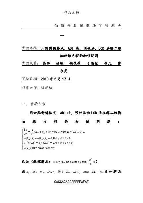
GAGGAGAGGAFFFFAFAF偏微分數值解法實驗報告實驗名稱:六點對稱格式,ADI 法,預校法,LOD 法解二維拋物線方程的初值問題實驗成員: 吳興 楊敏 姚榮華 于瀟龍 余凡 鄭永亮實驗日期:2013年5月17日 指導老師:張建松一、 實驗內容用六點對稱格式,ADI 法,預校法和LOD 法求解二維拋物線方程的初值問題:21(),(,)(0,1)(0,1),0,4(0,,)(1,,)0,01,0,(,0,)(,1,)0,01,0(,,0)sin cos .xx yy y y u u u x y G t t u y t u y t y t u x t u x t x t u x y x y ππ∂⎧=+∈=⨯>⎪∂⎪⎪==<<>⎨⎪==<<>⎪=⎪⎩已知(精確解為:2(,,)sin cos exp()8u x y t x y t πππ=-)設(0,1,,),(0,1,,),(0,1,,)j k n x jh j J y kh k K t n n N τ======差分解為GAGGAGAGGAFFFFAFAF,nj k u ,則邊值條件為:0,,,0,1,1,0,0,1,,,,0,1,,n n k J k nn n nj j j K j K u u k K u u u u j J-⎧===⎪⎨===⎪⎩初值條件為:0,sin cos j k j k u x y ππ=取空間步長12140h h h ===,時間步長11600τ=網比。
1: ADI 法:由第n 层到第n+1层计算分成两步:先先第n 層到n+1/2層,對uxx 用向后差分逼近,對uyy 用向前差分逼近,對uyy 用向后差分逼近,于是得到了如下格式:11112222,,1,,1,,1,,1221222,,2-22=21()n n n n n n n nj kj kj kj k j kj k j k j k n nx j k y j k hh hτδδ+++++-+-+-+-+=+uu uuuu u u (+) (1)u u1111111222,,1,,1,,1,,12212212,,2-22=21()n n n n n n n n j kj kj kj k j kj k j k j k n n x j k y j k hh hτδδ++++++++-+-++-+-+=+u u uuuu u u (+) (2)u u其中j,k=1,2,…,M-1,n=0,1,2,…,上标n+1/2表示在t=tn+1/2+(n+1/2)τ取值。
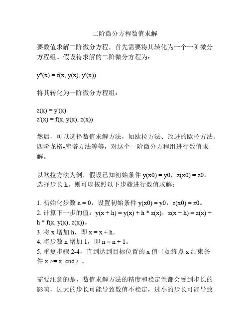
二阶微分方程数值求解
要数值求解二阶微分方程,首先需要将其转化为一个一阶微分方程组。
假设待求解的二阶微分方程为:
y''(x) = f(x, y(x), y'(x))
将其转化为一阶微分方程组:
z(x) = y'(x)
z'(x) = f(x, y(x), z(x))
然后,可以选择数值求解方法,如欧拉方法、改进的欧拉方法、四阶龙格-库塔方法等等,对这个一阶微分方程组进行数值求解。
以欧拉方法为例,假设已知初始条件 y(x0) = y0,z(x0) = z0,
选择步长 h。
则可以按照以下步骤进行数值求解:
1. 初始化步数 n = 0,设置初始条件 y(x0) = y0,z(x0) = z0。
2. 计算下一步的值:y(x + h) = y(x) + h * z(x),z(x + h) = z(x) +
h * f(x, y(x), z(x))。
3. 将 x 增加 h,即 x = x + h。
4. 将步数 n 增加 1,即 n = n + 1。
5. 重复步骤 2-4,直到达到目标位置的 x 值(如终点 x 结束条
件 x >= x_end)。
需要注意的是,数值求解方法的精度和稳定性都会受到步长的影响,过大的步长可能导致数值不稳定,过小的步长可能导致
计算量过大。
因此,选择合适的步长是很重要的。
值得一提的是,当二阶微分方程为边值问题时,可以采用有限差分法、有限元法等数值方法进行数值求解。
这些方法会更为复杂,并涉及到边界条件的处理。
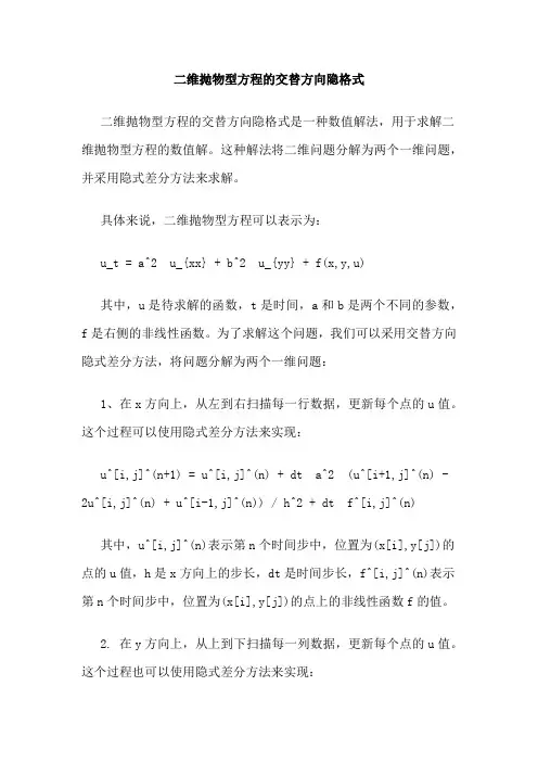
二维抛物型方程的交替方向隐格式二维抛物型方程的交替方向隐格式是一种数值解法,用于求解二维抛物型方程的数值解。
这种解法将二维问题分解为两个一维问题,并采用隐式差分方法来求解。
具体来说,二维抛物型方程可以表示为:u_t = a^2 u_{xx} + b^2 u_{yy} + f(x,y,u)其中,u是待求解的函数,t是时间,a和b是两个不同的参数,f是右侧的非线性函数。
为了求解这个问题,我们可以采用交替方向隐式差分方法,将问题分解为两个一维问题:1、在x方向上,从左到右扫描每一行数据,更新每个点的u值。
这个过程可以使用隐式差分方法来实现:u^[i,j]^(n+1) = u^[i,j]^(n) + dt a^2 (u^[i+1,j]^(n) - 2u^[i,j]^(n) + u^[i-1,j]^(n)) / h^2 + dt f^[i,j]^(n) 其中,u^[i,j]^(n)表示第n个时间步中,位置为(x[i],y[j])的点的u值,h是x方向上的步长,dt是时间步长,f^[i,j]^(n)表示第n个时间步中,位置为(x[i],y[j])的点上的非线性函数f的值。
2. 在y方向上,从上到下扫描每一列数据,更新每个点的u值。
这个过程也可以使用隐式差分方法来实现:u^[i,j]^(n+1) = u^[i,j]^(n) + dt b^2 (u^[i,j+1]^(n) - 2u^[i,j]^(n) + u^[i,j-1]^(n)) / h^2 + dt f^[i,j]^(n) 其中,u^[i,j]^(n)表示第n个时间步中,位置为(x[i],y[j])的点的u值,h是y方向上的步长,dt是时间步长,f^[i,j]^(n)表示第n个时间步中,位置为(x[i],y[j])的点上的非线性函数f的值。
通过交替更新每个点的u值,我们可以逐步逼近方程的数值解。
这种解法具有二阶精度和稳定性,可以应用于多种二维抛物型方程的问题。
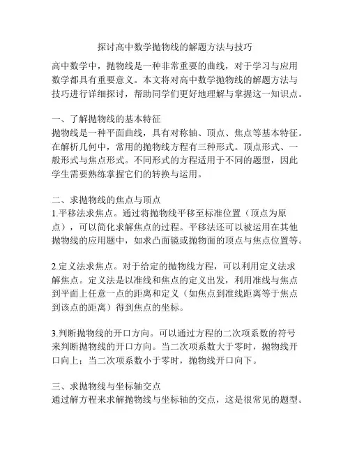
探讨高中数学抛物线的解题方法与技巧高中数学中,抛物线是一种非常重要的曲线,对于学习与应用数学都具有重要意义。
本文将对高中数学抛物线的解题方法与技巧进行详细探讨,帮助同学们更好地理解与掌握这一知识点。
一、了解抛物线的基本特征抛物线是一种平面曲线,具有对称轴、顶点、焦点等基本特征。
在解析几何中,常用的抛物线方程有三种形式。
顶点形式、一般形式与焦点形式。
不同形式的方程适用于不同的题型,因此学生需要熟练掌握它们的转换与运用。
二、求抛物线的焦点与顶点1.平移法求焦点。
通过将抛物线平移至标准位置(顶点为原点),可以简化求解焦点的过程。
平移法还可以被运用在其他抛物线的应用题中,如求凸面镜或抛物面的顶点与焦点位置等。
2.定义法求焦点。
对于给定的抛物线方程,可以利用定义法求解焦点。
定义法是以准线和焦点的定义出发,利用准线与焦点到平面上任意一点的距离和定义(如焦点到准线距离等于焦点到该点的距离)得到焦点的坐标。
3.判断抛物线的开口方向。
可以通过方程的二次项系数的符号来判断抛物线的开口方向。
当二次项系数大于零时,抛物线开口向上;当二次项系数小于零时,抛物线开口向下。
三、求抛物线与坐标轴交点通过解方程来求解抛物线与坐标轴的交点,这是很常见的题型。
有两种常用的方法。
1.因式分解法。
将抛物线的方程进行因式分解后,可以得到解析解或根的个数。
进一步,通过观察与分析,可以得出与坐标轴交点的具体坐标。
2.二次函数求根公式。
通过应用二次函数求根公式,可以得到抛物线与坐标轴交点的解析解。
需要注意的是,二次函数求根公式只适用于已经化为标准形式的抛物线。
四、求抛物线的切线与法线求抛物线的切线与法线是一类较难的题型,需要熟练掌握相关的知识与求解方法。
下面将介绍两种常见的方法。
1.切线与法线的斜率法。
通过斜率法可以求得切线与法线的斜率表达式。
具体而言,对于给定的抛物线方程,我们可以通过计算其导数来求得切线或法线的斜率表达式,然后利用该斜率表达式求解切线或法线的方程。
二维抛物方程的有限差分法二维抛物方程的有限差分法摘要二维抛物方程是一类有广泛应用的偏微分方程,由于大部分抛物方程都难以求得解析解,故考虑采用数值方法求解。
有限差分法是最简单又极为重要的解微分方程的数值方法。
本文介绍了二维抛物方程的有限差分法。
首先,简单介绍了抛物方程的应用背景,解抛物方程的常见数值方法,有限差分法的产生背景和发展应用。
讨论了抛物方程的有限差分法建立的基础,并介绍了有限差分方法的收敛性和稳定性。
其次,介绍了几种常用的差分格式,有古典显式格式、古典隐式格式、Crank-Nicolson隐式格式、Douglas差分格式、加权六点隐式格式、交替方向隐式格式等,重点介绍了古典显式格式和交替方向隐式格式。
进行了格式的推导,分析了格式的收敛性、稳定性。
并以热传导方程为数值算例,运用差分方法求解。
通过数值算例,得出古典显式格式计算起来较简单,但稳定性条件较苛刻;而交替方向隐式格式无条件稳定。
关键词:二维抛物方程;有限差分法;古典显式格式;交替方向隐式格式FINITE DIFFERENCE METHOD FORTWO-DIMENSIONAL PARABOLICEQUATIONAbstractTwo-dimensional parabolic equation is a widely used class of partial differential equations. Because this kind of equation is so complex, we consider numerical methods instead of obtaining analytical solutions. finite difference method is the most simple and extremely important numerical methods for differential equations. The paper introduces the finite difference method for two-dimensional parabolic equation.Firstly, this paper introduces the background and common numerical methods for Parabolic Equation, Background and development of applications. Discusses the basement for the establishment of the finite difference method for parabolic equation And describes the convergence and stability for finite difference method.Secondly, Introduces some of the more common simple differential format,for example, the classical explicit scheme, the classical implicit scheme, Crank-Nicolson implicit scheme, Douglas difference scheme, weighted six implicit scheme and the alternating direction implicit format. The paper focuses on the classical explicit scheme and the alternating direction implicit format. The paper takes discusses the derivation convergence,and stability of the format . The paper takes And the heat conduction equation for the numerical example, using the differential method to solve. Through numerical examples, the classical explicit scheme is relatively simple for calculation, with more stringent stability conditions; and alternating direction implicit scheme is unconditionally stable.Keywords:Two-dimensional Parabolic Equation; Finite-Difference Method; Eclassical Explicit Scheme; Alternating Direction Implicit Scheme1绪论1.1课题背景抛物方程是一类特殊的偏微分方程,二维抛物方程的一般形式为u Lu t ∂=∂ (1-1)其中1212((,,))((,,))(,,)(,,)(,,)u u u u u u L a x y t a x y t b x y t b x y t C x y t x x y y x y∂∂∂∂∂∂=++++∂∂∂∂∂∂ 120,0,0a a C >>≥。
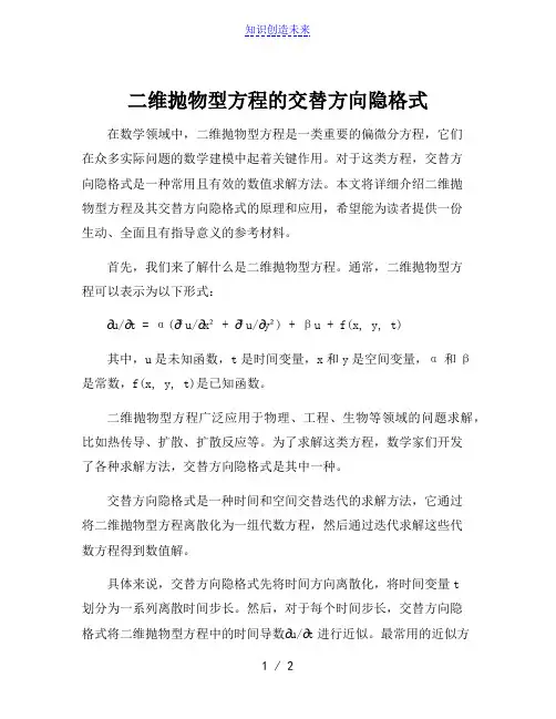
二维抛物型方程的交替方向隐格式在数学领域中,二维抛物型方程是一类重要的偏微分方程,它们在众多实际问题的数学建模中起着关键作用。
对于这类方程,交替方向隐格式是一种常用且有效的数值求解方法。
本文将详细介绍二维抛物型方程及其交替方向隐格式的原理和应用,希望能为读者提供一份生动、全面且有指导意义的参考材料。
首先,我们来了解什么是二维抛物型方程。
通常,二维抛物型方程可以表示为以下形式:∂u/∂t = α(∂²u/∂x² + ∂²u/∂y²) + βu + f(x, y, t)其中,u是未知函数,t是时间变量,x和y是空间变量,α和β是常数,f(x, y, t)是已知函数。
二维抛物型方程广泛应用于物理、工程、生物等领域的问题求解,比如热传导、扩散、扩散反应等。
为了求解这类方程,数学家们开发了各种求解方法,交替方向隐格式是其中一种。
交替方向隐格式是一种时间和空间交替迭代的求解方法,它通过将二维抛物型方程离散化为一组代数方程,然后通过迭代求解这些代数方程得到数值解。
具体来说,交替方向隐格式先将时间方向离散化,将时间变量t划分为一系列离散时间步长。
然后,对于每个时间步长,交替方向隐格式将二维抛物型方程中的时间导数∂u/∂t进行近似。
最常用的近似方法是向后差分格式,即用u(n+1) - u(n)来近似∂u/∂t,其中u(n)表示第n个时间步长的数值解,u(n+1)表示第n+1个时间步长的数值解。
这样,二维抛物型方程可以离散为一组代数方程。
接下来,交替方向隐格式将空间方向离散化,将空间变量x和y划分为一系列离散网格点。
然后,在空间离散化的基础上,通过引入交替方向(例如,先按x方向更新,再按y方向更新,或者反之)和隐格式(例如,使用向后差分格式近似二阶导数项),将二维抛物型方程中的空间导数进行近似。
通过交替迭代求解这组离散代数方程,我们可以得到二维抛物型方程的数值解。
当离散网格点的数量足够多时,数值解将趋近于方程的解。
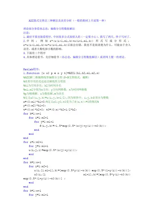
ADI隐式交替法三种解法及误差分析(一般的教材上只说第一种)理论部分参看孙志忠:偏微分方程数值解法注意:1.最好不要直接看程序,中间很多公式很烦人的(一定要小心),我写了两天,终于写对了。
2.中间:例如r*(u(i-1,m1,k)+u(i+1,m1,k))形式写成分形式:r*u(i-1,m1,k)+r*u(i+1,m1,k)后面会出错,我也不是很清楚为什么,可能由于舍入误差,或者大数吃掉小数的影响。
3.下面有三个程序4.具体理论看书,先仔细看书(孙志忠:偏微分方程数值解法)或者网上搜一些理论。
Matlab程序:1.function [u u0 p e x y t]=ADI1(h1,h2,m1,m2,n)%ADI解二维抛物线型偏微分方程(P-R交替隐式,截断)%此程序用的是追赶法解线性方程组%h1为空间步长,h2为时间步长%m1,m2分别为x方向,y方向网格数,n为时间网格数%p为精确解,u为数值解,e为误差%定义u0(i,j,k)=u(i,j,k+1/2),因为矩阵中,i,j,k必须全为整数x=(0:m1)*h1+0;%定义x0,y0,t0是为了f(x,t)~=0的情况%y=(0:m2)*h1+0;t=(0:n)*h2+0; t0=(0:n)*h2+1/2*h2;for k=1:n+1for i=1:m2+1for j=1:m1+1f(i,j,k)=-1.5*exp(0.5*(x(j)+y(i))-t0(k));endendendfor i=1:m2+1for j=1:m1+1u(i,j,1)=exp(0.5*(x(j)+y(i)));endendfor k=1:n+1for i=1:m2+1u(i,[1 m1+1],k)=[exp(0.5*y(i)-t(k)) exp(0.5*(1+y(i))-t(k))]; u0(i,[1 m1+1],k)=[exp(0.5*y(i)-t0(k)) exp(0.5*(1+y(i))-t0(k))] ;endendfor k=1:n+1for j=1:m1+1u([1 m2+1],j,k)=[exp(0.5*x(j)-t(k)) exp(0.5*(1+x(j))-t(k))]; u0([1 m2+1],j,k)=[exp(0.5*x(j)-t0(k)) exp(0.5*(1+x(j))-t0(k))];endendr=h2/(h1*h1);r1=2*(1-r);r2=2*(1+r);for k=1:n %外循环,先固定每一时间层,每一时间层上解一线性方程组% for i=2:m2a=-r*ones(1,m1-1);c=a;a(1)=0;c(m1-1)=0;b=r2*ones(1,m1-1);d(1)=r*u0(i,1,k)+r*(u(i-1,2,k)+u(i+1,2,k))+r1*u(i,2,k)+...h2*f(i,2,k);for l=2:m1-2d(l)=r*(u(i-1,l+1,k)+u(i+1,l+1,k))+r1*u(i,l+1,k)+...h2*f(i,l+1,k);%输入部分系数矩阵,为0的矩阵元素不输入%一定要注意输入元素的正确性endd(m1-1)=r*u0(i,m1+1,k)+r*(u(i-1,m1,k)+u(i+1,m1,k))...+r1*u(i,m1,k)+h2*f(i,m1,k);for l=1:m1-2 %开始解线性方程组消元过程a(l+1)=-a(l+1)/b(l);b(l+1)=b(l+1)+a(l+1)*c(l);d(l+1)=d(l+1)+a(l+1)*d(l);endu0(i,m1,k)=d(m1-1)/b(m1-1); %回代过程%for l=m1-2:-1:1u0(i,l+1,k)=(d(l)-c(l)*u0(i,l+2,k))/b(l);endendfor j=2:m1a=-r*ones(1,m2-1);c=a;a(1)=0;c(m2-1)=0;b=r2*ones(1,m2-1);d(1)=r*u(1,j,k+1)+r*(u0(2,j-1,k)+u0(2,j+1,k))+r1*u0(2,j,k)+...h2*f(2,j,k);for l=2:m2-2d(l)=r*(u0(l+1,j-1,k)+u0(l+1,j+1,k))+r1*u0(l+1,j,k)+... h2*f(l+1,j,k);%输入部分系数矩阵,为0的矩阵元素不输入%一定要注意输入元素的正确性endd(m2-1)=r*u(m2+1,j,k+1)+r*(u0(m2,j-1,k)+u0(m2,j+1,k))...+r1*u0(m2,j,k)+h2*f(m2,j,k);for l=1:m2-2 %开始解线性方程组消元过程a(l+1)=-a(l+1)/b(l);b(l+1)=b(l+1)+a(l+1)*c(l);d(l+1)=d(l+1)+a(l+1)*d(l);endu(m2,j,k+1)=d(m2-1)/b(m2-1); %回代过程%for l=m2-2:-1:1u(l+1,j,k+1)=(d(l)-c(l)*u(l+2,j,k+1))/b(l);endendendfor k=1:n+1for i=1:m2+1for j=1:m1+1p(i,j,k)=exp(0.5*(x(j)+y(i))-t(k)); %p为精确解e(i,j,k)=abs(u(i,j,k)-p(i,j,k)); %e为误差endendend2.function [u p e x y t]=ADI2(h1,h2,m1,m2,n)%ADI解二维抛物线型偏微分方程(D'Yakonov交替方向隐格式)%此程序用的是追赶法解线性方程组%h1为空间步长,h2为时间步长%m1,m2分别为x方向,y方向网格数,n为时间网格数%p为精确解,u为数值解,e为误差%定义u0(i,j,k)=u'(i,j,k)(引入的过渡层),因为矩阵中,i,j,k必须全为整数x=(0:m1)*h1+0;y=(0:m2)*h1+0;t=(0:n)*h2+0;t0=(0:n)*h2+1/2*h2;%定义t0是为了f(x,y,t)~=0的情况% for k=1:n+1for i=1:m2+1for j=1:m1+1f(i,j,k)=-1.5*exp(0.5*(x(j)+y(i))-t0(k));%编程时-t0(k)写成了+t0(k),导致错误;endendend%初始条件for i=1:m2+1for j=1:m1+1u(i,j,1)=exp(0.5*(x(j)+y(i)));endend%边界条件for k=1:n+1for i=1:m2+1u(i,[1 m1+1],k)=[exp(0.5*y(i)-t(k)) exp(0.5*(1+y(i))-t(k))];endendr=h2/(h1*h1);r4=1+r;r5=r/2;for k=1:nfor i=2:m2u0(i,[1 m1+1],k)=r4*u(i,[1 m1+1],k+1)-r5*(u(i-1,[1 m1+1],... k+1)+u(i+1,[1 m1+1],k+1));endendfor k=1:n+1for j=1:m1+1u([1 m2+1],j,k)=[exp(0.5*x(j)-t(k)) exp(0.5*(1+x(j))-t(k))];endendr1=r-r*r;r2=2*(r-1)*(r-1);r3=r*r/2;for k=1:n %外循环,先固定每一时间层,每一时间层上解一线性方程组% for i=2:m2a=-r*ones(1,m1-1);c=a;a(1)=0;c(m1-1)=0;b=2*r4*ones(1,m1-1);d(1)=r*u0(i,1,k)+r1*(u(i-1,2,k)+u(i,1,k)+u(i+1,2,k)+...u(i,3,k))+r2*u(i,2,k)+r3*(u(i-1,1,k)+...u(i+1,1,k)+u(i-1,3,k)+u(i+1,3,k))+2*h2*f(i,2,k);for l=2:m1-2d(l)=r1*(u(i-1,l+1,k)+u(i,l,k)+u(i+1,l+1,k)+...u(i,l+2,k))+r2*u(i,l+1,k)+r3*(u(i-1,l,k)+...u(i+1,l,k)+u(i-1,l+2,k)+u(i+1,l+2,k))+2*h2*f(i,l+1,k);%输入部分系数矩阵,为0的矩阵元素不输入%一定要注意输入元素的正确性endd(m1-1)=r*u0(i,m1+1,k)+r1*(u(i-1,m1,k)+u(i,m1-1,k)+...u(i+1,m1,k)+u(i,m1+1,k))+r2*u(i,m1,k)+...r3*(u(i-1,m1-1,k)+...u(i+1,m1-1,k)+u(i-1,m1+1,k)+u(i+1,m1+1,k))+2*h2*f(i,m1,k);for l=1:m1-2 %开始解线性方程组消元过程a(l+1)=-a(l+1)/b(l);b(l+1)=b(l+1)+a(l+1)*c(l);d(l+1)=d(l+1)+a(l+1)*d(l);end%回代过程%u0(i,m1,k)=d(m1-1)/b(m1-1);for l=m1-2:-1:1u0(i,l+1,k)=(d(l)-c(l)*u0(i,l+2,k))/b(l);endendfor j=2:m1a=-r*ones(1,m2-1);c=a;a(1)=0;c(m2-1)=0;b=2*r4*ones(1,m2-1);d(1)=r*u(1,j,k+1)+2*u0(2,j,k);for l=2:m2-2d(l)=2*u0(l+1,j,k);%输入部分系数矩阵,为0的矩阵元素不输入%一定要注意输入元素的正确性endd(m2-1)=2*u0(m2,j,k)+r*u(m2+1,j,k+1);for l=1:m2-2 %开始解线性方程组消元过程a(l+1)=-a(l+1)/b(l);b(l+1)=b(l+1)+a(l+1)*c(l);d(l+1)=d(l+1)+a(l+1)*d(l);endu(m2,j,k+1)=d(m2-1)/b(m2-1); %回代过程%for l=m2-2:-1:1u(l+1,j,k+1)=(d(l)-c(l)*u(l+2,j,k+1))/b(l);endendendfor k=1:n+1for i=1:m2+1for j=1:m1+1p(i,j,k)=exp(0.5*(x(j)+y(i))-t(k)); %p为精确解e(i,j,k)=abs(u(i,j,k)-p(i,j,k)); %e为误差endendend3.function [u u0 p e x y t]=ADI5(h1,h2,m1,m2,n)%ADI解二维抛物线型偏微分方程(P-R交替隐式,未截断)%此程序用的是追赶法解线性方程组%h1为空间步长,h2为时间步长%m1,m2分别为x方向,y方向网格数,n为时间网格数%p为精确解,u为数值解,e为误差%定义u0(i,j,k)=u(i,j,k+1/2),因为矩阵中,i,j,k必须全为整数x=(0:m1)*h1+0;%定义x0,y0,t0是为了f(x,t)~=0的情况%y=(0:m2)*h1+0;t=(0:n)*h2+0; t0=(0:n)*h2+1/2*h2;for k=1:n+1for i=1:m2+1for j=1:m1+1f(i,j,k)=-1.5*exp(0.5*(x(j)+y(i))-t0(k));endendendfor i=1:m2+1for j=1:m1+1u(i,j,1)=exp(0.5*(x(j)+y(i)));endendfor k=1:n+1for i=1:m2+1u(i,[1 m1+1],k)=[exp(0.5*y(i)-t(k)) exp(0.5*(1+y(i))-t(k))]; u1(i,[1 m1+1],k)=[exp(0.5*y(i)-t0(k)) exp(0.5*(1+y(i))-t0(k))] ;endendr=h2/(h1*h1);r1=2*(1-r);r2=r/4;r3=2*(1+r);for k=1:nfor i=2:m2u0(i,[1 m1+1],k)=u1(i,[1 m1+1],k)-r2*(u(i-1,[1 m1+1],k+1)-...2*u(i,[1 m1+1],k+1)+u(i+1,[1 m1+1],k+1)-u(i-1,[1 m1+1],k)+...2*u(i,[1 m1+1],k)-u(i+1,[1 m1+1],k));endendfor k=1:n+1for j=1:m1+1u([1 m2+1],j,k)=[exp(0.5*x(j)-t(k)) exp(0.5*(1+x(j))-t(k))];endendfor k=1:n %外循环,先固定每一时间层,每一时间层上解一线性方程组%for i=2:m2a=-r*ones(1,m1-1);c=a;a(1)=0;c(m1-1)=0;b=r3*ones(1,m1-1);d(1)=r*u0(i,1,k)+r*(u(i-1,2,k)+u(i+1,2,k))+r1*u(i,2,k)+... h2*f(i,2,k);for l=2:m1-2d(l)=r*(u(i-1,l+1,k)+u(i+1,l+1,k))+r1*u(i,l+1,k)+...h2*f(i,l+1,k);%输入部分系数矩阵,为0的矩阵元素不输入%一定要注意输入元素的正确性endd(m1-1)=r*u0(i,m1+1,k)+r*(u(i-1,m1,k)+u(i+1,m1,k))...+r1*u(i,m1,k)+h2*f(i,m1,k);for l=1:m1-2 %开始解线性方程组消元过程a(l+1)=-a(l+1)/b(l);b(l+1)=b(l+1)+a(l+1)*c(l);d(l+1)=d(l+1)+a(l+1)*d(l);endu0(i,m1,k)=d(m1-1)/b(m1-1); %回代过程%for l=m1-2:-1:1u0(i,l+1,k)=(d(l)-c(l)*u0(i,l+2,k))/b(l);endendfor j=2:m1a=-r*ones(1,m2-1);c=a;a(1)=0;c(m2-1)=0;b=r3*ones(1,m2-1);d(1)=r*u(1,j,k+1)+r*(u0(2,j-1,k)+u0(2,j+1,k))+r1*u0(2,j,k)+...h2*f(2,j,k);for l=2:m2-2d(l)=r*(u0(l+1,j-1,k)+u0(l+1,j+1,k))+r1*u0(l+1,j,k)+... h2*f(l+1,j,k);%输入部分系数矩阵,为0的矩阵元素不输入%一定要注意输入元素的正确性endd(m2-1)=r*u(m2+1,j,k+1)+r*(u0(m2,j-1,k)+u0(m2,j+1,k))...+r1*u0(m2,j,k)+h2*f(m2,j,k);for l=1:m2-2 %开始解线性方程组消元过程a(l+1)=-a(l+1)/b(l);b(l+1)=b(l+1)+a(l+1)*c(l);d(l+1)=d(l+1)+a(l+1)*d(l);endu(m2,j,k+1)=d(m2-1)/b(m2-1); %回代过程%for l=m2-2:-1:1u(l+1,j,k+1)=(d(l)-c(l)*u(l+2,j,k+1))/b(l);endendendfor k=1:n+1for i=1:m2+1for j=1:m1+1p(i,j,k)=exp(0.5*(x(j)+y(i))-t(k)); %p为精确解 e(i,j,k)=abs(u(i,j,k)-p(i,j,k)); %e为误差endendend[up e x y t]=ADI2(0.01,0.001,100,100,1000);surf(x,y,e(:,:,1001)) t=1的误差曲面下面是三种方法的误差比较:1.[u u0 p e x y t]=ADI1(0.1,0.1,10,10,10)((P-R交替隐式,截断)截断中间过渡层用u(i,j,k+1/2)代替)(t=1时的误差)2.[u u0 p e x y t]=ADI5(0.1,0.1,10,10,10)(P-R交替隐式,未截断)(未截断过渡层u(i,j,)’=u(i,j,k+1/2)-h2^2/4*dy^2dtu(i,j,k+1/2);)3.[u p e x y t]=ADI2(0.1,0.1,10,10,10)(D'Yakonov交替方向隐格式) surf(x,y,e(:,:,11))(表示t=1时的误差)下面是相关数据:1: [u u0 p e x y t]=ADI1(0.1,0.1,10,10,10)((P-R交替隐式,截断)截断中间过渡层用u(i,j,k+1/2)代替)e(:,:,11) =Columns 1 through 60 0 0 0 0 00 0.00040947 0.00025182 0.00019077 0.00017112 0.000176040 0.00057359 0.00042971 0.00035402 0.00032565 0.000336280 0.00066236 0.00054689 0.00047408 0.00044596 0.000462670 0.00072152 0.00062001 0.00055081 0.00052442 0.000545530 0.00076164 0.0006576 0.00058522 0.00055732 0.000579840 0.00078336 0.00065993 0.00057557 0.00054161 0.000562090 0.00078161 0.00061872 0.00051646 0.00047429 0.000489640 0.00073621 0.0005148 0.00039979 0.00035439 0.000363130 0.00056964 0.00031688 0.00022051 0.0001884 0.000191920 0 0 0 0 02.[u u0 p e x y t]=ADI5(0.1,0.1,10,10,10)(P-R交替隐式,未截断)(未截断过渡层u(i,j,)’=u(i,j,k+1/2)-h2^2/4*dy^2dtu(i,j,k+1/2);)e(:,:,11) =Columns 1 through 60 0 0 0 0 00 0.00027006 0.00016305 0.00012104 0.0001071 0.000109950 0.00037754 0.00027817 0.0002253 0.00020483 0.000211160 0.00043539 0.00035386 0.00030207 0.00028124 0.00029140 0.00047398 0.00040104 0.00035113 0.00033111 0.000344050 0.0005003 0.00042535 0.00037309 0.0003519 0.000365710 0.00051479 0.00042699 0.00036681 0.00034164 0.00035410 0.00051415 0.00040056 0.00032887 0.0002985 0.000307640 0.00048504 0.0003335 0.00025411 0.0002221 0.000227060 0.00037609 0.00020532 0.00013956 0.00011718 0.000119020 0 0 0 0 03.[u p e x y t]=ADI2(0.1,0.1,10,10,10)(D'Yakonov交替方向隐格式)e(:,:,11) =Columns 1 through 60 0 0 0 0 00 8.6469e-006 1.4412e-005 1.8364e-005 2.091e-005 2.2174e-0050 1.4412e-005 2.4777e-005 3.2047e-005 3.6716e-005 3.8961e-0050 1.8364e-005 3.2047e-005 4.1789e-005 4.8054e-005 5.1008e-0050 2.091e-005 3.6716e-005 4.8054e-005 5.5353e-005 5.8764e-0050 2.2174e-005 3.8961e-005 5.1008e-005 5.8764e-005 6.2389e-0050 2.2118e-005 3.8698e-005 5.0523e-005 5.8126e-005 6.171e-0050 2.055e-005 3.5581e-005 4.6157e-005 5.2942e-005 5.6197e-0050 1.707e-005 2.8951e-005 3.7128e-005 4.2365e-005 4.4952e-0050 1.0851e-005 1.7698e-005 2.2265e-005 2.5203e-005 2.672e-0050 0 0 0 0 01.[u u0 p e x y t]=ADI1(0.1,0.1,10,10,10)((P-R交替隐式,截断)截断中间过渡层用u(i,j,k+1/2)代替)Columns 7 through 110 0 0 0 00.00020348 0.00026228 0.00038338 0.00066008 00.00038607 0.00048321 0.00064717 0.00091668 00.00052635 0.00064203 0.00081637 0.0010517 00.0006174 0.00074272 0.00092111 0.0011417 00.00065651 0.00078964 0.00097724 0.0012051 00.00064051 0.00078116 0.00098594 0.0012433 00.00056474 0.00070822 0.00093332 0.0012478 00.00042547 0.00055526 0.00078616 0.0011844 00.00022735 0.00030946 0.00049004 0.00092402 00 0 0 0 02.[u u0 p e x y t]=ADI5(0.1,0.1,10,10,10)(P-R交替隐式,未截断)(未截断过渡层u(i,j,)’=u(i,j,k+1/2)-h2^2/4*dy^2dtu(i,j,k+1/2);)Columns 7 through 110 0 0 0 00.00012826 0.00016798 0.00024986 0.00043637 00.00024444 0.00031023 0.00042173 0.00060513 00.00033401 0.00041257 0.00053179 0.00069358 00.00039216 0.00047742 0.00059986 0.00075263 00.00041704 0.00050761 0.00063642 0.00079439 00.00040657 0.0005021 0.00064226 0.00081984 00.00035784 0.000455 0.00060828 0.00082334 00.00026866 0.00035628 0.00051263 0.0007824 00.00014262 0.00019789 0.00031956 0.0006113 00 0 0 0 0 3.[u p e x y t]=ADI2(0.1,0.1,10,10,10)(D'Yakonov交替方向隐格式) Columns 7 through 110 0 0 0 02.2118e-005 2.055e-005 1.707e-005 1.0851e-005 03.8698e-005 3.5581e-005 2.8951e-005 1.7698e-005 05.0523e-005 4.6157e-005 3.7128e-005 2.2265e-005 05.8126e-005 5.2942e-005 4.2365e-005 2.5203e-005 06.171e-005 5.6197e-005 4.4952e-005 2.672e-005 06.1116e-005 5.5803e-005 4.4817e-005 2.6785e-005 05.5803e-005 5.1239e-005 4.1529e-005 2.5153e-005 04.4817e-005 4.1529e-005 3.42e-005 2.126e-005 02.6785e-005 2.5153e-005 2.126e-005 1.3869e-005 00 0 0 0 0。
抛物线方程解法抛物线是一种常见的曲线形式,它在物理学、工程学和数学中都有广泛的应用。
抛物线方程是描述抛物线形状的数学表达式,通常采用二次方程的形式。
在本文中,我们将介绍如何通过抛物线方程来解决相关问题。
抛物线方程的一般形式为 y = ax^2 + bx + c,其中 a、b、c 是常数,x 和 y 分别表示坐标轴上的点的横坐标和纵坐标。
我们可以通过已知的条件,如焦点、顶点和对称轴等,来确定抛物线方程的具体形式。
让我们来看一个简单的例子,以帮助理解抛物线方程的解法。
假设我们已知一个抛物线的焦点为 (1,2),并且过顶点 (0,0)。
我们的目标是找到抛物线的方程。
根据抛物线的定义,我们知道焦点到顶点的距离等于焦点到抛物线上任意一点的距离。
因此,我们可以使用焦点和顶点的信息来确定常数 a 的值。
在这个例子中,焦点到顶点的距离是 2,因此 a = 1/2a。
由此得到抛物线方程的一部分: y = 1/2ax^2 + bx + c。
接下来,我们可以使用顶点的信息来确定常数 b 和 c 的值。
由于顶点 (0,0) 在抛物线上,我们可以将其代入抛物线方程中,得到 c = 0。
此时,抛物线方程变为 y = 1/2ax^2 + bx。
现在,我们还需要确定常数 b 的值。
由于我们已知焦点 (1,2) 在抛物线上,我们可以将其代入抛物线方程中,得到 2 = 1/2a + b。
根据这个方程,我们可以求解出常数 b 的值。
通过以上步骤,我们成功地找到了抛物线方程的解法。
最终的抛物线方程为 y = 1/2x^2 + 3/2x。
除了上述例子中的解法,我们还可以通过其他已知条件来确定抛物线方程。
例如,如果我们已知抛物线的对称轴是 x = 1,我们可以利用这个信息来推导出抛物线方程。
对称轴是抛物线的镜像轴,因此对称轴上的点到焦点的距离等于对称轴上的点到抛物线上任意一点的距离。
通过将对称轴上的点 (1,y) 代入抛物线方程,并根据已知条件求解常数 a 和 c 的值,可以得到抛物线方程。
%%%%%%%%%%%%%%%%%%%%%%%%%%%%%%%%%%%%%%%%%% %%%%%%%%%%%%%%%%%%%%%%%%%%%%%% % % % Example of ADI Method for 2D heat equation % % % % u_t = u_{xx} + u_{yy} + f(x,t) % %a<x<b;c<y<d % % Test problme: % % Exact solution: u(t,x,y) = exp(-t) sin(pi*x)sin(pi*y) % % Source term: f(t,x,y) = exp(-t) sin(pi*x) sin(pi*y) (2pi^2-1) % % % % Files needed for the test: % % % % adi.m: This file, the main calling code. % % f.m: The file defines the f(t,x,y) % % uexact.m: The exactsolution. % %%%%%%%%%%%%%%%%%%%%%%%%%%%%%%%%%%%% %%%%%%%%%%%%%%%%%%%%%%%%%%%%%%%%%%%% clear; close all; a = 0; b=1; c=0; d=1; n = 40; tfinal = 1; m = n; h = (b-a)/n; dt=h; h1 = h*h; r=dt/h1; x=a:h:b; y=c:h:d; %-- Initial condition: t = 0; for i=1:m+1, for j=1:m+1, u1(i,j) = uexact(t,x(i),y(j)); end end %---------- Big loop for time t -------------------------------------- k_t = fix(tfinal/dt); for k=1:k_t t1 = t + dt; t2 = t + dt/2; %--- sweep in x-direction -------------------------------------- for i=2:m, % Boundary condition. u2(1,i) = -r/2*uexact(t1,x(1),y(i-1)) + (1+r)*uexact(t1,x(1),y(i)) + -r/2*uexact(t1,x(1),y(i+1));u2(m+1,i) = -r/2*uexact(t1,x(m+1),y(i-1)) + (1+r)*uexact(t1,x(m+1),y(i)) + -r/2*uexact(t1,x(m+1),y(i+1)); end for j = 2:n, % Look for fixed y(j) b=zeros(m-1,1); for i=2:m, b(i-1) = r^2/4*( u1(i-1,j-1) + u1(i-1,j+1) + u1(i+1,j-1) + u1(i+1,j+1) ) ... +r/2*( 1-r )*( u1(i-1,j) + u1(i+1,j) + u1(i,j-1) + u1(i,j+1) )... + ( 1-2*r+r^2 )*u1(i,j) -3/2*dt*exp( 1/2*( (i-1)*h + (j-1)*h ) -t2 ); end b(1) = b(1) + r/2 * u2(1,j); b(m-1) =b(m-1) + r/2 * u2(m+1,j); A = diag( (1+r)*ones(m-1,1) ) + diag( -r/2*ones(m-2,1),1 ) ... + diag(-r/2*ones(m-2,1),-1); ut = A\b; % Solve the diagonal matrix. for i=1:m-1,u2(i+1,j) = ut(i); end end % Finish x-sweep. %-------------- loop in y -direction -------------------------------- for i=1:m+1, % Boundary condition u1(i,1) = uexact(t1,x(i),y(1));u1(i,n+1) = uexact(t1,x(i),y(m+1)); u1(1,i) = uexact(t1,x(1),y(i)); u1(m+1,i) =uexact(t1,x(m+1),y(i)); end for i = 2:m, for j=2:m, b(j-1) = u2(i,j); end b(1) = b(1) + r/2*u1(i,1); b(m-1) = b(m-1) + r/2*u1(i,m+1);A = diag( (1+r)*ones(m-1,1) ) + diag( -r/2*ones(m-2,1),1 ) ... + diag(-r/2*ones(m-2,1),-1); ut = A\b; for j=1:n-1, u1(i,j+1) = ut(j); end end % Finish y-sweep. t = t + dt; %--- finish ADI method at this time level, go to the next time level. end %-- Finished with the loop in time %----------- Data analysis ---------------------------------- for i=1:m+1, for j=1:n+1, ue(i,j) = uexact(tfinal,x(i),y(j)); end end [xx,yy]=meshgrid(x,y); xx=xx';yy=yy'; mesh(xx,yy,u1) title('数值解图') pause surf(xx,yy,ue) title('精确解图') pausesurf(xx,yy,u1-ue) title('误差图') e = max(max(abs(u1-ue))) % The infinityerror. %******%表示原来程序编写错误 %%%%%%%%%%%%%%%%%%%%%%%%%%%%%%%%%%%%%%%% %%%%%%%%%%%%%%%%%%%%%%%%%%%%%%%% % % % Example of ADI Method for 2D heat equation % % % % u_tt = u_{xx} + u_{yy} + f(x,t) % %a<x<b;c<y<d % % Test problme: % % 精确解: u(t,x,y) = exp( 1/2*(x+y) - t ) % % 右端函数: f(t,x,y) = 1/2*exp( 1/2*(x+y) - t ) % % 初始条件: g1 = exp( 1/2*(x+y) ) % % 初始导数条件: g2 = -exp( 1/2*(x+y) ) % % 需要函数 % % g1.m g2.m 初始条件 % % f2.m: The file defines the f(t,x,y) % % uexact.m: The exactsolution. % %%%%%%%%%%%%%%%%%%%%%%%%%%%%%%%%%%%% %%%%%%%%%%%%%%%%%%%%%%%%%%%%%%%%%%%% clear; close all; a = 0; b=1; c=0; d=1; n = 10; tfinal = 1; m = n; h = (b-a)/n; dt=h; s=(dt/h)^2; x=a:h:b; y=c:h:d; %-- Initial condition: t = 0; for i=1:m+1, for j=1:m+1, u1(i,j) = g1(x(i),y(j)); end end %-- Initial deriavtive condition: for i=1:m+1, for j=1:m+1, %******% u2(i,j) = g1(x(i),y(j)) + dt * g2( x(i),y(j) ) + dt^2/4 * ( g1(x(i),y(j)) + f2 (t, x(i),y(j) ) ); u2(i,j) =g1(x(i),y(j)) + dt * g2( x(i),y(j) ) + dt^2/2 * ( g1(x(i),y(j))/2 + f2 (t, x(i),y(j) ) ); endend %---------- Big loop for time t -------------------------------------- k_t = fix(tfinal/dt); for k=2:k_t t1 = t + dt; t2 = t1 + dt; %--- sweep in x-direction --------------------------------------for i=1:m+1, % Boundary condition. u4(1,i) = ( uexact(t,x(1),y(i)) -2*uexact(t1,x(1),y(i)) + uexact(t2,x(1),y(i)) )/dt^2 ; u4(m+1,i) = ( uexact(t,x(m+1),y(i)) - 2*uexact(t1,x(m+1),y(i)) + uexact(t2,x(m+1),y(i)) )/dt^2 ; u4(i,1) = ( uexact(t,x(i),y(1)) - 2*uexact(t1,x(i),y(1)) + uexact(t2,x(i),y(1)) )/dt^2 ; u4(i,m+1) = ( uexact(t,x(i),y(m+1)) - 2*uexact(t1,x(i),y(m+1)) + uexact(t2,x(i),y(m+1)) )/dt^2 ; end for i=2:m u3(1,i)=-s/2*u4(1,i-1) + (1+s)*u4(1,i) - s/2*u4(1,i+1); u3(m+1,i)=-s/2*u4(m+1,i-1) +(1+s)*u4(m+1,i) - s/2*u4(m+1,i+1); end for j = 2:n, % Look for fixed y(j) b=zeros(m-1,1); for i=2:m, b(i-1) = ( u2(i-1,j) + u2(i+1,j) + u2(i,j-1) + u2(i,j+1) -4*u2(i,j) )/h^2 +f2 (t1, x(i),y(j) ); end b(1) = b(1) + s/2 * u3(1,j); b(m-1) = b(m-1) + s/2 * u3(m+1,j); A = diag( (1+s)*ones(m-1,1) ) + diag( -s/2*ones(m-2,1),1 ) ... + diag(-s/2*ones(m-2,1),-1); ut = A\b; % Solve the diagonal matrix. for i=1:m-1, u3(i+1,j) = ut(i); end end % Finish x-sweep. %-------------- loop in y -direction -------------------------------- for i = 2:m, forj=2:m, b(j-1) = u3(i,j); end b(1) = b(1) + s/2*u4(i,1); b(m-1) = b(m-1) + s/2*u4(i,m+1); ut = A\b; for j=1:n-1, u4(i,j+1) = ut(j); end end % Finish y-sweep. for i=1:m+1, % Boundary condition u5(i,1) = uexact(t2,x(i),y(1)); u5(i,m+1) = uexact(t2,x(i),y(m+1));u5(1,i) = uexact(t2,x(1),y(i)); u5(m+1,i) = uexact(t2,x(m+1),y(i)); end for i=2:m, forj=2:m, u5(i,j) = dt^2 * u4(i,j) + 2*u2(i,j) - u1(i,j); end end u1=u2; u2=u5; %******%t = t2 + dt; t = t+dt ; %--- finish ADI method at this time level, go to the next time level. end %-- Finished with the loop in time %----------- Data analysis ---------------------------------- for i=1:m+1, for j=1:n+1, ue(i,j) = uexact(tfinal,x(i),y(j)); end end[xx,yy]=meshgrid(x,y); xx=xx';yy=yy'; mesh(xx,yy,u2) title('数值解图') pausesurf(xx,yy,ue) title('精确解图') pause %******%surf(xx,yy,u2-ue) surf(xx,yy,u2-ue) title('误差图') e = max(max(abs(u2-ue))) %******%e = max(max(abs(u1-ue))) % The infinityerror. %%%%%%%%%%%%%%%%%%%%%%%%%%%%%%%%%%%%%%% %%%%%%%%%%%%%%%%%%%%%%%%%%%%%%%%% % % % Example of ADI Method for 2D heat equation % % % % u_t = u_{xx} + u_{yy} + f(x,t) % %a<x<b;c<y<d % % Test problme: % % Exact solution: u(t,x,y) = exp(-t) sin(pi*x) sin(pi*y) % % Source term: f(t,x,y) = exp(-t) sin(pi*x) sin(pi*y) (2pi^2-1) % % % % Files needed for the test: % % % % f.m: The file defines the f(t,x,y) % % uexact.m: The exact solution. % %%%%%%%%%%%%%%%%%%%%%%%%%%%%%%%%%%%% %%%%%%%%%%%%%%%%%%%%%%%%%%%%%%%%%%%% clear; close all; a = 0; b=1; c=0; d=1; n = 20; tfinal = 1; m = n; h = (b-a)/n; h1 = h*h; dt=h1; r=dt/h1; x=a:h:b; y=c:h:d; %-- Initial condition: t = 0; for i=1:m+1, for j=1:m+1, u1(i,j) = uexact(t,x(i),y(j)); end end %---------- Big loop for time t -------------------------------------- k_t = ceil(tfinal/dt); for k=1:k_t t1 = t + dt; t2 = t + dt/2; %--- sweep in x-direction -------------------------------------- for j=2:m, % Boundary condition. u2(1,j) = (1/12-r/2)*uexact(t1,x(1),y(j-1)) + (5/6+r)*uexact(t1,x(1),y(j)) + (1/12-r/2) *uexact(t1,x(1),y(j+1)); u2(m+1,j) = (1/12-r/2)*uexact(t1,x(m+1),y(j-1)) +(5/6+r)*uexact(t1,x(m+1),y(j)) + (1/12-r/2) * uexact(t1,x(m+1),y(j+1)); end for j =2:n, % Look for fixed y(j) b=zeros(m-1,1); for i=2:m, b(i-1) = (1/144+r/12+r^2/4) * ( u1(i-1,j-1) + u1(i-1,j+1) + u1(i+1,j-1) + u1(i+1,j+1) ) ... + ( 10/144+r/3-r^2/2 )*( u1(i-1,j) + u1(i+1,j) + u1(i,j-1) + u1(i,j+1) )... + ( 100/144 - 40 * r/24 + r^2 )*u1(i,j)... + dt * ( f(t2,x(i-1),y(j-1)) + f(t2,x(i-1),y(j+1)) + f(t2,x(i+1),y(j-1)) + f(t2,x(i+1),y(j+1))... + 10 * ( f(t2,x(i-1),y(j)) + f(t2,x(i+1),y(j)) + f(t2,x(i),y(j-1)) + f(t2,x(i),y(j+1)) )... + 100 *f(t2,x(i),y(j)) ) / 144; end b(1) = b(1) + ( r/2 -1/12 ) * u2(1,j); b(m-1) = b(m-1) + ( r/2 -1/12 ) * u2(m+1,j); A = diag( (5/6+r)*ones(m-1,1) ) + diag( (1/12-r/2) * ones(m-2,1),1 ) ... + diag( (1/12-r/2) * ones(m-2,1),-1); ut = A\b; % Solve the diagonal matrix. for i=1:m-1, u2(i+1,j) = ut(i); end end % Finish x-sweep. %-------------- loop in y -direction -------------------------------- for i=1:m+1, % Boundary condition u1(i,1) = uexact(t1,x(i),y(1)); u1(i,n+1) = uexact(t1,x(i),y(m+1)); u1(1,i) = uexact(t1,x(1),y(i));u1(m+1,i) = uexact(t1,x(m+1),y(i)); end for i = 2:m, for j=2:m, b(j-1) = u2(i,j); end b(1) =b(1) + ( r/2 -1/12 ) * u1(i,1); b(m-1) = b(m-1) + ( r/2 -1/12 ) * u1(i,m+1); ut = A\b; for j=1:n-1, u1(i,j+1) = ut(j); end end % Finish y-sweep. t = t + dt; %--- finish ADI method at this time level, go to the next time level. end %-- Finished with the loop in time %----------- Data analysis ---------------------------------- for i=1:m+1, for j=1:n+1, ue(i,j) = uexact(tfinal,x(i),y(j)); end end [xx,yy]=meshgrid(x,y); xx=xx';yy=yy'; mesh(xx,yy,u1) title('数值解图') pause surf(xx,yy,ue) title('精确解图') pause surf(xx,yy,u1-ue) title('误差图') e = max(max(abs(u1-ue))) % The infinity error. %算例1.1.3,见课本第17页 %首先网格剖分 xl=0.; xr=pi;%左右端点 n=20; h=(xr-xl)/n;%步长 %解差分格式形成的方程组 U=zeros(n-1,1); aa=-1+h^2/12; bb=2+5/6*h^2; A=diag(bb*ones(n-1,1))+diag(aa*ones(n-2,1),1)+diag(aa*ones(n-2,1),-1);%系数矩阵 F=zeros(n-1,1); for i=1:n-1 F(i)=h^2/12*(exp(xl+(i-1)*h)*(sin(xl+(i-1)*h)-2*cos(xl+(i-1)*h))+10*exp(xl+i*h)*(sin(xl+i*h)-2*cos(xl+i*h))+exp(xl+(i+1)*h)*(sin(xl+(i+1)*h)-2*cos(xl+(i+1)*h)));%右端项 end U=inv(A)*F;%得到数值解 %精确解与数值解误差绝对值的最大值 ana=zeros(n-1,1); for i=1:n-1 ana(i)=exp(xl+i*h)*sin(xl+i*h);%精确解 end wucha=max(abs(U-ana)) %可视化处理 x=xl:h:xr; U=[0 U' 0];%U表示数值解ana=[0 ana' 0];%ana表示精确解 plot(x,U,'r*',x,ana); %向后Euler差分格式 %Ut-Uxx=0,0<x<1,0<t<1 %u(x,0)=exp(x) %u(0,t)=exp(t),u(1,t)=exp(1+t) %%%%%%%网格剖分%%%%%%%%% % first set up the attributes h = 0.1; % the step-size in the x dimension%空间步长 r=1; %步长比 dt = h^2 * r; % the step-size in the t dimension%%时间步长 T0 = 1; % the time-interval over which we will calculate u 时间长度 TN = ceil(T0 / dt); % the number of steps in the time-interval%时间网格 X0 = 1; % the x-interval over which we will calculate u空间长度 XN = ceil(X0 / h); % the number of steps in the x-interval%空间网格 U = zeros(XN + 1, TN + 1); % set up an array of zeros %初始化 % Next we set up the initial conditions%初始值及边界值 x = 0 :h: X0; for j=1:XN+1 U(j , 1) = exp( (j-1)*h ); end for k=1:TN+1 U(1,k) =exp( (k-1) *dt);U(XN+1,k)=exp(1+ ( k-1 ) *dt); end %%%%%%形成系数矩阵%%%%%%%% A=diag((5/6+r)*ones(XN-1,1))+diag( (1/12-r/2) *ones(XN-2,1),1 )+diag( (1/12-r/2)*ones(XN-2,1),-1 ); B=diag((5/6-r)*ones(XN-1,1))+diag( (1/12+r/2) *ones(XN-2,1),1 )+diag( (1/12+r/2)*ones(XN-2,1),-1 ); %右端项初始化 F = zeros( XN-1,1 ); %迭代求解 for k = 1 : TN F(1)=(1/12+r/2)*exp((k-1)*dt)-(1/12-r/2)*exp(k*dt); F(XN-1)=(1/12+r/2)*exp((k-1)*dt+1)-(1/12-r/2)*exp(k*dt+1); U(2:XN,k+1)= A \ ( B * U(2:XN,k) + F ); end; %给出精确解 ana = zeros(XN + 1, TN + 1); for k = 1 : TN+1 for j = 1 : XN+1 ana(j, k ) = exp ( (j-1) *h + (k-1)*dt); end; end; %给出在T=1时的最大误差 max( abs ( U (:,TN+1) -ana (:,TN+1) ) ) %图示化 t=0:dt:T0; [xx,tt]= meshgrid(x,t); xx=xx'; tt=tt'; mesh(xx,tt,ana); title('analytical solution');ylabel(sprintf('steps in x domain\nfrom 0 to 1')); xlabel(sprintf('steps in time-domain\nfrom 0 to 1')); zlabel('U(x,y)'); pause mesh(xx,tt,U); title('numerical solution'); ylabel(sprintf('steps in x domain\nfrom 0 to 1')); xlabel(sprintf('steps in time-domain\nfrom 0 to 1')); zlabel('U(xi,tk)'); pause mesh(xx,tt,U-ana); title('diffeence beween analical and numeical soluion'); ylabel(sprintf('steps in x domain\nfrom 0 to 1')); xlabel(sprintf('steps in time-domain\nfrom 0 to 1')); zlabel('U(xi,tk)'); pauseplot(x,U(:,TN+1),'-or',x,ana(:,TN+1)) title('向前Euler格式数值解与精确解的比较') legend('uh(x,1)','u(x,1)')%Crank-Nicolson schemes % 显差分格式 %算例4.1.1 %%%%%%%网格剖分%%%%%%%%% h = 1/10; %%空间步长 a = 1; dt =1/20; %时间步长 s = a * dt/h; %步长比 T = 1; % 时间长度 n = ceil(T / dt); % 时间网格 X0 = 1; % 空间长度 m = ceil(X0 / h); %空间网格 u = zeros(n + 1, m + 1); %%数解初始化u(tk,xi) % %初始值及边界值 x=0:h:X0; phi=exp(x); u(1,:)=phi; %u的第一行表示初始状态 t=0:dt:T; u(:,1)=exp(t'); %左界u(:,m+1)=exp(1+t'); %%%%%%%%%%%%%%% f=zeros(n-1,m-1); for k=1:n+1 for i=1:m+1 f(k,i)=0; end end %%%%%%%%%%%%%%% psi=exp(x); for i = 2:m u(2,i) = dt * psi(i) + s^2/2 * ( phi(i-1) + phi(i+1) ) ... + ( 1 - s^2 ) * phi(i) + dt^2/2 * f(1,i);end %%%%%%%%%%%%%%% for k=2:n for i=2:m u (k+1 , i) = s^2 * u (k , i-1) +2*( 1-s^2 )*u (k , i) ... + s^2 * u (k , i+1) - u (k-1 , i) + dt^2 * f( k , i); endend %%%%%%%%%%%%%%%%给出精确解 ana = zeros(n + 1, m + 1); for k = 1 : n+1 for i = 1 : m+1 ana( k, i ) = exp ( (i-1) *h + (k-1)*dt); end;end; %%%%%%%%%%%%%%%给出在T=1时的最大误差 max( abs ( u (n+1,:) -ana (n+1,:) ) ) %图示化 [tt,xx]= meshgrid(t,x); xx=xx'; tt=tt'; mesh(tt,xx,ana);title('analytical solution'); xlabel(sprintf('steps in time domain\nfrom 0 to 1'));ylabel(sprintf('steps in x-domain\nfrom 0 to 1')); zlabel('U(x,y)'); pause mesh(tt,xx,u); title('numerical solution'); xlabel(sprintf('steps in time domain\nfrom 0 to 1'));ylabel(sprintf('steps in x-domain\nfrom 0 to 1')); zlabel('u(xi,tk)'); pause mesh(tt,xx,u-ana); title('diffeence beween analical and numeical soluion'); xlabel(sprintf('steps in time- domain\nfrom 0 to 1')); ylabel(sprintf('steps in x domain\nfrom 0 to 1')); zlabel('u-ana'); pause plot(x,u(n+1,:),'-or',x,ana(n+1,:)) title('显格式数值解与精确解的比较') legend('uh(x,1)','u(x,1)') % compace 差分格式 %算例4.3.1 %%%%%%%网格剖分%%%%%%%%% h = 1/10; %%空间步长 a = 1; dt =1/100; %时间步长 s = a * dt/h; %步长比 T = 1; % 时间长度 n = ceil(T / dt); % 时间网格 X0 = 1; % 空间长度 m = ceil(X0 / h); %空间网格 u = zeros(n + 1, m + 1); %%数解初始化u(tk,xi) % %初始值及边界值 x=0:h:X0; phi=exp(x); u(1,:)=phi; %u的第一行表示初始状态 t=0:dt:T; u(:,1)=exp(t'); %左界u(:,m+1)=exp(1+t'); %%%%%%%%%%%%%%% f=zeros(n+1,m+1); for k=1:n+1 fori=1:m+1 f(k,i)=0; end end %%%%%%%%%%%%%%% psi=exp(x); for i = 2:m u(2,i) = dt * psi(i) + s^2/2 * ( phi(i-1) + phi(i+1) ) ... + ( 1 - s^2 ) * phi(i) + dt^2/2 * f(1,i);end %%%%%%%%%%%%%%% A=diag( (5/6+s^2 )*ones( m-1,1 ) )+diag( (1/12-1/2*s^2) * ones (m-2,1),1 )+diag( (1/12-1/2*s^2) * ones (m-2,1),-1 ); B=diag( -(5/6+s^2 )*ones( m-1,1 ) )+diag( (1/2*s^2-1/12) * ones (m-2,1),1 )+diag( (1/2*s^2-1/12) * ones (m-2,1),-1 ); C=diag(5/3*ones(m-1,1))+diag(1/6*ones(m-2,1),1)+diag(1/6*ones(m-2,1),-1); for k=2:n for i=2:m F(i-1)=1/12*dt^2*( f(i-1)+10*f(i)+f(i+1) ); end F(1)=F(1) + (1/2*s^2-1/12) * ( u(k+1,1) + u(k-1,1) )+1/6*u(k,1); F(m-1)=F(m-1) + (1/2*s^2-1/12) * ( u(k+1,m+1) + u(k-1,m+1) )+1/6*u(k,m+1); y = A \ ( B * u(k-1,2:m )' + F' + C* u( k,2:m )' ); for i=1:m-1u(k+1,i+1)=y(i); end end %%%%%%%%%%%%%%%%给出精确解 ana = zeros(n + 1, m + 1); for k = 1 : n+1 for i = 1 : m+1 ana( k, i ) = exp ( (i-1) *h + (k-1)*dt); end; end; %%%%%%%%%%%%%%%给出在T=1时的最大误差 max( abs ( u (n+1,:) -ana (n+1,:) ) ) %图示化 [tt,xx]= meshgrid(t,x); xx=xx'; tt=tt'; mesh(tt,xx,ana);title('analytical solution'); xlabel(sprintf('steps in time domain\nfrom 0 to 1'));ylabel(sprintf('steps in x-domain\nfrom 0 to 1')); zlabel('U(x,y)'); pause mesh(tt,xx,u); title('numerical solution'); xlabel(sprintf('steps in time domain\nfrom 0 to 1'));ylabel(sprintf('steps in x-domain\nfrom 0 to 1')); zlabel('u(xi,tk)'); pause mesh(tt,xx,u-ana); title('diffeence beween analical and numeical soluion'); xlabel(sprintf('steps in time- domain\nfrom 0 to 1')); ylabel(sprintf('steps in x domain\nfrom 0 to 1')); zlabel('u-ana'); pause plot(x,u(n+1,:),'-or',x,ana(n+1,:)) title('显格式数值解与精确解的比较') legend('uh(x,1)','u(x,1)') % implicit difference scheme %算例4.2.1 %%%%%%%网格剖分%%%%%%%%% h = 1/10; %%空间步长 a = 1; dt = 1/10; %时间步长 s = a *dt/h; %步长比 T = 1; % 时间长度 n = ceil(T / dt); % 时间网格 X0 = 1; % 空间长度 m = ceil(X0 / h); %空间网格 u = zeros(n + 1, m + 1); %%数解初始化u(tk,xi) % %初始值及边界值 x=0:h:X0; phi=exp(x); u(1,:)=phi; %u的第一行表示初始状态 t=0:dt:T; u(:,1)=exp(t'); %左界u(:,m+1)=exp(1+t'); %%%%%%%%%%%%%%% f=zeros(n+1,m+1); for k=1:n+1 for i=1:m+1 f(k,i)=0; end end %%%%%%%%%%%%%%% psi=exp(x); for i = 2:m u(2,i) = dt * psi(i) + s^2/2 * ( phi(i-1) + phi(i+1) ) ... + ( 1 - s^2 ) * phi(i) + dt^2/2 * f(1,i);end %%%%%%%%%%%%%%% A=diag( (1+s^2 )*ones( m-1,1 ) )+diag( -1/2*s^2 * ones (m-2,1),1 )+diag( -1/2*s^2 * ones (m-2,1),-1 ); B=diag( -(1+s^2 )*ones( m-1,1 ) )+diag( 1/2*s^2 * ones (m-2,1),1 )+diag( 1/2*s^2 * ones (m-2,1),-1 ); for k=2:n F = dt^2 * f( k,2:m ); F(1)=F(1) + 1/2*s^2*( u(k+1,1) + u(k-1,1) ); F(m-1)=F(m-1) +1/2*s^2*( u(k+1,m+1) + u(k-1,m+1) ); y = A \ ( B * u(k-1,2:m )' + F' + 2 * u( k,2:m )' ); for i=1:m-1 u(k+1,i+1)=y(i); end end %%%%%%%%%%%%%%%%给出精确解 ana= zeros(n + 1, m + 1); for k = 1 : n+1 for i = 1 : m+1 ana( k, i ) = exp ( (i-1) *h + (k-1)*dt); end; end; %%%%%%%%%%%%%%%给出在T=1时的最大误差 max( abs ( u (n+1,:) -ana (n+1,:) ) ) %图示化 [tt,xx]= meshgrid(t,x); xx=xx'; tt=tt';mesh(tt,xx,ana); title('analytical solution'); xlabel(sprintf('steps in time domain\nfrom 0 to 1')); ylabel(sprintf('steps in x-domain\nfrom 0 to 1')); zlabel('U(x,y)'); pausemesh(tt,xx,u); title('numerical solution'); xlabel(sprintf('steps in time domain\nfrom 0 to 1')); ylabel(sprintf('steps in x-domain\nfrom 0 to 1')); zlabel('u(xi,tk)'); pausemesh(tt,xx,u-ana); title('diffeence beween analical and numeical soluion');xlabel(sprintf('steps in time- domain\nfrom 0 to 1')); ylabel(sprintf('steps in xdomain\nfrom 0 to 1')); zlabel('u-ana'); pause plot(x,u(n+1,:),'-or',x,ana(n+1,:)) title('显格式数值解与精确解的比较') legend('uh(x,1)','u(x,1)') % compace 差分格式 %算例4.3.1 %%%%%%%网格剖分%%%%%%%%% h = 1/10; %%空间步长 a = 1; dt =1/100; %时间步长 s = a * dt/h; %步长比 T = 1; % 时间长度 n = ceil(T / dt); % 时间网格 X0 = 1; % 空间长度 m = ceil(X0 / h); %空间网格 u = zeros(n + 1, m + 1); %%数解初始化u(tk,xi) % %初始值及边界值 x=0:h:X0; phi=exp(x); u(1,:)=phi; %u的第一行表示初始状态 t=0:dt:T; u(:,1)=exp(t'); %左界u(:,m+1)=exp(1+t'); %%%%%%%%%%%%%%% f=zeros(n+1,m+1); for k=1:n+1 for i=1:m+1 f(k,i)=0; end end %%%%%%%%%%%%%%% psi=exp(x); for i = 2:m u(2,i) = dt * psi(i) + s^2/2 * ( phi(i-1) + phi(i+1) ) ... + ( 1 - s^2 ) * phi(i) + dt^2/2 * f(1,i);end %%%%%%%%%%%%%%% A=diag( (5/6+s^2 )*ones( m-1,1 ) )+diag( (1/12-1/2*s^2) * ones (m-2,1),1 )+diag( (1/12-1/2*s^2) * ones (m-2,1),-1 ); B=diag( -(5/6+s^2 )*ones( m-1,1 ) )+diag( (1/2*s^2-1/12) * ones (m-2,1),1 )+diag( (1/2*s^2-1/12) * ones (m-2,1),-1 ); C=diag(5/3*ones(m-1,1))+diag(1/6*ones(m-2,1),1)+diag(1/6*ones(m-2,1),-1); for k=2:n for i=2:m F(i-1)=1/12*dt^2*( f(i-1)+10*f(i)+f(i+1) ); end F(1)=F(1) + (1/2*s^2-1/12) * ( u(k+1,1) + u(k-1,1) )+1/6*u(k,1); F(m-1)=F(m-1) + (1/2*s^2-1/12) * ( u(k+1,m+1) + u(k-1,m+1) )+1/6*u(k,m+1); y = A \ ( B * u(k-1,2:m )' + F' + C* u( k,2:m )' ); for i=1:m-1u(k+1,i+1)=y(i); end end %%%%%%%%%%%%%%%%给出精确解 ana = zeros(n + 1, m + 1); for k = 1 : n+1 for i = 1 : m+1 ana( k, i ) = exp ( (i-1) *h + (k-1)*dt); end; end; %%%%%%%%%%%%%%%给出在T=1时的最大误差 max( abs ( u (n+1,:) -ana (n+1,:) ) ) %图示化 [tt,xx]= meshgrid(t,x); xx=xx'; tt=tt'; mesh(tt,xx,ana);title('analytical solution'); xlabel(sprintf('steps in time domain\nfrom 0 to 1'));ylabel(sprintf('steps in x-domain\nfrom 0 to 1')); zlabel('U(x,y)'); pause mesh(tt,xx,u); title('numerical solution'); xlabel(sprintf('steps in time domain\nfrom 0 to 1'));ylabel(sprintf('steps in x-domain\nfrom 0 to 1')); zlabel('u(xi,tk)'); pause mesh(tt,xx,u-ana); title('diffeence beween analical and numeical soluion'); xlabel(sprintf('steps intime- domain\nfrom 0 to 1')); ylabel(sprintf('steps in x domain\nfrom 0 to 1')); zlabel('u-ana'); pause plot(x,u(n+1,:),'-or',x,ana(n+1,:)) title('显格式数值解与精确解的比较') legend('uh(x,1)','u(x,1)') function pdegui(action) %PDEGUI Demonstrate soluton of model partial differential equations. % PDEGUI demonstrates the finite difference solution of model problems % involving Laplace's operator: % del^2_U =partial^2_U/partial_x^2 + partial^2_U/partial_y^2. % The PDEs are: % Poisson equation, del^2_U = 1. % Eigenvalue equation, del^2_U + lambda U = 0. % Heat equation, partial_U/dt = del^2_U. % Wave equation, partial^2_U/partial_t^2 =del^2_U. % Various regions can be selected: % Square, -1 = x = 1, -1 = y = 1. % L-shaped MathWorks logo made from 3/4 of the square. % Curved 'L', with a quarter circle in the 4-th square. % Disc of radius one. % Annulus with outer radius = 1, inner radius = 1/3; % Heart-shaped cardioid. % Exterior of a "Butterfly". % Cross section of a double ridge microwave waveguide. % For the eigenvalue problem, you can set the eigenvalue index. % For the heat equation, you can set sigma = (delta_t)/(delta_x)^2. % For the wave equation, you can set sigma = ((delta_t)/(delta_x))^2. % If sigma is too large, the time-stepping methods are unstable. if nargin == 0 Initialize_GUI action ='restart'; end set(findobj('tag','stop'),'userdata',0) drawnow if isequal(action,'restart') % Retrieve parameters from GUI r = findobj('tag','region'); s = get(r,'string'); region = s{get(r,'value')}; eqn = get(findobj('tag','eqn'),'value'); n =eval(get(findobj('tag','edit1'),'string')); text2 = findobj('tag','text2'); edit2 =findobj('tag','edit2'); if eqn == 1 set(text2,'vis','off'); set(edit2,'vis','off');set(findobj('string','+'),'vis','off'); set(findobj('string','-'),'vis','off'); else set(text2,'vis','on'); set(edit2,'vis','on'); set(findobj('string','+'),'vis','on'); set(findobj('string','-'),'vis','on'); end sigma = []; indx = []; switch eqn case 1 case 2 set(text2,'string','index =')set(edit2,'string','1') indx = 1; case 3 set(text2,'string','sigma =') set(edit2,'string','0.250') sigma = .250; case 4 set(text2,'string','sigma =') set(edit2,'string','0.500') sigma = .500; end % Generate the grid. G = gengrid(region(1),n); % Generate the discrete Laplacian.A = Laplacian(G); m = size(A,1); % Initialize the solution [x,y] = meshgrid(-1:2/n:1); if eqn == 1; u = []; v = []; lambda = []; elseif eqn == 2 v = []; h = 2/n; [u,lambda] = eigswatch(-(1/h^2)*A,10); else k = (G > 0); u = zeros(m,1); v = zeros(m,1); r =sqrt((x(k)-.5).^2 + (y(k)+.5).^2); if eqn == 3 u(:) = -(15/n)*exp(-5*r); else v(:) = -(15/n)*exp(-5*r); end lambda = []; end % Save everything in figure's userdata. data.eqn = eqn; data.G = G; data.A = A; data.x = x; data.y = y; data.n = n; data.m = m; data.u = u; data.v = v; data.sigma = sigma; data.indx = indx; mbda = lambda;set(gcf,'userdata',data); else % New value of sigma or index. data = get(gcf,'userdata'); edit2 = findobj('tag','edit2'); if data.eqn == 2 data.indx = eval(get(edit2,'string')); ifisequal(action,'+') data.indx = data.indx + 1; elseif isequal(action,'-') data.indx =max(1,data.indx - 1); end set(edit2,'string',sprintf('%6.0f',data.indx)) else data.sigma = eval(get(edit2,'string')); if isequal(action,'+') data.sigma = data.sigma + .001; elseif isequal(action,'-') data.sigma = data.sigma - .001; endset(edit2,'string',sprintf('%6.3f',data.sigma)) end set(gcf,'userdata',data); end data =get(gcf,'userdata'); A = data.A; u = data.u; v = data.v; sigma = data.sigma; eqn = data.eqn; m = data.m; n = data.n; indx = data.indx; x = data.x; y = data.y; G = data.G; set(findobj('tag','stop'),'userdata',0); while get(findobj('tag','stop'),'userdata') == 0 switch eqn case 1 % Solve sparse linear system Au = 1 u = A\(ones(m,1)); u = u/max(max(abs(u))); set(findobj('tag','stop'),'userdata',1) case 2 % Some eigenvalues already computed; maybe need more. while indx >length(mbda) k = length(mbda)+10; h = 2/n; [u,lambda] = eigswatch(-(1/h^2)*A,k); mbda = lambda; data.u = u; end lambda = mbda(indx); u = data.u(:,indx); u = u/max(max(abs(u))); set(findobj('tag','stop'),'userdata',1) case 3 % One step for heat equation u = u + sigma*A*u; data.u = u; case 4 % One step for wave equation w = u; u = 2*u - v + sigma*A*u; v = w; data.u = u; data.v = v; end % Map the solution onto the grid and display it. z = G; k = find(G>0); z(k) = u(z(k));contour(x,y,z,-1:.05:1) axis square set(gca,'color','k') if eqn == 2title(sprintf('lambda(%2d) = %9.4f',indx,lambda)) end drawnow set(gcf,'userdata',data) end % ------------------------------------------------------------------------ functionInitialize_GUI clf reset set(gcf,'pos',[150 260 710420],'doublebuffer','on','menubar','none', ... 'numbertitle','off','name','PDEgui','userdata',1); set(gca,'pos',[.11 .11 .6 .815]) uicontrol( ... 'tag','region', ...'style','list', ... 'units','normal', ... 'position',[.75 .55 .20 .35], ... 'string',{'Square','L (Logo)','Curved L','Disc','Annulus',... 'Heart','Butterfly','Waveguide'}, ... 'fontsize',12, ... 'value',2, ... 'callback','pdegui(''restart'')') uicontrol( ... 'tag','eqn', ... 'style','list', ...'units','normal', ... 'position',[.75 .35 .20 .18], ...'string',{'Poisson','Eigenvalue','Heat','Wave'}, ... 'fontsize',12, ... 'value',1, ...'callback','pdegui(''restart'')') uicontrol( ... 'tag','text1', ... 'style','text', ... 'units','normal', ... 'position',[.75 .27 .10 .06], ... 'string','grid size =', ... 'fontsize',12) uicontrol( ...'tag','edit1', ... 'style','edit', ... 'units','normal', ... 'position',[.85 .27 .10 .06], ...'string','32', ... 'backgroundcolor',[1 1 1], ... 'fontsize',12, ... 'callback','pdegui(''restart'')') uicontrol( ... 'tag','text2', ... 'style','text', ... 'units','normal', ... 'position',[.75 .19 .10 .06], ... 'string','', ... 'fontsize',12) uicontrol( ... 'tag','edit2', ... 'style','edit', ... 'units','normal', ... ' position',[.85 .19 .08 .06], ... 'string','0.5', ... 'backgroundcolor',[1 1 1], ... 'fontsize',12, ... 'callback','pdegui(''sigint'')') uicontrol( ... 'style','pushbutton', ... 'units','normal', ...'position',[.93 .19 .02 .03], ... 'string','-', ... 'fontsize',12, ... 'callback','pdegui(''-'')') uicontrol( ... 'style','pushbutton', ... 'units','normal', ... 'position',[.93 .22 .02 .03], ...'string','+', ... 'fontsize',12, ... 'callback','pdegui(''+'')') uicontrol( ... 'tag','stop', ...'style','pushbutton', ... 'units','normal', ... 'position',[.80 .11 .12 .06], ... 'string','stop', ... 'fontsize',12, ... 'userdata',0, ... 'callback','set(gcbo,''userdata'',1)'); uicontrol( ...'style','pushbutton', ... 'units','normal', ... 'position',[.80 .03 .12 .06], ... 'string','close', ... 'fontsize',12, ... 'callback','close(gcf)'); % ------------------------------------------------------------------------ function [u,lambda] = eigswatch(A,k) % [u,lambda] = eigswatch(A,k) % Modify pointer and text while computing k smallest % eigenvalues and eigenvectors of sparse matrix A. ps = get(gcf,'pointer'); set(gcf,'pointer','watch') text2 =findobj('tag','text2'); edit2 = findobj('tag','edit2'); str = get(text2,'string');set(text2,'string','computing') set(edit2,'vis','off') drawnow opts.disp = 0; [u,lambda] = eigs(A,k,0,opts); [lambda,p] = sort(diag(lambda)); u = u(:,p); % Make first eigenvector positive to % distinguish it from Poisson solution. u(:,1) = abs(u(:,1));set(text2,'string',str) set(edit2,'vis','on') set(gcf,'pointer',ps) % ------------------------------------------------------------------------ function G = gengrid(R,n) %GENGRID Number the grid points in a two dimensional region. % G = GENGRID('R',n) numbers the points on an n-by-n grid in % the subregion of -1=x=1 and -1=y=1 determined by 'R'. %SPY(GENGRID('R',n)) plots the points. % LAPLACIAN(GENGRID('R',n)) generates the 5-point discrete Laplacian. % The regions currently available are: % 'S' - the entire square. % 'L' - the L-shaped domain made from 3/4 of the entire square. % 'C' - like the 'L', but with a quarter circle in the 4-th square. % 'D' - the unit disc. % 'A' - an annulus. % 'H' - a heart-shaped cardioid. % 'B' - the exterior of a "Butterfly". % 'W' - cross section of a double ridge microwave waveguide. [x,y] = meshgrid(-1:2/n:1); switch(R) case 'S' G = (x > -1) & (x 1) & (y > -1) & (y 1); case 'L' G = (x > -1) & (x 1) & (y > -1) & (y 1) & ( (x > 0) | (y > 0)); case 'C' G = (x > -1) & (x 1) & (y > -1) & (y 1) & ((x+1).^2+(y+1).^2 > 1); case 'D' G = x.^2 + y.^2 1; case 'A' G = ( x.^2 + y.^2 1) & ( x.^2 + y.^2 > 1/3); case 'H' rho = .75; sigma= .75; G = (x.^2+y.^2).*(x.^2+y.^2-sigma*y) rho*x.^2; case 'B' t = atan2(y,x); r =sqrt(x.^2 + y.^2); G = (r >= sin(2*t) + .2*sin(8*t)) & ... (x > -1) & (x 1) & (y > -1) & (y 1); case 'W' G = (x > -1) & (x 1) & (y > -1) & (y 1) & (abs(x)>1/2 | abs(y)<1/2); otherwise error('Invalid region type.'); end k = find(G); G = zeros(size(G)); G(k) = (1:length(k))'; % ------------------------------------------------------------------------ function D = Laplacian(G) %LAPLACIAN Construct five-point finite difference Laplacian. % Laplacian(G) is the sparse form of the two-dimensional, % 5-point discrete Laplacian。
一类二维抛物型方程的ADI格式【摘要】本文针对一类二维抛物型方程,建立了一个在空间和时间方向上均具有二阶精度的ADI格式,并分析其稳定性. 比较以往算法,此格式具有精度较高,无条件稳定等优点,同时,该方法通过求解两个线性代数方程得到原问题的解,避免了非线性迭代运算,提高了计算效率.【关键词】二维抛物型方程;ADI格式;稳定性;截断误差1.引言抛物型偏微分方程在研究热传导过程、一些扩散现象及电磁场传播等许多问题中都有广泛的应用,对这一类方程数值解法的研究一直是科研工作者关注的热点问题之一,其中高精度的有限差分方法更是受到了越来越多的重视. 考虑如下的初边值问题[1]:其中,为常数.在文献[1]中对问题(1)建立了差分格式,格式的截断误差阶为.本文将在文献[1]的基础上进一步研究问题(1)的高效差分格式,建立了一个高精度的交替方向隐式差分格式(即ADI格式),提高了时间方向上的精度,并给出相应的稳定性分析。
2.差分格式的建立为了得到问题(1)的有限差分格式,首先将求解区域进行网格剖分,结点为. 选取正整数L和N,并令为方向上的网格步长,为方向上的网格步长,记假定第层的已知,则由第(Ⅰ)步,通过解一个三对角线性代数方程组求出,再由第(Ⅱ)步,再解一个三对角线性代数方程组即可求出. 所以,只要利用追赶法求解两个三对角线性代数方程组即可,此时计算量与储存量都较小. 另外,在处理边界条件时,为了提高精度,采取中心差分,这样会出现虚拟值,此时,只要再与格式中的方程联立,即可消去虚拟值[2].3. 稳定性分析下面采用von Newmann方法[3]对上述D格式进行稳定性分析. 一般地,低阶项不影响差分格式的稳定性,所以不妨略去项,并对(3)、(5)式消去中间变量得:利用Taylor展开式求误差,可知此处建立的D格式的截断误差阶为.参考文献:[1]管秋琴.一类二维抛物型方程的有限差分格式[J]. 赤峰学院学报(自然科学版). 2010,26(1):7.[2]Richtmyer R D ,Morton KW. Difference methods for initial - value problems (2nd edition)[J ] . John wiley &sons. 1967.[3]戴嘉尊,邱建贤. 微分方程数值解法[M]. 南京:东南大学出版社.2002.;安庆师范学院青年科研基金项目(KJ201020)。
二维抛物方程的有限差分法摘要二维抛物方程是一类有广泛应用的偏微分方程,由于大部分抛物方程都难以求得解析解,故考虑采用数值方法求解。
有限差分法是最简单又极为重要的解微分方程的数值方法。
本文介绍了二维抛物方程的有限差分法。
首先,简单介绍了抛物方程的应用背景,解抛物方程的常见数值方法,有限差分法的产生背景和发展应用。
讨论了抛物方程的有限差分法建立的基础,并介绍了有限差分方法的收敛性和稳定性。
其次,介绍了几种常用的差分格式,有古典显式格式、古典隐式格式、Crank-Nicolson隐式格式、Douglas差分格式、加权六点隐式格式、交替方向隐式格式等,重点介绍了古典显式格式和交替方向隐式格式。
进行了格式的推导,分析了格式的收敛性、稳定性。
并以热传导方程为数值算例,运用差分方法求解。
通过数值算例,得出古典显式格式计算起来较简单,但稳定性条件较苛刻;而交替方向隐式格式无条件稳定。
关键词:二维抛物方程;有限差分法;古典显式格式;交替方向隐式格式FINITE DIFFERENCE METHOD FORTWO-DIMENSIONAL PARABOLICEQUATIONAbstractTwo-dimensional parabolic equation is a widely used class of partial differential equations. Because this kind of equation is so complex, we consider numerical methods instead of obtaining analytical solutions. finite difference method is the most simple and extremely important numerical methods for differential equations. The paper introduces the finite difference method for two-dimensional parabolic equation.Firstly, this paper introduces the background and common numerical methods for Parabolic Equation, Background and development of applications. Discusses the basement for the establishment of the finite difference method for parabolic equation And describes the convergence and stability for finite difference method.Secondly, Introduces some of the more common simple differential format,for example, the classical explicit scheme, the classical implicit scheme, Crank-Nicolson implicit scheme, Douglas difference scheme, weighted six implicit scheme and the alternating direction implicit format. The paper focuses on the classical explicit scheme and the alternating direction implicit format. The paper takes discusses the derivation convergence,and stability of the format . The paper takes And the heat conduction equation for the numerical example, using the differential method to solve. Through numerical examples, the classical explicit scheme is relatively simple for calculation, with more stringent stability conditions; and alternating direction implicit scheme is unconditionally stable.Keywords:Two-dimensional Parabolic Equation; Finite-Difference Method; Eclassical Explicit Scheme; Alternating Direction Implicit Scheme目录摘要 (I)Abstract (II)1绪论 (1)1.1课题背景 (1)1.2发展概况 (1)1.2.1抛物型方程的常见数值解法 (1)1.2.2有限差分方法的发展 (2)1.3差分格式建立的基础 (3)1.3.1区域剖分 (3)1.3.2差商代替微商 (3)1.3.3差商代替微商格式的误差分析 (4)1.4本文主要研究内容 (5)2显式差分格式 (7)2.1常系数热传导方程的古典显式格式 (7)2.1.1古典显式格式格式的推导 (7)2.1.3古典显式格式的算法步骤 (8)3隐式差分格式 (10)3.1古典隐式格式 (10)3.2 Crank-Nicolson隐式格式 (12)3.3 Douglas差分格式 (13)3.4加权六点隐式格式 (14)3.5交替方向隐式格式 (15)3.5.1 Peaceman-Rachford格式 (15)3.5.2 Rachford-Mitchell格式 (15)3.5.3 Mitchell-Fairweather格式 (15)3.5.4交替方向隐式格式的算法步骤 (16)4实例分析与结果分析 (17)4.1算例 (17)4.1.1已知有精确解的热传导问题 (17)4.1.2未知精确解的热传导问题 (19)4.2结果分析 (20)5稳定性探究与分析 (21)5.1稳定性问题的提出 (21)5.2 几种分析稳定性的方法 (21)5.3 r变化对稳定性的探究 (23)5.3.1 古典显式格式的稳定性 (23)5.3.2 P-R格式格式的稳定性 (24)结语 (26)参考文献 (27)附录P-R格式的C++实现代码 (28)致谢 (30)1绪论1.1课题背景抛物方程是一类特殊的偏微分方程,二维抛物方程的一般形式为u Lu t∂=∂ (1-1) 其中1212((,,))((,,))(,,)(,,)(,,)u u u u u u L a x y t a x y t b x y t b x y t C x y t x x y y x y∂∂∂∂∂∂=++++∂∂∂∂∂∂ 120,0,0a a C >>≥。
ADI 法求解二维抛物方程学校:中国石油大学(华东) 学院:理学院 姓名:张道德 时间:2013.4.271、ADI 法介绍作为模型,考虑二维热传导方程的边值问题:(3.6.1),0,,0(,,0)(,)(0,,)(,,)(,0,)(,,)0t xx yy u u u x y l t u x y x y u y t u l y t u x t u x l t ϕ=+<<>⎧⎪=⎨⎪====⎩取空间步长1hM,时间步长0,作两族平行于坐标轴的网线:,,,0,1,,,j k x x jh y y kh j k M =====将区域0,x y l ≤≤分割成2M 个小矩形。
第一个ADI 算法(交替方向隐格式)是Peaceman 和Rachford (1955)提出的。
方法:由第n 层到第n+1层计算分为两步:(1) 第一步: 12,12n j k xx yy u +从n->n+,求u 对向后差分,u 向前差分,构造出差分格式为:1(3.6.1)11112222,,1,,1,,1,,1221222,,2-22=21()n n n n n n n n j kj kj kj k j kj k j k j k n n x j k y j k hhhτδδ+++++-+-+-+-+=+uu uuuu u u (+)u u(2) 第二步:12,12n j k xx yy u +从n+->n+1,求u 对向前差分,u 向后差分,构造出差分格式为:2(3.6.1)1111111222,,1,,1,,1,,12212212,,2-22=21()n n n n n n n n j kj kj kj k j kj k j k j k n n x j k y j k hh hτδδ++++++++-+-++-+-+=+uu uuuu u u (+)u u其中1211,1,,1,0,1,2,,()22n j k M n n n τ+=-=+=+上表表示在t=t 取值。
探究二维调和方程的狄利克雷问题的三种解法狄利克雷问题是指一个二维调和方程的求解问题,它源于希腊数学家狄利克雷(Diophantus)于公元前三世纪对XY的调和方程的研究。
它的定义是:给定A和B两个不等的正整数,求解x和y,使得AX + BY = C的调和方程的解,使得x+y 最小。
如今,狄利克雷问题的解有三种主要方法:贝祖法(Bezout's Law)、拉格朗日求解(Lagrange's Solution)和费马小定理。
首先,贝祖法(Bezout's law)是一种带有姓名的余因定理,它定义了二元非齐次一次方程组ax+by=0如果有整数解(x,y),那么该方程的最大公约数d必定可以写成d=ax+by根据贝祖法可以构建出该狄利克雷问题的解,用x0表示其中一个最小正整数解,我们有x0=C-B*qy0=A*q其中q是一个自然数。
再根据贝祖法我们可以计算出该狄利克雷问题的其他最小正整数解,即xn+1=xn-A*eyn+1=yn+B*e其中e是任意正整数。
其次,拉格朗日(Lagrange)求解是一种基于拉格朗日变量的微积分方法。
根据拉格朗日定理,对于狄利克雷问题,我们可以建构出该问题的拉格朗日函数。
求解的思路是,将问题变为求方程Φ (x,y)=Ax+By-C的极值,其中Φ(x,y)是一个可微函数。
求解出解时,要满足拉格朗日条件Φ的偏导数等于零即A+ λB=0B+ λA=0这样,可以通过对λ求解来得到最小正整数解(x,y)。
最后,费马小定理是一个中国古代数学家费马所提出的定理,它给出了当x,y和C为正整数数,A和B互素时,即gcd(A,B)=1存在唯一解(x,y)的结果。
有了费马小定理的支持,我们可以用一个补元法(Complementary Method)的方法方便的求出狄利克雷问题的正整数解,也就是说:如果A和B互素,那么有x=A-1 mod By=B-1 mod A即可求出最小正整数解。
ADI隐式交替法三种解法及误差分析(一般的教材上只说第一种)理论部分参看孙志忠:偏微分方程数值解法注意:1.最好不要直接看程序,中间很多公式很烦人的(一定要小心),我写了两天,终于写对了。
2.中间:例如r*(u(i-1,m1,k)+u(i+1,m1,k))形式写成分形式:r*u(i-1,m1,k)+r*u(i+1,m1,k)后面会出错,我也不是很清楚为什么,可能由于舍入误差,或者大数吃掉小数的影响。
3.下面有三个程序4.具体理论看书,先仔细看书(孙志忠:偏微分方程数值解法)或者网上搜一些理论。
Matlab程序:1.function [u u0 p e x y t]=ADI1(h1,h2,m1,m2,n)%ADI解二维抛物线型偏微分方程(P-R交替隐式,截断)%此程序用的是追赶法解线性方程组%h1为空间步长,h2为时间步长%m1,m2分别为x方向,y方向网格数,n为时间网格数%p为精确解,u为数值解,e为误差%定义u0(i,j,k)=u(i,j,k+1/2),因为矩阵中,i,j,k必须全为整数x=(0:m1)*h1+0;%定义x0,y0,t0是为了f(x,t)~=0的情况%y=(0:m2)*h1+0;t=(0:n)*h2+0; t0=(0:n)*h2+1/2*h2;for k=1:n+1for i=1:m2+1for j=1:m1+1f(i,j,k)=-1.5*exp(0.5*(x(j)+y(i))-t0(k));endendendfor i=1:m2+1for j=1:m1+1u(i,j,1)=exp(0.5*(x(j)+y(i)));endendfor k=1:n+1for i=1:m2+1u(i,[1 m1+1],k)=[exp(0.5*y(i)-t(k)) exp(0.5*(1+y(i))-t(k))]; u0(i,[1 m1+1],k)=[exp(0.5*y(i)-t0(k)) exp(0.5*(1+y(i))-t0(k))] ;endendfor k=1:n+1for j=1:m1+1u([1 m2+1],j,k)=[exp(0.5*x(j)-t(k)) exp(0.5*(1+x(j))-t(k))]; u0([1 m2+1],j,k)=[exp(0.5*x(j)-t0(k)) exp(0.5*(1+x(j))-t0(k))];endendr=h2/(h1*h1);r1=2*(1-r);r2=2*(1+r);for k=1:n %外循环,先固定每一时间层,每一时间层上解一线性方程组% for i=2:m2a=-r*ones(1,m1-1);c=a;a(1)=0;c(m1-1)=0;b=r2*ones(1,m1-1);d(1)=r*u0(i,1,k)+r*(u(i-1,2,k)+u(i+1,2,k))+r1*u(i,2,k)+...h2*f(i,2,k);for l=2:m1-2d(l)=r*(u(i-1,l+1,k)+u(i+1,l+1,k))+r1*u(i,l+1,k)+...h2*f(i,l+1,k);%输入部分系数矩阵,为0的矩阵元素不输入%一定要注意输入元素的正确性endd(m1-1)=r*u0(i,m1+1,k)+r*(u(i-1,m1,k)+u(i+1,m1,k))...+r1*u(i,m1,k)+h2*f(i,m1,k);for l=1:m1-2 %开始解线性方程组消元过程a(l+1)=-a(l+1)/b(l);b(l+1)=b(l+1)+a(l+1)*c(l);d(l+1)=d(l+1)+a(l+1)*d(l);endu0(i,m1,k)=d(m1-1)/b(m1-1); %回代过程%for l=m1-2:-1:1u0(i,l+1,k)=(d(l)-c(l)*u0(i,l+2,k))/b(l);endendfor j=2:m1a=-r*ones(1,m2-1);c=a;a(1)=0;c(m2-1)=0;b=r2*ones(1,m2-1);d(1)=r*u(1,j,k+1)+r*(u0(2,j-1,k)+u0(2,j+1,k))+r1*u0(2,j,k)+...h2*f(2,j,k);for l=2:m2-2d(l)=r*(u0(l+1,j-1,k)+u0(l+1,j+1,k))+r1*u0(l+1,j,k)+... h2*f(l+1,j,k);%输入部分系数矩阵,为0的矩阵元素不输入%一定要注意输入元素的正确性endd(m2-1)=r*u(m2+1,j,k+1)+r*(u0(m2,j-1,k)+u0(m2,j+1,k))...+r1*u0(m2,j,k)+h2*f(m2,j,k);for l=1:m2-2 %开始解线性方程组消元过程a(l+1)=-a(l+1)/b(l);b(l+1)=b(l+1)+a(l+1)*c(l);d(l+1)=d(l+1)+a(l+1)*d(l);endu(m2,j,k+1)=d(m2-1)/b(m2-1); %回代过程%for l=m2-2:-1:1u(l+1,j,k+1)=(d(l)-c(l)*u(l+2,j,k+1))/b(l);endendendfor k=1:n+1for i=1:m2+1for j=1:m1+1p(i,j,k)=exp(0.5*(x(j)+y(i))-t(k)); %p为精确解e(i,j,k)=abs(u(i,j,k)-p(i,j,k)); %e为误差endendend2.function [u p e x y t]=ADI2(h1,h2,m1,m2,n)%ADI解二维抛物线型偏微分方程(D'Yakonov交替方向隐格式)%此程序用的是追赶法解线性方程组%h1为空间步长,h2为时间步长%m1,m2分别为x方向,y方向网格数,n为时间网格数%p为精确解,u为数值解,e为误差%定义u0(i,j,k)=u'(i,j,k)(引入的过渡层),因为矩阵中,i,j,k必须全为整数x=(0:m1)*h1+0;y=(0:m2)*h1+0;t=(0:n)*h2+0;t0=(0:n)*h2+1/2*h2;%定义t0是为了f(x,y,t)~=0的情况% for k=1:n+1for i=1:m2+1for j=1:m1+1f(i,j,k)=-1.5*exp(0.5*(x(j)+y(i))-t0(k));%编程时-t0(k)写成了+t0(k),导致错误;endendend%初始条件for i=1:m2+1for j=1:m1+1u(i,j,1)=exp(0.5*(x(j)+y(i)));endend%边界条件for k=1:n+1for i=1:m2+1u(i,[1 m1+1],k)=[exp(0.5*y(i)-t(k)) exp(0.5*(1+y(i))-t(k))];endendr=h2/(h1*h1);r4=1+r;r5=r/2;for k=1:nfor i=2:m2u0(i,[1 m1+1],k)=r4*u(i,[1 m1+1],k+1)-r5*(u(i-1,[1 m1+1],... k+1)+u(i+1,[1 m1+1],k+1));endendfor k=1:n+1for j=1:m1+1u([1 m2+1],j,k)=[exp(0.5*x(j)-t(k)) exp(0.5*(1+x(j))-t(k))];endendr1=r-r*r;r2=2*(r-1)*(r-1);r3=r*r/2;for k=1:n %外循环,先固定每一时间层,每一时间层上解一线性方程组% for i=2:m2a=-r*ones(1,m1-1);c=a;a(1)=0;c(m1-1)=0;b=2*r4*ones(1,m1-1);d(1)=r*u0(i,1,k)+r1*(u(i-1,2,k)+u(i,1,k)+u(i+1,2,k)+...u(i,3,k))+r2*u(i,2,k)+r3*(u(i-1,1,k)+...u(i+1,1,k)+u(i-1,3,k)+u(i+1,3,k))+2*h2*f(i,2,k);for l=2:m1-2d(l)=r1*(u(i-1,l+1,k)+u(i,l,k)+u(i+1,l+1,k)+...u(i,l+2,k))+r2*u(i,l+1,k)+r3*(u(i-1,l,k)+...u(i+1,l,k)+u(i-1,l+2,k)+u(i+1,l+2,k))+2*h2*f(i,l+1,k);%输入部分系数矩阵,为0的矩阵元素不输入%一定要注意输入元素的正确性endd(m1-1)=r*u0(i,m1+1,k)+r1*(u(i-1,m1,k)+u(i,m1-1,k)+...u(i+1,m1,k)+u(i,m1+1,k))+r2*u(i,m1,k)+...r3*(u(i-1,m1-1,k)+...u(i+1,m1-1,k)+u(i-1,m1+1,k)+u(i+1,m1+1,k))+2*h2*f(i,m1,k);for l=1:m1-2 %开始解线性方程组消元过程a(l+1)=-a(l+1)/b(l);b(l+1)=b(l+1)+a(l+1)*c(l);d(l+1)=d(l+1)+a(l+1)*d(l);end%回代过程%u0(i,m1,k)=d(m1-1)/b(m1-1);for l=m1-2:-1:1u0(i,l+1,k)=(d(l)-c(l)*u0(i,l+2,k))/b(l);endendfor j=2:m1a=-r*ones(1,m2-1);c=a;a(1)=0;c(m2-1)=0;b=2*r4*ones(1,m2-1);d(1)=r*u(1,j,k+1)+2*u0(2,j,k);for l=2:m2-2d(l)=2*u0(l+1,j,k);%输入部分系数矩阵,为0的矩阵元素不输入%一定要注意输入元素的正确性endd(m2-1)=2*u0(m2,j,k)+r*u(m2+1,j,k+1);for l=1:m2-2 %开始解线性方程组消元过程a(l+1)=-a(l+1)/b(l);b(l+1)=b(l+1)+a(l+1)*c(l);d(l+1)=d(l+1)+a(l+1)*d(l);endu(m2,j,k+1)=d(m2-1)/b(m2-1); %回代过程%for l=m2-2:-1:1u(l+1,j,k+1)=(d(l)-c(l)*u(l+2,j,k+1))/b(l);endendendfor k=1:n+1for i=1:m2+1for j=1:m1+1p(i,j,k)=exp(0.5*(x(j)+y(i))-t(k)); %p为精确解e(i,j,k)=abs(u(i,j,k)-p(i,j,k)); %e为误差endendend3.function [u u0 p e x y t]=ADI5(h1,h2,m1,m2,n)%ADI解二维抛物线型偏微分方程(P-R交替隐式,未截断)%此程序用的是追赶法解线性方程组%h1为空间步长,h2为时间步长%m1,m2分别为x方向,y方向网格数,n为时间网格数%p为精确解,u为数值解,e为误差%定义u0(i,j,k)=u(i,j,k+1/2),因为矩阵中,i,j,k必须全为整数x=(0:m1)*h1+0;%定义x0,y0,t0是为了f(x,t)~=0的情况%y=(0:m2)*h1+0;t=(0:n)*h2+0; t0=(0:n)*h2+1/2*h2;for k=1:n+1for i=1:m2+1for j=1:m1+1f(i,j,k)=-1.5*exp(0.5*(x(j)+y(i))-t0(k));endendendfor i=1:m2+1for j=1:m1+1u(i,j,1)=exp(0.5*(x(j)+y(i)));endendfor k=1:n+1for i=1:m2+1u(i,[1 m1+1],k)=[exp(0.5*y(i)-t(k)) exp(0.5*(1+y(i))-t(k))]; u1(i,[1 m1+1],k)=[exp(0.5*y(i)-t0(k)) exp(0.5*(1+y(i))-t0(k))] ;endendr=h2/(h1*h1);r1=2*(1-r);r2=r/4;r3=2*(1+r);for k=1:nfor i=2:m2u0(i,[1 m1+1],k)=u1(i,[1 m1+1],k)-r2*(u(i-1,[1 m1+1],k+1)-...2*u(i,[1 m1+1],k+1)+u(i+1,[1 m1+1],k+1)-u(i-1,[1 m1+1],k)+...2*u(i,[1 m1+1],k)-u(i+1,[1 m1+1],k));endendfor k=1:n+1for j=1:m1+1u([1 m2+1],j,k)=[exp(0.5*x(j)-t(k)) exp(0.5*(1+x(j))-t(k))];endendfor k=1:n %外循环,先固定每一时间层,每一时间层上解一线性方程组%for i=2:m2a=-r*ones(1,m1-1);c=a;a(1)=0;c(m1-1)=0;b=r3*ones(1,m1-1);d(1)=r*u0(i,1,k)+r*(u(i-1,2,k)+u(i+1,2,k))+r1*u(i,2,k)+... h2*f(i,2,k);for l=2:m1-2d(l)=r*(u(i-1,l+1,k)+u(i+1,l+1,k))+r1*u(i,l+1,k)+...h2*f(i,l+1,k);%输入部分系数矩阵,为0的矩阵元素不输入%一定要注意输入元素的正确性endd(m1-1)=r*u0(i,m1+1,k)+r*(u(i-1,m1,k)+u(i+1,m1,k))...+r1*u(i,m1,k)+h2*f(i,m1,k);for l=1:m1-2 %开始解线性方程组消元过程a(l+1)=-a(l+1)/b(l);b(l+1)=b(l+1)+a(l+1)*c(l);d(l+1)=d(l+1)+a(l+1)*d(l);endu0(i,m1,k)=d(m1-1)/b(m1-1); %回代过程%for l=m1-2:-1:1u0(i,l+1,k)=(d(l)-c(l)*u0(i,l+2,k))/b(l);endendfor j=2:m1a=-r*ones(1,m2-1);c=a;a(1)=0;c(m2-1)=0;b=r3*ones(1,m2-1);d(1)=r*u(1,j,k+1)+r*(u0(2,j-1,k)+u0(2,j+1,k))+r1*u0(2,j,k)+...h2*f(2,j,k);for l=2:m2-2d(l)=r*(u0(l+1,j-1,k)+u0(l+1,j+1,k))+r1*u0(l+1,j,k)+... h2*f(l+1,j,k);%输入部分系数矩阵,为0的矩阵元素不输入%一定要注意输入元素的正确性endd(m2-1)=r*u(m2+1,j,k+1)+r*(u0(m2,j-1,k)+u0(m2,j+1,k))...+r1*u0(m2,j,k)+h2*f(m2,j,k);for l=1:m2-2 %开始解线性方程组消元过程a(l+1)=-a(l+1)/b(l);b(l+1)=b(l+1)+a(l+1)*c(l);d(l+1)=d(l+1)+a(l+1)*d(l);endu(m2,j,k+1)=d(m2-1)/b(m2-1); %回代过程%for l=m2-2:-1:1u(l+1,j,k+1)=(d(l)-c(l)*u(l+2,j,k+1))/b(l);endendendfor k=1:n+1for i=1:m2+1for j=1:m1+1p(i,j,k)=exp(0.5*(x(j)+y(i))-t(k)); %p为精确解 e(i,j,k)=abs(u(i,j,k)-p(i,j,k)); %e为误差endendend[up e x y t]=ADI2(0.01,0.001,100,100,1000);surf(x,y,e(:,:,1001)) t=1的误差曲面下面是三种方法的误差比较:1.[u u0 p e x y t]=ADI1(0.1,0.1,10,10,10)((P-R交替隐式,截断)截断中间过渡层用u(i,j,k+1/2)代替)(t=1时的误差)2.[u u0 p e x y t]=ADI5(0.1,0.1,10,10,10)(P-R交替隐式,未截断)(未截断过渡层u(i,j,)’=u(i,j,k+1/2)-h2^2/4*dy^2dtu(i,j,k+1/2);)3.[u p e x y t]=ADI2(0.1,0.1,10,10,10)(D'Yakonov交替方向隐格式) surf(x,y,e(:,:,11))(表示t=1时的误差)下面是相关数据:1: [u u0 p e x y t]=ADI1(0.1,0.1,10,10,10)((P-R交替隐式,截断)截断中间过渡层用u(i,j,k+1/2)代替)e(:,:,11) =Columns 1 through 60 0 0 0 0 00 0.00040947 0.00025182 0.00019077 0.00017112 0.000176040 0.00057359 0.00042971 0.00035402 0.00032565 0.000336280 0.00066236 0.00054689 0.00047408 0.00044596 0.000462670 0.00072152 0.00062001 0.00055081 0.00052442 0.000545530 0.00076164 0.0006576 0.00058522 0.00055732 0.000579840 0.00078336 0.00065993 0.00057557 0.00054161 0.000562090 0.00078161 0.00061872 0.00051646 0.00047429 0.000489640 0.00073621 0.0005148 0.00039979 0.00035439 0.000363130 0.00056964 0.00031688 0.00022051 0.0001884 0.000191920 0 0 0 0 02.[u u0 p e x y t]=ADI5(0.1,0.1,10,10,10)(P-R交替隐式,未截断)(未截断过渡层u(i,j,)’=u(i,j,k+1/2)-h2^2/4*dy^2dtu(i,j,k+1/2);)e(:,:,11) =Columns 1 through 60 0 0 0 0 00 0.00027006 0.00016305 0.00012104 0.0001071 0.000109950 0.00037754 0.00027817 0.0002253 0.00020483 0.000211160 0.00043539 0.00035386 0.00030207 0.00028124 0.00029140 0.00047398 0.00040104 0.00035113 0.00033111 0.000344050 0.0005003 0.00042535 0.00037309 0.0003519 0.000365710 0.00051479 0.00042699 0.00036681 0.00034164 0.00035410 0.00051415 0.00040056 0.00032887 0.0002985 0.000307640 0.00048504 0.0003335 0.00025411 0.0002221 0.000227060 0.00037609 0.00020532 0.00013956 0.00011718 0.000119020 0 0 0 0 03.[u p e x y t]=ADI2(0.1,0.1,10,10,10)(D'Yakonov交替方向隐格式)e(:,:,11) =Columns 1 through 60 0 0 0 0 00 8.6469e-006 1.4412e-005 1.8364e-005 2.091e-005 2.2174e-0050 1.4412e-005 2.4777e-005 3.2047e-005 3.6716e-005 3.8961e-0050 1.8364e-005 3.2047e-005 4.1789e-005 4.8054e-005 5.1008e-0050 2.091e-005 3.6716e-005 4.8054e-005 5.5353e-005 5.8764e-0050 2.2174e-005 3.8961e-005 5.1008e-005 5.8764e-005 6.2389e-0050 2.2118e-005 3.8698e-005 5.0523e-005 5.8126e-005 6.171e-0050 2.055e-005 3.5581e-005 4.6157e-005 5.2942e-005 5.6197e-0050 1.707e-005 2.8951e-005 3.7128e-005 4.2365e-005 4.4952e-0050 1.0851e-005 1.7698e-005 2.2265e-005 2.5203e-005 2.672e-0050 0 0 0 0 01.[u u0 p e x y t]=ADI1(0.1,0.1,10,10,10)((P-R交替隐式,截断)截断中间过渡层用u(i,j,k+1/2)代替)Columns 7 through 110 0 0 0 00.00020348 0.00026228 0.00038338 0.00066008 00.00038607 0.00048321 0.00064717 0.00091668 00.00052635 0.00064203 0.00081637 0.0010517 00.0006174 0.00074272 0.00092111 0.0011417 00.00065651 0.00078964 0.00097724 0.0012051 00.00064051 0.00078116 0.00098594 0.0012433 00.00056474 0.00070822 0.00093332 0.0012478 00.00042547 0.00055526 0.00078616 0.0011844 00.00022735 0.00030946 0.00049004 0.00092402 00 0 0 0 02.[u u0 p e x y t]=ADI5(0.1,0.1,10,10,10)(P-R交替隐式,未截断)(未截断过渡层u(i,j,)’=u(i,j,k+1/2)-h2^2/4*dy^2dtu(i,j,k+1/2);)Columns 7 through 110 0 0 0 00.00012826 0.00016798 0.00024986 0.00043637 00.00024444 0.00031023 0.00042173 0.00060513 00.00033401 0.00041257 0.00053179 0.00069358 00.00039216 0.00047742 0.00059986 0.00075263 00.00041704 0.00050761 0.00063642 0.00079439 00.00040657 0.0005021 0.00064226 0.00081984 00.00035784 0.000455 0.00060828 0.00082334 00.00026866 0.00035628 0.00051263 0.0007824 00.00014262 0.00019789 0.00031956 0.0006113 00 0 0 0 0 3.[u p e x y t]=ADI2(0.1,0.1,10,10,10)(D'Yakonov交替方向隐格式) Columns 7 through 110 0 0 0 02.2118e-005 2.055e-005 1.707e-005 1.0851e-005 03.8698e-005 3.5581e-005 2.8951e-005 1.7698e-005 05.0523e-005 4.6157e-005 3.7128e-005 2.2265e-005 05.8126e-005 5.2942e-005 4.2365e-005 2.5203e-005 06.171e-005 5.6197e-005 4.4952e-005 2.672e-005 06.1116e-005 5.5803e-005 4.4817e-005 2.6785e-005 05.5803e-005 5.1239e-005 4.1529e-005 2.5153e-005 04.4817e-005 4.1529e-005 3.42e-005 2.126e-005 02.6785e-005 2.5153e-005 2.126e-005 1.3869e-005 00 0 0 0 0。