实验三-利用matlab程序设计语言完成某工程导线网平差计算

基于MATLAB的水准网和测边网平差程序设计摘要MATLAB是目前在研究机构广泛应用的一种数值计算及图形工具软件，它的特点是语法结构简明、数值计算高效、图形功能完备，特别适合非专业编程员完成数值计算、科学试验处理等任务。

以往的测量数据处理方法需要编制特定的处理矩阵运算程序，而且程度复杂，难度大。

本文介绍一种基于MATLAB的水准网和测边网的程序设计方法，与其它算法语言相比，具有编程简单，运算速度快的特点。

文中分别阐述了水准网和测边网程序的理论基础、实现步骤和运行结果。

通过实例的分析，总结出利用MATLAB对测量数据处理有很大的应用价值，它缩短了编程的时间，提高工作效率。

关键词：MATLAB；水准网；测边网；程序设计ABSTRAC TMATLAB is one species of numerical-values calculation and graphic tools software which is widely used to apply at research institutions at present. The particularities are: concise grammar-structure、highly efficient in numerical values calculating、complete function of graphs、especially it is adapted to evildoing professional programmer to accomplish the tasks that are numerical-values calculating and scientific experiments treating. The ancient methods of measured data-processing need establishing special proceedings of treating matrices operation, moreover, it is complex and greatly difficult.This article introduces one programming method dealing with leveling and measuring edge network based on MATLAB. Compared with other algorithm language, it has particularities which are simply programming and quickly operating. The article separately expatiate the theories basics、realizing steps and running results at leveling and measuring edge network. With the analysis of examples, it has prodigious application value in measured data-processing by use of MATLAB. Moreover, it shortens programming time and improves working effectiveness.Key words：MATLAB；leveling network；measuring edge network；programming目录绪论 (4)1. MATLAB软件简介 (5)2．MATLAB 在测量平差中的应用 (6)2.1测量平差原理的概述 (6)2.2平差程序总体方案 (7)3.1程序的功能 (8)3.2水准模型网的间接平差 (8)3.2.1 “权”值的确定 (8)3.2.2 水准路线的平差计算 (9)3.2.3 精度评定 (11)3.3水准网间接平差程序信息设计 (11)3.4 水准网程序与使用说明 (12)3.4.1 水准网程序流程图 (12)3.4.2 水准网程序的使用 (12)3.5案例 (13)4. 测边网平差程序设计 (15)4.1数学模型 (15)4.1.1 误差方程和法方程的组成 (15)4.1.2 边长观测的权 (15)4.1.3 解算法方程 (16)4.1.4 精度评定 (19)4.2 测边网平差信息设计 (20)4.2.1 主要的技术要求 (21)4．3利用MATLAB的绘图语句绘制网图 (21)4.4测边网程序和使用说明 (22)4.5 程序代码说明： (23)4.6程序的使用算例 (25)结论 (29)致谢 (30)参考文献 (31)附录一 (32)附录二 (36)附录三 (46)绪论作为一名测量技术人员，如果不掌握一门PC机编程语言与便携计算工具，要想提高测量工作的效率几乎寸步难行。

MatLab平差计算实习报告（1）实验目的和内容实验目的：1、掌握条件平差原理和计算条件方程的建立误差方程的建立误差方程的求解精度计算2、掌握MatLab平差计算实验内容：条件平差计算不同条件方程计算计算结果比较条件方程一：h1-h2+h5=0 v1-v2+v5+7=0h3-h4+h5=0 v3-v4+v5+8=0h3+h6+h7=0 v3+v6+v7+6=0hA+h2-h4=hB v2-v4-3=0将上述方程用矩阵表达为：A =1 -1 0 0 1 0 00 0 1 -1 1 0 00 0 1 0 0 1 10 1 0 -1 0 0 0W =786-3权：P =0.9091 0 0 0 0 0 00 0.5882 0 0 0 0 00 0 0.4348 0 0 0 00 0 0 0.3704 0 0 00 0 0 0 0.4167 0 00 0 0 0 0 0.7143 00 0 0 0 0 0 0.3846权逆阵：Q=inv(P)= 1.1000 0 0 0 0 0 00 1.7000 0 0 0 0 00 0 2.3000 0 0 0 00 0 0 2.7000 0 0 00 0 0 0 2.4000 0 00 0 0 0 0 1.4000 00 0 0 0 0 0 2.6000法方程系数阵：Naa=A*Q*A'= 5.2000 2.4000 0 -1.70002.4000 7.4000 2.3000 2.70000 2.3000 6.3000 0-1.7000 2.7000 0 4.4000解联系数：K=-inv(Naa)*W= -0.2206-1.4053-0.43931.4589求改正数：V=Q*A'*K=-0.24272.8552-4.2427-0.1448-3.9021-0.6151-1.1423求平差值：LL=L+V=1.11634.8642-3.87970.8672-3.2451-0.3771-1.7373单位权中误差：sigma0=sqrt(V'*P*V/r)= 2.2248求改正数协因数：QVV=Q*A'*inv(Naa)*A*Q=0.5693 -0.1608 -0.5307 -0.1608 0.3699 0.1857 0.3450 -0.1608 0.9242 -0.1608 -0.7758 -0.6151 0.0563 0.1045 -0.5307 -0.1608 1.7693 -0.1608 0.3699 0.1857 0.3450 -0.1608 -0.7758 -0.1608 1.9242 -0.6151 0.0563 0.10450.3699 -0.6151 0.3699 -0.6151 1.4150 -0.1295 -0.24040.1857 0.0563 0.1857 0.0563 -0.1295 0.4250 0.78930.3450 0.1045 0.3450 0.1045 -0.2404 0.7893 1.4658求高差平差值协因数：QLL=Q-QVV=0.5307 0.1608 0.5307 0.1608 -0.3699 -0.1857 -0.34500.1608 0.7758 0.1608 0.7758 0.6151 -0.0563 -0.10450.5307 0.1608 0.5307 0.1608 -0.3699 -0.1857 -0.34500.1608 0.7758 0.1608 0.7758 0.6151 -0.0563 -0.1045-0.3699 0.6151 -0.3699 0.6151 0.9850 0.1295 0.2404 -0.1857 -0.0563 -0.1857 -0.0563 0.1295 0.9750 -0.7893 -0.3450 -0.1045 -0.3450 -0.1045 0.2404 -0.7893 1.1342条件方程二：hA+h1-h3=hB v1-v3-4=0hA+h1+h5-h4=hB v1+v5-v4-4=0hA+h1+h6+h7=hB v1+v6+v7+2=0h6+h7+h4-h5=0 v6+v7+v4-v5-2=0将上述方程用矩阵表达为：A =1 0 -1 0 0 0 01 0 0 -1 1 0 01 0 0 0 0 1 10 0 0 1 -1 1 1W =-4-42-2权：P =0.9091 0 0 0 0 0 00 0.5882 0 0 0 0 00 0 0.4348 0 0 0 00 0 0 0.3704 0 0 00 0 0 0 0.4167 0 00 0 0 0 0 0.7143 00 0 0 0 0 0 0.3846权逆阵：Q=inv(P)= 1.1000 0 0 0 0 0 00 1.7000 0 0 0 0 00 0 2.3000 0 0 0 00 0 0 2.7000 0 0 00 0 0 0 2.4000 0 00 0 0 0 0 1.4000 00 0 0 0 0 0 2.6000法方程系数阵：Naa=A*Q*A'= 3.4000 1.1000 1.1000 01.1000 6.2000 1.1000 -5.10001.1000 1.1000 5.1000 4.00000 -5.1000 4.0000 9.1000解联系数：K=-inv(Naa)*W= 0.00004.5036-4.50364.5036求改正数：V=Q*A'*K=- 1.0000-2.9849-2.00002.0000-1.0000-2.0000求平差值：LL=L+V=2.35902.0090-2.6219-0.98802.6570-0.7620-2.5950单位权中误差：sigma0=sqrt(V'*P*V/r)= 1.5956求改正数协因数：QVV=Q*A'*inv(Naa)*A*Q= 0.5541 0 -0.5837 -0.3375 0.3000 0.1750 0.32500 0 0 0 0 0 0-0.5837 0 1.7163 -0.1941 0.1725 0.2012 0.3737-0.1822 0 -0.1941 1.3500 -1.2000 0.3500 0.65000.1925 0 0.1725 -1.3500 1.2000 -0.3500 -0.65000.1788 0 0.2012 0.3375 -0.3000 0.5250 0.97500.3713 0 0.3737 0.6750 -0.6000 1.0500 1.9500求高差平差值协因数：QLL=Q-QVV=0.5459 0 0.5837 0.3375 -0.3000 -0.1750 -0.32500 1.7000 0 0 0 0 00.5837 0 0.5837 0.1941 -0.1725 -0.2012 -0.37370.1822 0 0.1941 1.3500 1.2000 -0.3500 -0.6500-0.1925 0 -0.1725 1.3500 1.2000 0.3500 0.6500-0.1788 0 -0.2012 -0.3375 0.3000 0.8750 -0.9750-0.3713 0 -0.3737 -0.6750 0.6000 -1.0500 0.6500（2）实习工具软件介绍1、MATLAB语言的发展matlab语言是由美国的Clever Moler博士于1980年开发的设计者的初衷是为解决“线性代数”课程的矩阵运算问题取名MATLAB即Matrix Laboratory 矩阵实验室的意思➢它将一个优秀软件的易用性与可靠性、通用性与专业性、一般目的的应用与高深的科学技术应用有机的相结合➢MATLAB是一种直译式的高级语言，比其它程序设计语言容易2、MATLAB功能•强大的数值（矩阵）运算功能•广泛的符号运算功能•高级与低级兼备的图形功能（计算结果的可视化功能）•可靠的容错功能•应用灵活的兼容与接口功能•信息量丰富的联机检索功能3、MATLAB界面MATLAB操作1.创建矩阵的方法•直接输入法规则：矩阵元素必须用[ ]括住矩阵元素必须用逗号或空格分隔在[ ]内矩阵的行与行之间必须用分号分隔2、数据的保存与获取•把matlab工作空间中一些有用的数据长久保存下来的方法是生成mat数据文件。

实验三-利用m a t l a b程序设计语言完成某工程导线网平差计算(总11页)本页仅作为文档封面，使用时可以删除This document is for reference only-rar21year.March实验三利用matlab程序设计语言完成某工程导线网平差计算实验数据；某工程项目按城市测量规范（CJJ8-99）不设一个二级导线网作为首级平面控制网，主要技术要求为：平均边长200cm，测角中误差±8,导线全长相对闭合差<1/10000,最弱点的点位中误差不得大于5cm，经过测量得到观测数据，设角度为等精度观测值、测角中误差为m=±8秒，鞭长光电测距、测距中误差为m=±√smm，根据所学的‘误差理论与测量平差基础’提出一个最佳的平差方案，利用matlab完成该网的严密平差级精度评定计算;平差程序设计思路:1采用间接平差方法,12个点的坐标的平差值作为参数.利用matlab进行坐标反算，求出已知坐标方位角；根据已知图形各观测方向方位角；2计算各待定点的近似坐标,然后反算出近似方位角，近似边.计算各边坐标方位角改正数系数；3确定角和边的权,角度权Pj=1；边长权Ps=100/S；4计算角度和边长的误差方程系数和常数项，列出误差方程系数矩阵B，算出Nbb=B’PB,W=B’Pl,参数改正数x=inv(Nbb)*W;角度和边长改正数V=Bx-l；6 建立法方程和解算x,计算坐标平差值, 精度计算；程序代码以及说明:s10=;s20=;s30=;s40=;s50=;s60=;s70=;s80=;s90=;s100=;s110=;s120=;s130=;s140=; %已知点间距离Xa=;Ya=;Xb=;Yb=;Xc=;Yc=;Xd=;Yd=;Xe=;Ye=;Xf=;Yf=; %已知点坐标值a0=atand((Yb-Ya)/(Xb-Xa))+180;d0=atand((Yd-Yc)/(Xd-Xc));f0=atand((Yf-Ye)/(Xf-Xe))+360; %坐标反算方位角a1=a0+(163+45/60+4/3600)-180a2=a1+(64+58/60+37/3600)-180;a3=a2+(250+18/60+11/3600)-180;a4=a3+(103+57/60+34/3600)-180;a5=d0+(83+8/60+5/3600)+180;a6=a5+(258+54/60+18/3600)-180-360;a7=a6+(249+13/60+17/3600)-180;a8=a7+(207+32/60+34/3600)-180;a9=a8+(169+10/60+30/3600)-180;a10=a9+(98+22/60+4/3600)-180;a12=f0+(111+14/60+23/3600)-180;a13=a12+(79+20/60+18/3600)-180;a14=a13+(268+6/60+4/3600)-180;a15=a14+(180+41/60+18/3600)-180; %推算个点方位角aa=[a1 a2 a3 a4 a5 a6 a7 a8 a9 a10 a12 a13 a14 a15]'X20=Xb+s10*cosd(a1);X30=X20+s20*cosd(a2);X40=X30+s30*cosd(a3);X50a=X40+s40*cosd(a4);X60=Xd+s50*cosd(a5);X70=X60+s60*cosd(a6);X80=X70+s70*cosd(a7);X90=X80+s80*cosd(a8);X100=X90+s90*cosd(a9);X50c=X100+s100*cosd(a10);X130=Xf+s110*cosd(a12);X140=X130+s120*cosd(a13);X150=X140+s130*cosd(a14);X50e=X150+s140*cosd(a15); %各点横坐标近似值X0=[X20 X30 X40 X60 X70 X80 X90 X100 X130 X140 X150 X50a X50c X50e]'Y20=Yb+s10*sind(a1);Y30=Y20+s20*sind(a2);Y40=Y30+s30*sind(a3);Y50a=Y40+s40*sind(a4);Y60=Yd+s50*sind(a5);Y70=Y60+s60*sind(a6);Y80=Y70+s70*sind(a7);Y90=Y80+s80*sind(a8);Y100=Y90+s90*sind(a9);Y50c=Y100+s100*sind(a10);Y130=Yf+s110*sind(a12);Y140=Y130+s120*sind(a13);Y150=Y140+s130*sind(a14);Y50e=Y150+s140*sind(a15); %个点从坐标近似值Y0=[Y20 Y30 Y40 Y60 Y70 Y80 Y90 Y100 Y130 Y140 Y150 Y50a Y50c Y50e]'P=[X0 Y0];X50=(X50a+X50c+X50e)/3Y50=(Y50a+Y50c+Y50e)/3s4=sqrt((Y40-Y50)^2+(X40-X50)^2);s1=sqrt((Y100-Y50)^2+(X100-X50)^2);s14=sqrt((Y150-Y50)^2+(X150-X50)^2);A1=[cosd(a1) cosd(a2) cosd(a3) cosd(a4) cos(a5) cosd(a6) cosd(a7) cosd(a8) cosd(a9) cosd(a10) cosd(a12) cosd(a13) cosd(a14)cosd(a15)]';B11=[sind(a1) sind(a2) sind(a3) sind(a4) sin(a5) sind(a6) sind(a7) sind(a8) sind(a9) sind(a10) sind(a12) sind(a13) sind(a14) sind(a15)]'; s=blkdiag(s10,s20,s30,s4,s50,s60,s70,s80,s90,s10',s110,s120,s130,s 14);a=*inv(s)*B11b=*inv(s)*A1ab4=atand((Y50-Y40)/(X50-X40))+180;ab10=atand((Y50-Y100)/(X50-X100));ab14=atand((Y50-Y150)/(X50-X150))+360;m4=ab4-a3+180;m10=ab10-a9+180;m11=ab4-ab10;m15=ab14-a14+180;m16=ab10-ab14+360;m04=103+57/60+34/3600;m010=98+22/60+4/3600;m011=94+53/60+50/3600;m015=180+41/60+18/3600;m016=ab10-ab14+360;l=[0 0 0 m4-103-57/60-34/3600 0 0 0 0 0 m10-98-22/60-4/3600m11-94-53/60-50/3600 0 0 0 m15-180-41/60-18/3600 m16-103-23/60-8/3600 0 0 0 s40-s4 0 0 0 0 0 s100-s1 0 0 0 s140-s14]';e1=(abs(X20-Xb))/s10;e2=(abs(X30-X20))/s20;e3=(abs(X40-X30))/s30;e4=(abs(X50-X40))/s4;e5=(abs(X60-Xd))/s50;e6=(abs(X70-X60))/s60;e7=(abs(X80-X70))/s70;e8=(abs(X90-X80))/s80;e9=(abs(X100-X90))/s90;e10=(abs(X50-X100))/s1;e11=(abs(X130-Xf))/s110;e12=(abs(X140-X130))/s120;e13=(abs(X150-X140))/s130;e14=(abs(X50-X150))/s14; e=[e1 e2 e3 e4 e5 e6 e7 e8 e9 e10 e11 e12 e13 e14]'m1=(abs(Y20-Yb))/s10;m2=(abs(Y30-Y20))/s20;m3=(abs(Y40-Y30))/s30;m4=(abs(Y50-Y40))/s4;m5=(abs(Y60-Yd))/s50;m6=(abs(Y70-Y60))/s60;m7=(abs(Y80-Y70))/s70;m8=(abs(Y90-Y80))/s80;m9=(abs(Y100-Y90))/s90;m10=(abs(Y50-Y100))/s1;m11=(abs(Y130-Yf))/s110;m12=(abs(Y140-Y130))/s120;m13=(abs(Y150-Y140))/s130;m14=(abs(Y50-Y150))/s14; m=[m1 m2 m3 m4 m5 m6 m7 m8 m9 m10 m11 m12 m13 m14]' %以上为求得误差方程系数B=[ 0 0 0 0 0 0 0 0 0 00 0 0 0 0 0 0 0 0 0 00 0 0 0 0 0 0 00 0 0 0 0 0 0 0 0 0 00 0 0 0 0 0 00 0 0 0 0 0 0 0 0 0 00 0 0 0 0 00 0 0 0 0 0 0 0 0 0 00 0 0 0 0 0 0 0 0 00 0 0 0 0 0 0 0 0 0 00 0 0 0 0 0 0 00 0 0 0 0 0 0 0 0 0 00 0 0 0 0 0 0 00 0 0 0 0 0 0 0 00 0 0 0 0 0 0 0 0 00 0 0 0 0 0 00 0 0 0 0 0 0 0 0 0 0 00 0 0 0 00 0 0 0 0 0 0 0 0 00 0 0 0 0 0 00 0 0 0 0 0 0 00 0 0 0 0 0 0 0 00 0 0 0 0 0 0 0 0 0 0 00 0 0 0 0 0 0 0 00 0 0 0 0 0 0 0 0 0 0 00 0 0 0 0 0 00 0 0 0 0 0 0 0 0 0 0 00 0 0 0 0 00 0 0 0 0 0 0 0 0 00 0 0 0 0 0 0 00 0 0 0 0 0 0 0 0 00 0 0 0 0 0 0 00 0 0 0 0 0 0 0 0 00 0 0 0 0 0 0 0 0 0 00 0 0 0 0 0 0 00 0 0 0 0 0 0 0 0 0 00 0 0 0 0 0 0 00 0 0 0 0 0 0 0 0 0 00 0 0 0 0 0 0 00 0 0 0 0 0 0 0 0 0 00 0 0 0 0 0 0 0 0 00 0 0 0 0 0 0 0 0 0 00 0 0 0 0 0 0 00 0 0 0 0 0 0 0 0 0 00 0 0 0 0 0 0 0 0 00 0 0 0 0 0 0 0 00 0 0 0 0 0 0 0 0 0 0 00 0 0 0 0 0 00 0 0 0 0 0 0 0 0 0 0 00 0 0 0 0 0 00 0 0 0 0 0 0 0 0 00 0 0 0 0 0 0 0 00 0 0 0 0 0 0 0 0 0 0 00 0 0 0 0 0 0 0 00 0 0 0 0 0 0 0 0 0 0 00 0 0 0 0 0 00 0 0 0 0 0 0 0 0 0 0 00 0 0 0 0 0 0 00 0 0 0 0 0 0 0 0 00 0 0 0 0 0 0 0 0 0] %系数矩阵BP=blkdiag(1,1,1,1,1,1,1,1,1,1,1,1,1,1,1,1,100/s10,100/s20,100/s30,1 00/s40,100/s50,100/s60,100/s70,100/s80,100/s90,100/s100,100/s 110,100/s120,100/s130,100/s140); %定义权矩阵Nbb=B'*P*BW=B'*P*l;x=inv(Nbb)*WV=B*x-l;inv(Nbb);Y=V'*P*V;O=sqrt(Y/6)*3600 %精度评定计算结果：平差值坐标X： +003 *Qx1= Qy1= Qx2= Qy2= ……Qx15= Qy15=。

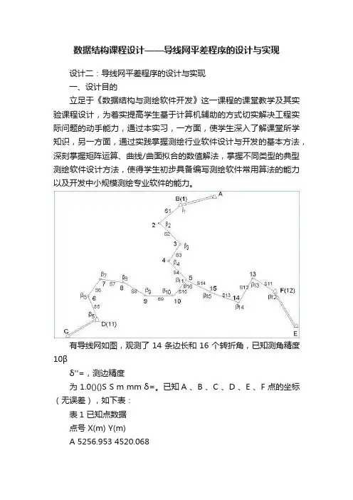
数据结构课程设计——导线网平差程序的设计与实现设计二：导线网平差程序的设计与实现一、设计目的立足于《数据结构与测绘软件开发》这一课程的课堂教学及其实验课程设计，为着实提高学生基于计算机辅助的方式切实解决工程实际问题的动手能力，通过本实习，一方面，使学生深入了解课堂所学知识，另一方面，通过实践掌握测绘行业软件设计与开发的基本方法，深刻掌握矩阵运算、曲线/曲面拟合的数值解法，掌握不同类型的典型测绘软件设计方法，使得学生初步具备编写测绘软件常用算法的能力以及开发中小规模测绘专业软件的能力。

有导线网如图，观测了14条边长和16个转折角，已知测角精度10βδ''=，测边精度为1.0()()S S m mm δ=。

已知A 、B 、C 、D 、E 、F 点的坐标（无误差），如下表：表1 已知点数据点号 X(m) Y(m)A 5256.953 4520.068B 5163.752 4281.277C 3659.371 3621.210D 4119.879 3891.607E 4581.150 5345.292F 4851.5545316.953表2 角度观测值编号角度观测值（° ′ ″）编号角度观测值（° ′ ″）1 163 45 04 9 169 10 302 64 58 37 10 98 22 043 250 18 11 11 94 53 50 4 103 57 34 12 111 14 235 83 08 05 13 79 20 18三、关键问题描述3.1 未知点近似坐标计算平面控制网进行平差计算时需要计算未知点的近似坐标1.坐标计算公式1、2点的坐标已知，并观测了1-2、1-3的夹角，根据这些数据可以求出3号点坐标根据1、2两点的坐标，可以反算出1、2方向的方位角T12,3号点的坐标为++=++=)sin()cos(121313121313ααT S y y T S x x式子中S13为观测边长，α为观测角度 2.计算流程从读入的数据循环计算未知点的坐标，已计算出的坐标当做已知坐标的点处理参加下次计算，以此类推，逐步计算出未知点的坐标3.实现算法CMatrix CPlaneNetAdjust::XYJS() { CMatrix _XYJS(Pnumber,2); double T12; for(int i=0;i0&&xy[k2].Y>0) { T12=GetT12(k1,k2); } double s12=Gets12(k1,k2); double s13=Gets12(k1,k3); double T13=T12+guancejiao[i].Guancezhi; double dx=s13*cos(T13); double dy=s13*sin(T13); xy[k3].X=xy[k1].X+dx; xy[k3].Y=xy[k1].Y+dy; } for(int i=0;i<="" bdsfid="103" double="" p="" temp1="xy[i].X;" temp2="xy[i].Y;" {="">}return _XYJS;}3.2 误差方程列立1.理论分析平面控制网的误差方程都是非线性方程，必须引入参数近似值将误差方程线性化，取X的充分近似值 0X ，x ?是微小量，在按台劳公式展开时可以略去二次和二次以上的项，而只取至一次项，于是可对非线性平差值观测方程式线性化，于是有如下的式子对于观测角的改正数有对于边长观测值的改正数有2.实现算法如下：CMatrix CPlaneNetAdjust::B() { CMatrix _B1(Lnumber,Pnumber*2); double a; double b; double c; double d; double m; double n; double m1; double n1; for(int i=0;i<="">D A D A D B D B DA DB X X Y Y X X Y Y L ??arctan ??arctan 1-----=-=αα()()22??S AD A D Y Y X X -+-=kjkjk k jk jk j jk jkj jk jk jk y S Y x S Y y S X x S Y ?)(?)(?)(?)(?200200200200"??+??-??-??+=ρρρραδh jhjh h jh jh j jh jh j jh jh jh y S Y x S Y y S X x S Y ?)(?)(?)(?)(?200 200200200"??+??-??-??+=ρρρραδ)(?)("?)("?)("?)("?)("?)("?)(" )("00200200200200200200200200i jk jh h jh jhh jh jh j jh jh j jh jh k jk jkk jk jk j jk jk j jk jk i L y S X x S Y y S X x S Y y S X x S Y y S X xS Y v ---??+?-?-?-+?-?-?-=ααρρρρρρρρi k jkjkk jk jk j jk jk j jk jk i l y S Y x S X y S Y x S X v -?+?+?-?-=000000000jki i S L l -=2002000)()(j k j k jk Y Y X X S -+-=_B1.setValue(i,2*k1,0);_B1.setValue(i,2*k1+1,0);}else{_B1.setValue(i,2*k1,a);_B1.setValue(i,2*k1+1,b);}if(k2<knpnumber)< bdsfid="148" p=""></knpnumber)<> {_B1.setValue(i,2*k2,0);_B1.setValue(i,2*k2+1,0);}else{_B1.setValue(i,2*k2,-a);_B1.setValue(i,2*k2+1,-b);}}for(int i=0;i<tnumber;i++)< bdsfid="160" p=""></tnumber;i++)<>{const double p=206.265;int k1=cezhan[i];int k3=huoshi[i];int k2=qianshi[i];double dx12=xy[k2].X-xy[k1].X;double dy12=xy[k2].Y-xy[k1].Y;double dx13=xy[k3].X-xy[k1].X;double dy13=xy[k3].Y-xy[k1].Y;c=(p*dx13/Gets12(k1,k3)/Gets12(k1,k3)-p*dx12/Gets12(k1,k2)/Gets12(k1,k2));c=-c;d=-p*dy13/Gets12(k1,k3)/Gets12(k1,k3)+p*dy12/Gets12(k1,k2)/Get s12(k1,k2);d=-d;m=-p*dy13/Gets12(k1,k3)/Gets12(k1,k3);m=-m;n=p*dx13/Gets12(k1,k3)/Gets12(k1,k3);n=-n;m1=p*dy12/Gets12(k1,k2)/Gets12(k1,k2);m1=-m1;n1=-p*dx12/Gets12(k1,k2)/Gets12(k1,k2);n1=-n1;if(k1<knpnumber)< bdsfid="183" p=""></knpnumber)<> {_B1.setValue(i+Snumber,2*k1,0);_B1.setValue(i+Snumber,2*k1+1,0);}else if(k1>=knPnumber){_B1.setValue(i+Snumber,2*k1,c);_B1.setValue(i+Snumber,2*k1+1,d);}if(k2<knpnumber)< bdsfid="194" p=""></knpnumber)<> {_B1.setValue(i+Snumber,2*k2,0);_B1.setValue(i+Snumber,2*k2+1,0);}else if(k2>=knPnumber){ _B1.setValue(i+Snumber,2*k2,m1); _B1.setValue(i+Snumber,2*k2+1,n1); } if(k3=knPnumber) { _B1.setValue(i+Snumber,2*k3,m); _B1.setValue(i+Snumber,2*k3+1,n); } }CMatrix _B(Lnumber,2*(Pnumber-knPnumber)); for(int i=0;i<_B1.getRow();i++) { for(int j=2*knPnumber;j<2*Pnumber;j++) { double temp=_B1.getValue(i,j); _B.setValue(i,(j-2*knPnumber),temp); } } return _B;}3.3 法方程构建与解算1.理论分析误差方程系数构成法方程2.实现代码①计算LCMatrix CPlaneNetAdjust::L() { CMatrix _L(Lnumber,1); double l; double s; double s0; for(int i=0;i<="" bdsfid="209" const="" cout<<l<l x B V -=?0?=-Pl B x PB B TTmin =PV V T V L L +=?20σ20?σPV V T double A13; double A;int k1=cezhan[i]; int k2=huoshi[i]; int k3=qianshi[i];A12=GetT12(k1,k2); A13=GetT12(k1,k3); A=GetA(k1,k2,k3); l=A13-A12; if(l<0) { l=pi+l; }if(l>=pi) { l=l-pi; }l=l-A;//cout<<rad_dms(a12)<<" "<<rad_dms(a)<<"<="" "<<rad_dms(a13)<<"="" bdsfid="220" p=""></rad_dms(a12)<<">"<<rad_dms(l)<<endl;< bdsfid="222" p=""></rad_dms(l)<<endl;<>_L.setValue(i+Snumber,0,rad_dms(l));} return _L; }②计算权阵PCMatrix CPlaneNetAdjust::P() { CMatrix _P(Lnumber,Lnumber); for(int i=0;i<="" p="" {="">temp=temp=Cjwucha*Cjwucha/(1*sqrt(bianchang[i].Len))/( 1*sqrt(bianchang[i].Len)); _P.setValue(i,i,temp); } for(int i=Snumber;i<="">3.4 精度估计1.单位权中误差间接平差与条件平差虽采用了不同的函数模型，但它们是在相同的最小乘原理下进行的，所以两法的平差结果总是相等的，这是因为在满足条件下的V 是唯一确定的，故平差值不因方法不同而异。

x0=[-0.004;86.806;14.846;25.706;31.216;42.626];
%------------------从文本框输入数据-------------------------------
%m=get(findobj('tag','edit1'),'string');
%l1=str2num(m);
七、MATLAB程序代码
1、经典自由网平差
[f,p1]=uigetfile('*.txt','选择高差文件')
fnal=strcat(p1,f);fpath=p1;
fm=fopen(fnal,'r');
while (~feof(fm))
l1=fscanf(fm,'%f',inf);
end
[f,p1]=uigetfile('*.txt','选择距离文件')
（3-2）
其中
(3-3)
(3-4)
得出
（3-5）
求得参数 的最佳估值为
参数 的协因数阵为
六、综合分析
从结果中我们可以看出，三种平差方法所得高差的改正数是相同的，所得参数 的最佳估值是不同的。
经典自由网平差适用于起算数据充足的情况，而秩亏自由网平差适用于起算数据不足，需要加一个基准条件才能进行平差计算。拟稳平差则是选择一些相对稳定的点进行平差，是那些不稳定的点不参与平差。根据实际情况我们选择适宜的平差方法。
%s=str2num(n);
%s=s';
%------------------从文本框输入数据--------------------------------------------

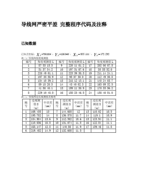
导线网严密平差 完整程序代码及注释已知数据已知点坐标：XA=730.024 ，YA=126.040 ，111.855=XB，232.172=Y B应得结果 = 5.30表七：实际结果点号X(m) Y(m) 中误差X(mm) 中误差Y(mm) 点位中误差1 678.1641 287.3411 3.3868 5.8737 7.60782 564.6919 446.8827 6.0102 7.5137 9.19373 533.8468 629.2749 8.7985 7.3927 10.05964 475.6776 535.8728 7.3949 8.4987 9.96675 499.1408 374.4231 5.8076 7.6840 9.18276 594.6190 176.7976 5.2308 3.4068 7.34757 826.3848 305.7569 2.7439 5.4473 7.15518 767.8778 401.8510 4.8371 6.3810 8.37349 745.7230 531.0410 6.8992 6.6276 9.194710 671.6256 650.8637 9.0695 6.0533 9.722011 794.2833 600.4688 8.4994 6.1800 9.578412 859.0528 511.5349 6.7399 6.6874 9.160813 898.2695 399.0763 4.7580 6.4207 8.358614 919.3459 276.9409 3.1903 4.8006 7.0670单位权中误差： 5.3393详细代码% 贡XX导线严密平差程序clear;clc;% 从文件中输入数据% S1 观测角度数据% 【角号度分秒左点角点右点】-1为已知点B，0为已知点A fid1=fopen('S1.txt','rt');[S1,~]=fscanf(fid1,'%f ',[7 24]);fclose(fid1);S1=S1';% S2 边长观测值% 【边号距离测边中误差对应角号】fid2=fopen('S2.txt','rt');[S2,~]=fscanf(fid2,'%f ',[5 17]);fclose(fid2);S2=S2';% S3：度分秒到角度[S3]=dfm2jd(S1);% 计算坐标近似值% X0=[x1 y1 x2 y2 ......][X0]=zbjs(S2,S3);% 循环，未知参数改正量最大值mx<0.01mm停止mx=100;while mx>0.01% 计算B，l，P 矩阵[B,l,P]=BBll(X0,S2,S1,S3);% P68页x=(B'*P*B)\B'*P*l;% 改正量mx=max(x);v=B*x+l;[rr,cc]=size(B);m0=sqrt((v'*P*v)/(rr-cc));% 单位权中误差Q=inv(B'*P*B);% 协因数阵M=m0^2*Q;% 未知数方差矩阵% 平差后坐标X=X0'+x/1000;X0=X';end% 坐标中误差for i=1:28det(i)=sqrt(M(i,i));end% 点位中误差for i=1:14ddet(i)=2.5*sqrt(det(i*2-1)+det(i*2));endddet=ddet';% 整理数据，输出最终结果for i=1:14XX(i,1)=X(2*i-1);XX(i,2)=X(2*i);DD(i,1)=det(2*i-1);DD(i,2)=det(2*i);endjieguo(:,1)=1:14;jieguo(:,2)=XX(:,1);jieguo(:,3)=XX(:,2);jieguo(:,4)=DD(:,1);jieguo(:,5)=DD(:,2);jieguo(:,6)=ddet;disp('计算完成！')fid=fopen('输出结果.txt','wt');fprintf(fid,'点号 X(m) Y(m) 中误差X(mm) 中误差Y(mm) 点位中误差 \n');fprintf(fid,' %2d %11.4f %11.4f %5.4f %5.4f %5.4f\ n',(jieguo)');fprintf(fid,'单位权中误差：%8.4f',(m0)');fclose(fid);====================================================% 单位转换function [S3]=dfm2jd(S1)for i=1:24S3(i,1)=S1(i,1);S3(i,2)=(S1(i,2)+S1(i,3)/60+S1(i,4)/3600);End====================================================% 计算坐标近似值function [X0]=zbjs(S2,S3)% 起始数据X10=[730.024;126.040;855.111;172.232];X0=zeros(1,28);% 预分配内存% 已知边方位角t=180+atand((X10(2)-X10(4))/(X10(1)-X10(3)));% 下方闭合% 起始方位角t1=t;for i=1:1:6% 计算各边方位角if S2(i,5)>0 % i=4t1=t1+S3(S2(i,4),2)+S3(S2(i,5),2)-180;% 边4方位角+角6+角7-180 elset1=t1+S3(S2(i,4),2)-180;endif t1<0t1=t1+360;end% 计算各点近似坐标if i<2X0(1)=X10(1)+S2(1,2)*cosd(t1);X0(2)=X10(2)+S2(1,2)*sind(t1);endif i>=2X0(2*i-1)=X0(2*(i-1)-1)+S2(i,2)*cosd(t1);X0(2*i)=X0(2*(i-1))+S2(i,2)*sind(t1);endend% 上方闭合% 起始方位角t2=t;t2=t2-S3(12,2);if t2<0t2=t2+360;endfor i=8:1:15% 计算个边方位角if i<9 % i=8X0(2*(i-1)-1)=X10(3)+S2(i,2)*cosd(t2);X0(2*(i-1))=X10(4)+S2(i,2)*sind(t2);endif i>8t2=t2+S3(S2(i,4),2)-180;if t2<0t2=t2+360;end% 计算各点近似坐标X0(2*(i-1)-1)=X0(2*(i-2)-1)+S2(i,2)*cosd(t2); X0(2*(i-1))=X0(2*(i-2))+S2(i,2)*sind(t2);endend==================================================== % 计算方位角function [M]=fangweijiao(a,b,X0)X10=[730.024;126.040;855.111;172.232];% 确定边对应两点类型及坐标。

B L2
L1 A
L3 C
9
clc Disp(‘条件平差示例２’) Disp(‘三角形内角观测值’) L1 = [42 12 20] L2 = [78 9 9] L3 = [59 38 40] L = [L1; L2; L3] Disp(‘将角度单位由度分秒转换为弧度’) LL = dms2rad(mat2dms(L))
设误差Δ和参数X的估计值分别为V 和 Xˆ
15
则有
V AXˆ l
为了便于计算，通常给参数估计一个充分接近的近似值 X 0
Xˆ X 0 xˆ 则误差方程表示为
V Axˆ l
其中常数项为
l L (AX 0 d)
16
由最小二乘准则，所求参数的改正数应该满足
V T PV min
目标函数对x求一阶导数，并令其为零
if(sum(LL) == pi) disp(‘检核正确’)
else
V = A'*Ka
disp(‘检核错误’) end
11 例 《误差理论与测量平差基础》P75
在下图中，Ａ、Ｂ为已知水准点，其高程为 HA=12.013m, HB = 10.013m, 可视为无误差。为 了确定点Ｃ及Ｄ点的高程，共观测了四个高差，高差 观测值及相应的水准路线的距离为：
disp(‘系数矩阵B’)
B = [1 0; 0 1; 1 0; 0 1; -1 1; -1 0]
l = [0; 0; 4; 3; 7; 2]
disp(‘C是单位权观测高差的线路公里数，S是线路长度’)
C = l*ones(1,6)
23
h6
E h3
h7 B
S = [1.1, 1.7, 2.3, 2.7, 2.4, 4.0]

用MATLAB解决_条件平差和间接平差测量程序设计条件平差和间接平差一、条件平差基本原理A LA0函数模型 A VW0r n n 1 r 1r 12 21随机模型D? Q? P0 0TV P Vm i n平差准则条件平差就是在满足r个条件方程式条件下,求使函数V‘PV最小的V值,满足此条件极值问题用拉格朗日乘法可以求出满足条件的V值。

?A LA01、平差值条件方程: 0r n n 1r 1r 1a La L a La01 12 2 n n 0b Lb L b Lb01 12 2 n n 0?r Lr L r Lr01 12 2 n n 0a ,b ,, r i1 , 2 ,, n 条件方程系数i i ia ,b ,, r0 0 0常数项?A LA02、条件方程: 0r n n 1r 1r 1将LLV代入平差值条件方程中,得到A VW0r 1 n 1 r 1 r 1w , w ,, wa b r为条件方程闭合差WA LA闭合差等于观测值减去其应有值。

3、改正数方程:按求函数条件极值的方法引入常数TK k , k ,, ka b rr 1称为联系系数向量,组成新的函数:T T? V P V2 K A VW将Ω对V求一阶导数并令其为零?T T2 V P2 K A0VT1 T TP VA K则: VP A KQ A K4、法方程: 将条件方程 AV+W0代入到改正数方程VQATK 中,则得到:TA Q A KW0N KW0记作: a ar 1 r 1 r 1r rTR N R A Q A R A r由于 a a1 T1K? N W? A Q A A LANaa为满秩方阵,a a 0TLLVVQ A K按条件平差求平差值计算步骤A VW01、列出rn-t个条件方程r 1 n 1 r 1 r 1T1 TN KW0NA Q AA P A2、组成法方程a aa ar 1 r 1 r 1r r1K? N Wa a3、求解联系系数向量4、将 K值代入改正数方程VP-1ATKQATk中,求出V值,并求出平差值LL+V。

序。Ｍ Ａ Ｔ Ｌ Ａ Ｂ与 其 他 算 法 语 言相 比 ， 具有编程简单 、 运 算速 度 快 的 特 点 ， 特 别 是 在 矩 阵运 算 方 面 ， 在 最 小 二 乘
平 差 中可 以发 挥 很 好 的作 用 ， 能 大 大 提 高 工 程 测 量 中 的数 据处 理 效 率 。 关键 词 ： 平 差； Ｍ Ａ Ｔ Ｌ Ａ Ｂ优 化 箱 ； 附 线 性 不 等 式 约 束
２ ０ １ ３年第 ７ 期
中州 煤炭
总第 ２ １ １ 期
基 于 ＭＡＴ Ｌ Ａ Ｂ 的 测 量 平 差 计 算
高 思培 ， 陈冠 宇 ， 范新 华 ， 王 耀鑫 ， 王强昆
（ １ ， 河 南理 工 大 学 测绘 与 国 土 信 息 工 程 学 院 ， 河 南 焦作 ２ ． 桂林理 工大学 测绘地理信 息学院， 广西 桂林 ４ ５ ４ ０ ０ ０ ； ７ １ ０ ０ ４ ３ ） ５ ４ １ ０ ０ ６ ； ３ ． 机械工业勘察设计研 究院， 陕西 西安
＝
（ 胎 ） Ｂ Ｐ １ ， Ｐ为 观测 值 的权 阵。
平差值 向量 的协 因数阵 ：
Ｑ Ｌ Ｌ＝ Ｂ（ 曰 Ｐ Ｚ ） 曰
计 算 软件 ， 它 以矩 阵 运算 为基 础 ， 把计算 、 绘 图及 动 态 系统 仿真 等功 能有 机 融合在 一起 。ＭＡ Ｔ Ｌ Ａ Ｂ将 高 性 能 的数值 和符 号计 算功 能 、 强 大 的绘 图功 能 、 程 序 语 言设 计功 能 以及为 数众 多 的应用 工具 箱集 成在 一
Ｈ ａ＝ ２ ３ ７ ． ４ ８ ３ ｍ， 为求 Ｂ、 Ｃ、 Ｄ三点 的高 程 ， 进 行 了水
准测 量 ， 其结果 见表 １ ， 试 按 间 接 平 差 求 定 Ｂ、 Ｃ 、 Ｄ

a）绘制三维圆柱螺旋线， ，要求给出相应的坐标轴和标题附加标注，螺旋线为蓝色虚线。
在matlab中，有一种特殊的运算，因为其运算苻是在有关算术运算苻前面加点，因此叫点运算。点运算苻有.*,./,.\和.^。两个矩阵进行点运算是指它们的对应元素进行相关运算，要求两矩阵的维参数相同。
三、实验仪器和设备
1.计算机1台
四、预习要求
1．复习特殊矩阵的产生。
2．复习矩阵的加减乘除与乘方运算，以及相应的点运算。
（1）求它们的乘积C；
（2）将矩阵C的右下角3*2子矩阵赋给D；
（3）察看matlab工作空间的使用情况。
六、实验报告要求
实验报告应包括实验目的、实验内容、流程图、程序清单、运行结果以及实验的收获与体会。
实验二、
一、实验目的
1，掌握生成特殊矩阵的方法；
2，掌握矩阵分析的方法；
3，用矩阵求逆法求解线性方程组。
5，完成以下各题，将答案写入实验报告，并在机器上运行结果验证
（1）编写一个函数文件求两个数的最大值。
（2）编写一个函数文件求三个数的最大值。
（3）编写一个函数文件，求矩阵的最大元
（4）编写一个函数文件，以向量为参数，对向量元素进行排序并输出
六、实验报告要求
1.完成实验内容中的计算；
2.验证实验内容中计算所得结果的正确性。
（3）try语句
3）循环结构
（1）for语句
（2）while语句
（3）break语句与continue语句
（4）循环的嵌套
3，函数文件
function 输出形参表＝函数名（输入形参表）
注释说明部分
函数体语句
三、实验仪器和设备
1.计算机1台
四、预习要求

A h2 D h1
C h6 E h3 h5 h7 B h4
disp(‘C是单位权观测高差的线路公里数，S是线路长度’) 是单位权观测高差的线路公里数， 是线路长度 是线路长度’ 是单位权观测高差的线路公里数 C = l*ones(1,6)
S = [1.1, 1.7, 2.3, 2.7, 2.4, 4.0] P = C./S % 定义观测值的权， 定义观测值的权， P = diag(P) % 定义权阵 disp(‘参数的解’) 参数的解’ 参数的解 x = inv(B’*P*B)*B’*P*l disp(‘误差 误差V(mm), 各待定点的高程平差值 （m）’) 各待定点的高程平差值L1（ ） 误差 V = B*x - l % 误差方程 误差方程(mm) L1 = L + V/1000 % 观测值的平差值， 观测值的平差值， disp(‘精度评定’) 精度评定’ 精度评定 n = 6; % 观测值的个数 t = 2; % 必要观测数 delta = sqrt(V’*P*V/(n – t))
H(1,1)+H(2,1)-H(3,1)+HAH(2,1)if H(1,1)+H(2,1)-H(3,1)+HA-HB==0 && H(2,1)H(4,1)==0 disp(‘检核正确 检核正确') disp( 检核正确') else disp(‘检核错误 检核错误') disp( 检核错误') end disp(‘平差后的高程值 平差后的高程值') disp( 平差后的高程值') HC = HA + H(1,1) HD = HA + H(1,1) + H(4,1)
二、间接平差的基本原理
在一个控制网中，设有t个独立参数， 在一个控制网中，设有t个独立参数，将每一个观测值都表达 成所选参数的函数，以此为基础进行平差， 成所选参数的函数，以此为基础进行平差，最终求得参数的估 计值。 计值。 选择参数应做到足数（参数的个数等于必要观测数）和独 选择参数应做到足数（参数的个数等于必要观测数） 参数间不存在函数关系）。 ）。利用参数将观测值表示为 立（参数间不存在函数关系）。利用参数将观测值表示为

表 ３ 边数 据 结 构
Ｔａ ． Ｄ ｔ ｔｕ ｔ ｒ ｎ ｓ ｌ ３ ａ ａ ｓｒ ｃ ｕ ｅ ｏ ｌ ｅ ｂ ｆ ｉ
广泛． 常情况 下 ， 外 业 观测 数 据 量 大 ， 据处 理 通 其 数 过程 中大多涉及 到矩 阵 的计 算 ， 由于 导 线 网 网形 且 的不确定 性 ， 因此其 程序设 计 非常 复 杂［． 文总结 １本 ］ 导线 网的规律 ， 计 出通 用数据 结 构 ， 设 并基 于 Ｍａｌ ｔｂ ａ 强大的矩阵计 算能力 ， 编制 了导线网数据处理 程序．
表 １ 点 表 数 据 结构
Ｔ ｂ Ｄａ ａ ｓ １ ｔ Ｉ ｆｐ ｉ ｔ ａ ．１ ｔ ｈ ｌ ｌ ℃ｏ ｏ ｎ ｓ ｃｌ
表 １３中分 别存 储在 ｐＴａ ，ｉｅ ａ ，ｎ ｌＴ ｂ － ｔ ｂ ｌ Ｔ ｂａ ｇｅ ａ ｎ 矩阵中， 保存为． ａ 文件 ， ｍｔ 程序运行时加载嘲．
传 递 到网 中每一条 边． 某角 度一 边方 位 已知 ， 设 而另
一
边方 位未 知 ， 由于两边 夹角 已知 ， 可计 算 出未知 边
表 ２ 角 度 数 据 结 构
ａ ． ａ ａ ｓｒ ｃｕ ｅ ｏ ｎ ｌｓ Ｔ ｂ ２ Ｄ ｔ ｔ ｕ ｔ ｒ ｆａ ｇｅ
的方位 ． １ 示 为 ４种 可能 情况 ． 图 所
一 ±７ 口 ｃ － ４
函数迭代计算．
ｅｄ ｎ
ｅｄ ｎ
情 况 四 ： ＝ ． ４ ７ ａ ． ， ＝厂 ＝ －ｃ － ４
（） ４
同理可得 ， 已知右边方位角计算左边方位角 的 情 况 ， 有 ４ 可 能性． 也 种 程序 根据 角度 两边 的端 点点
名 的关 系判断 以上 ８种 情 况 ， 用 相 应 的计 算 公 式 采 计算 未 知边方 位角 ［． ３ ］ 程 序在 获 得 未知 边 方 位 角后 ， 计 算 结果 保 存 将 到边表相 应记 录 中． 然后 在角 度 表 中搜 索相 邻角 度 ，

function BJPC2ZB=[];ZJ=[];BC=[];%%format long[filename,filepath]=uigetfile('*.txt','选择平差文件:'); name=[filepath filename];fid1=fopen(name,'rt');if(fid1==-1)disp('文件未打开，请重试！');return;endn=fscanf(fid1,'%f',1);%输入边的个数b=fscanf(fid1,'%f',1);%输入多余观测个数E=fscanf(fid1,'%f',1);%输入测角中误差t=fscanf(fid1,'%f',1);%输入坐标个数ZB=fscanf(fid1,'%f',[2 t]);dms1=fscanf(fid1,'%f',[3 n+1]);BC=fscanf(fid1,'%f',[1 n]);T0=fscanf(fid1,'%f',1);T1=fscanf(fid1,'%f',1);fclose(fid1);dms=dms1';ZJ=dms2degrees(dms);%%if t==2T0=T0;%若告诉起始方位角就直接输入endif t==4 %若没有告诉起始方位角由坐标反算Xa=ZB(1,1);Xb=ZB(1,2);Ya=ZB(2,1);Yb=ZB(2,2);Tx=Xb-Xa; Ty=Yb-Ya;T0=atan(Ty/Tx)*180/pi;%对方位角的讨论if ((Tx>0)&&(Ty>0))T0;endif (((Tx<0)&&(Ty>0))||((Tx<0)&&(Ty<0)))T0=T0+180;endif ((Tx>0)&&(Ty<0))T0=T0+360;endif ((Tx==0)&&(Ty>0))T0=90;endif ((Tx==0)&&(Ty<0))T0=270;endif((Ty==0)&&(Tx>0))T0=0;endif ((Ty==0)&&(Tx<0))T0=180;endenda0=T0;x0=ZB(1,t/2);y0=ZB(2,t/2);A=[0,0];FWJ=[];%开始计算近似方位角J=1;while(J<=n+1)belta=ZJ(J);%讨论方位角if J==1a=a0+belta;elsea=a+belta;endif a>=180a=a-180;elsea=a+180;endif a>=360a=a-360;endFWJ(J)=a;J=J+1;endFWJ;%%J=1;%开始计算近似坐标Awhile(J<=n)if J==1A(1,1)=x0+BC(1)*cos(FWJ(1)*pi/180);A(2,1)=y0+BC(1)*sin(FWJ(1)*pi/180);elseA(1,J)=A(1,J-1)+BC(J)*cos(FWJ(J)*pi/180); A(2,J)=A(2,J-1)+BC(J)*sin(FWJ(J)*pi/180);endJ=J+1;endA;%%W=[];%开始计算闭合差if t==2T1=T1;endif t==4Xa=ZB(1,3);Xb=ZB(1,4);Ya=ZB(2,3);Yb=ZB(2,4);Tx=Xb-Xa; Ty=Yb-Ya;T1=atan(Ty/Tx)*180/pi;if ((Tx>0)&&(Ty>0))T1;endif (((Tx<0)&&(Ty>0))||((Tx<0)&&(Ty<0)))T1=T1+180;endif ((Tx>0)&&(Ty<0))T1=T1+360;endif ((Tx==0)&&(Ty>0))T1=90;endif ((Tx==0)&&(Ty<0))T1=270;endif((Ty==0)&&(Tx>0))T1=0;endif ((Ty==0)&&(Tx<0))T1=180;endendW(1,1)=-(FWJ(n+1)-T1)*3600;%以秒为单位W(2,1)=-(A(1,n)-ZB(1,t/2+1))*100;%以厘米为单位W(3,1)=-(A(2,n)-ZB(2,t/2+1))*100;W;%%XS=zeros(3,2*n+1);%开始计算系数阵，XS是系数阵e=n+1;while(e<=2*n+1)XS(1,e)=1;e=e+1;endf=1;while(f<=n)XS(2,f)=cos(FWJ(f)*pi/180);%纵坐标边长改正数的系数 XS(3,f)=sin(FWJ(f)*pi/180);%横坐标边长改正数的系数 f=f+1;endu=1;y0=A(2,n);x0=A(1,n);Y=[];X=[];y1=[];x1=[];while(u<=n+1)if u==1Y(1)=ZB(2,t/2);X(1)=ZB(1,t/2);elseY(u)=A(2,u-1);X(u)=A(1,u-1);endu=u+1;endy1=-1/2062.65*(y0-Y);%纵坐标转角改正数的系数x1=1/2062.65*(x0-X);%横坐标转角改正数的系数y1;x1;d=n+1;z=1;while(d<=2*n+1)XS(2,d)=y1(1,z);XS(3,d)=x1(1,z);d=d+1;z=z+1;endXS;%%r=[];h=1;while (h<=n)s=(5+5*BC(h)/1000)/10;%求中误差厘米为单位r(h)=E^2/s^2;%计算距离的权h=h+1;endaa=[];y=1;while(y<=n)aa(y)=r(y);%将距离的权赋给矩阵aay=y+1;endc=n+1;while(c<=2*n+1)aa(c)=1;%转角的权都是1c=c+1;endP=diag(aa);%形成权阵P;%%Q=inv(P);N=XS*Q*XS';N1=inv(N);K=inv(N)*W;V=Q*XS'*K;V;BC1=BC'+V(1:n)/100;%将改正数加到观测值以求平差边长（除一百统一单位）ZJ1=ZJ+V(n+1:2*n+1)/3600;%同上BC1;i=1;while (i<=n+1)ZJ2(i,1)=fix(ZJ(i));ZJ2(i,2)=fix((ZJ(i)-fix(ZJ(i)))*60);ZJ2(i,3)=((ZJ(i)-fix(ZJ(i)))*60-fix((ZJ(i)-fix(ZJ(i)))*60))*60;i=i+1;endZJ2;%%A1=[0,0];FWJ1=[];J=1;while(J<=n+1)belta=ZJ1(J);if J==1a=a0+belta;elsea=a+belta;endif a>=180a=a-180;elsea=a+180;endif a>=360a=a-360;endFWJ1(J)=a;J=J+1;endi=1;while (i<=n+1)FWJ3(i,1)=fix(FWJ(i));FWJ3(i,2)=fix((FWJ(i)-fix(FWJ(i)))*60);FWJ3(i,3)=((FWJ(i)-fix(FWJ(i)))*60-fix((FWJ(i)-fix(FWJ(i)))*60))*60;FWJ2(i,1)=fix(FWJ1(i));FWJ2(i,2)=fix((FWJ1(i)-fix(FWJ1(i)))*60);FWJ2(i,3)=((FWJ1(i)-fix(FWJ1(i)))*60-fix((FWJ1(i)-fix(FWJ1(i)))*60))*60; i=i+1;endFWJ3;FWJ2;%%J=1;%开始计算平差坐标A1while(J<=n)if J==1A1(1,1)=ZB(1,t/2)+BC1(1)*cos(FWJ1(1)*pi/180);A1(2,1)=ZB(2,t/2)+BC1(1)*sin(FWJ1(1)*pi/180);elseA1(1,J)=A1(1,J-1)+BC1(J)*cos(FWJ1(J)*pi/180);A1(2,J)=A1(2,J-1)+BC1(J)*sin(FWJ1(J)*pi/180);endJ=J+1;endA1;m=sqrt(V'*P*V/b);%测量精度单位权中误差。

function [zjbl1 kp ukp sp sa ss pn pn1 rlf12 x y x1 y1 k1 k2 k3 ma ms1 ms2 angles zjbl2 k11 k22 s]=readdata;global zjbl1 kp ukp sp sa ss pn pn1 rlf12 x y x1 y1 k1 k2 k3 ma ms1 ms2 angles zjbl2 k11 k22 s;[filename,pathname]=uigetfile('*.dat;*.txt','¶ÁÈ¡Êý¾Ý');if filename~=0[fid1 msg]=fopen(strcat(pathname,filename),'rt');if fid1>0kp=fscanf(fid1,'%f',1);ukp=fscanf(fid1,'%f',1);sp=kp+ukp;sa=fscanf(fid1,'%f',1);ss=fscanf(fid1,'%f',1);pn=fscanf(fid1,'%s',[1 sp]);pn1=pn;rlf12=fscanf(fid1,'%f',2);rlf12=de_to_rad(rlf12);x=fscanf(fid1,'%f',1);y=fscanf(fid1,'%f',1);x1=zeros(1,2);x1(2)=x(1);y1=zeros(1,2);y1(2)=y(1);ma=fscanf(fid1,'%f',1);ms1=fscanf(fid1,'%f',1);ms2=fscanf(fid1,'%f',1);zjbl1=fscanf(fid1,'%s%s%s%f',[4 sa]); %Öмä±äÁ¿zjbl1=zjbl1';k1=zjbl1(:,1);k2=zjbl1(:,2);k3=zjbl1(:,3);angles=zjbl1(:,4);angles=de_to_rad(angles);zjbl2=fscanf(fid1,'%s%s%f',[3 ss]); %Öмä±äÁ¿zjbl2=zjbl2';k11=zjbl2(:,1);k22=zjbl2(:,2);s=zjbl2(:,3);fclose(fid1);k1=chkdat(sp,pn,k1);k2=chkdat(sp,pn,k2);k3=chkdat(sp,pn,k3);k11=chkdat(sp,pn,k11);k22=chkdat(sp,pn,k22);x1(1)=x1(2)-s(1)*cos(rlf12(1));y1(1)=y1(2)-s(1)*sin(rlf12(1));elseerror(msg);endendfunction [x1 y1]=calculatex0y0(ukp,rlf12,angles,k1,x1,y1,s)for i=1:ukpif i==1rlf(i)=rlf12(1)+rlf12(2)-pi;elserlf(i)=rlf(i-1)+angles(i)-pi;endif rlf(i)<0rlf(i)=rlf(i)+2*pi;elseif rlf(i)>2*pirlf(i)=rlf(i)-2*pi;elserlf(i)=rlf(i);endx1(k1(i+1))=x1(k1(i))+s(i)*cos(rlf(i));y1(k1(i+1))=y1(k1(i))+s(i)*sin(rlf(i));endfunction [B L]=calculatebl(sa,ss,s,sp,x1,y1,k1,k2,k11,k22,k3,kp,angles); B=(zeros(sa+ss,sp*2));p=206264.80624709;for i=1:sadetx1=x1(k2(i))-x1(k1(i));dety1=y1(k2(i))-y1(k1(i));s1=solvedis(x1(k1(i)),x1(k2(i)),y1(k1(i)),y1(k2(i)));T1=fangweijiao(x1(k1(i)),x1(k2(i)),y1(k1(i)),y1(k2(i)));detx2=x1(k3(i))-x1(k1(i));dety2=y1(k3(i))-y1(k1(i));s2=solvedis(x1(k1(i)),x1(k3(i)),y1(k1(i)),y1(k3(i)));T2=fangweijiao(x1(k1(i)),x1(k3(i)),y1(k1(i)),y1(k3(i)));B(i,2*k1(i)-1)=p*(dety1/(s1^2)-dety2/(s2^2));B(i,2*k1(i))=-p*(detx1/(s1^2)-detx2/(s2^2));B(i,2*k2(i)-1)=-p*(dety1/(s1^2));B(i,2*k2(i))=p*(detx1/(s1^2));B(i,2*k3(i)-1)=p*(dety2/(s2^2));B(i,2*k3(i))=-p*(detx2/(s2^2));if k1(i)<=kpB(i,2*k1(i)-1)=0;B(i,2*k1(i))=0;endif k2(i)<=kpB(i,2*k2(i)-1)=0;B(i,2*k2(i))=0;endif k3(i)<=kpB(i,2*k3(i)-1)=0;B(i,2*k3(i))=0;endT(i)=T1-T2;if T(i)<0T(i)=T(i)+2*pi;elseif T(i)>2*piT(i)=T(i)-2*pi;elseT(i)=T(i);endL(i)=(angles(i)-T(i))*206264.80624709;%ת»¯ÎªÃ뵥λ£»endfor ii=1:ssdetx11=x1(k22(ii))-x1(k11(ii));dety11=y1(k22(ii))-y1(k11(ii));s11=solvedis(x1(k11(ii)),x1(k22(ii)),y1(k11(ii)),y1(k22(ii))); s21(ii)=s11;B(sa+ii,2*k11(ii)-1)=-(detx11/(s11));B(sa+ii,2*k11(ii))=-(dety11/s11);B(sa+ii,2*k22(ii)-1)=(detx11/s11);B(sa+ii,2*k22(ii))=(dety11/s11);if k11(ii)<=kpB(ii+sa,2*k11(ii)-1)=0;B(ii+sa,2*k11(ii))=0;endif k22(ii)<=kpB(ii+sa,2*k22(ii)-1)=0;B(ii+sa,2*k22(ii))=0;endL(sa+ii)=s(ii)-s21(ii);endP=zeros(sa+ss,sa+ss);for i=1:saP(i,i)=1;endfor j=sa+1:sa+ssP(j,j)=ma^2/((ms1+ms2*s(j-sa)/1000)/1000)^2;endB=B(:,kp*2+1:sp*2);N=B'*P*B;W=B'*P*L';xy=inv(N)*W;v=B*xy-L';zwc=sqrt(v'*P*v/(ss+sa-ukp*2));%ÖÐÎó²îQxx=inv(N);DDDZwcxy=zwc*sqrt(diag(Qxx)); %´ý²âµãx¡¢yÖÐÎó²î£»for j=1:ukpxpc(kp+j)=x1(kp+j)+xy(2*j-1);ypc(kp+j)=y1(kp+j)+xy(2*j);DDDZwc(j)=sqrt(DDDZwcxy(j)^2+DDDZwcxy(j+1)^2);end[filename,pathname]=uiputfile('*.dat;*.txt','±£´æ');[fid2 msg]=fopen(strcat(pathname,filename),'w+');if fid2>0fprintf(fid2,'¡ª¡ª¡ª¡ª¡ª¡ª¡ª¡ª¡ª¡ª¡ª¡ªµ¼Ïßƽ²î½á¹û¡ª¡ª¡ª¡ª¡ª¡ª¡ª¡ª¡ª¡ª¡ª¡ª\n\n');fprintf(fid2,'µ¥Î»È¨ÖÐÎó²î=%8.1f¡±\n\n',zwc);for ii=1:ukpout1(ii)=pn1((kp+ii));endout=[x1(kp+1:sp)' y1(kp+1:sp)' xpc(kp+1:sp)' ypc(kp+1:sp)'1000*DDDZwc'];for k=1:ukpfprintf(fid2,'´ý¼ÆËãµ¼Ïßµã%c \n',out1(k));fprintf(fid2,'½üËÆ×ø±êx0/£¨m£© ½üËÆ×ø±êy0/£¨m£©Æ½²îºóx/£¨m£© ƽ²îºóy/£¨m£© µãλÖÐÎó²î/£¨mm£©\n');fprintf(fid2,'%10.3f%17.3f%15.3f%15.3f%15.1f\n\n',out(k,:));endfclose(fid2);elseerror(msg);endmsgbox('±£´æ³É¹¦£¡');。

创新实践报告实践名称：基于MATLAB测量平差程序设计系部名称：测绘工程学院专业班级：测绘工程11-6班学生姓名：学号：指导教师：xxx工程学院教务处制注：1、此报告为参考格式，各栏项目可根据实际情况进行调整；实验成绩以优（90~100）、良（80~89）、中（70~79）、及格（60~69）、不及格（60以下）五个等级评定。

附录1 外文参考文献原文参考文献一Improving oil fields recovery through real-time water flooding optimizationPamela Alessia Chiara MarescalcoPolitecnico di Torino, Land, Environment and GeoTechnologies Engineering Department,24, C.so Duca degli Abruzzi, 10129 Torino, ItalySUMMARYIncreasing oil recovery from reservoirs is a strong urge. One of the most effective ways to get the result iswater flooding and that’s why its application is nowadays widely used in the petroleum industry. Obviously,water flooding efficiency strongly depends on reservoir properties; this makes simulating a water injectionprocess a priori an extremely important step of the reservoir production strategy. Simulation is commonlydone adopting a finite difference (FD) simulation approach.This paper explores a different and complementary approach, represented by streamline-based simulation,coupled with a tool to optimize water flooding campaigns and to help quick decision making. Inthe present study, water flooding simulation is performed via two commercial software: an FD and astreamline-based simulator, to highlight advantages and disadvantages of both simulation techniques indescribing a water injection campaign and to exploit the two appr oaches’ uniqueness in parallel.The final goal of iteratively converging to the optimal water flooding scheme, which is the core of thepresent work, is achieved through a customized Matlab script. The generated automatic procedure showsits effectiveness in improving oil recovery, expediting decision making and saving time and FD simulationruns. A three steps workflow is outlined to get the best water flooding scheme for the examples shownbelow. Copyright q 2008 John Wiley & Sons, Ltd.Received 13 March 2008; Revised 1 September 2008; Accepted 8 November 2008KEY WORDS: water displacement optimization; FD simulation; streamline simulation; Matlab automatedroutine; real-time decision making; quantitative and iterative adjustment of water rates tobe injectedINTRODUCTIONIn the last decades water flooding has been widely applied in the petroleum field, both in mature and in newly developed fields, and its attractiveness lies in supporting the entire field pressureduring depletion and in improving the final oil recovery [1–3]. The techniqueconsists in injecting water with the purpose of displacing and therefore producing oil, especially if the reservoir lacks an underlying aquifer able to counterbalance the depletion and to drive oil to the producer wells.To really understand a water flooding process and to predict its efficiency, it is useful to simulate it a priori. This is usually done via finite difference (FD) simulation, which is able to describe any kind of existing reservoir very accurately, but unfortunately is not able to give enough details about the way the flow occurs throughout the field. Recent works [4, 5] have proposed a newly developed approach, based on streamline simulation, whose main attraction lies in providing information not obtainable from FD simulation and useful for the purpose of improving reservoir performances.In the present study, water flooding simulation is performed via two commercial software: an FDand a streamline-based simulator, to highlight advantages and disadvantages of both simulationtechniques in describing a water injection campaign and to exploit the two approaches’ uniquenessin parallel. If FD simulation is essential to checking the streamline simulation results, the streamlinebasedsimulator is, on the other hand, an ideal tool to perform a procedure able to optimizewater injection. Then, the core of the work and its innovative approach lies in exploiting the twosoftware features in conjunction with the application of a customized Matlab code developed inorder to elaborate all the streamline simulation outputs, to calculate the changes to be made to theproduction/injection constraints for the subsequent simulation run, so as to iteratively converge tothe optimal injection scheme for the reservoir under study. A three steps workflow is outlined toget the best water flooding scheme for the examples shown below.FD APPROACH VERSUS STREAMLINE SIMULATIONECLIPSE is a complete and complex simulator, whose attractiveness resides in being able todescribe any kind of reservoir, including geological complexity, formation features, and fluidproperties. The simulator is based on a time and spatial discretization and solves a three-dimensionalequation by assigning to all the parameters involved in the simulation a unique value, associated withthe entire cell, for every grid block. For models with a large number of cells, using FD relaxationcan be computationally heavy; therefore, a good balance must be kept between having sufficientaccuracy in describing the reservoir and keeping simulation time within reasonable limits [6].3DSL, on the other side, solves two different equations on two different grids and this is usuallyfaster than FD simulation, especially for large models: the pressure equation is solved implicitlyon the background grid (or pressure grid), whereas the saturation equation is solved explicitly onthe streamline grid. This involves a minor effect of grid refinement on the resultsof the simulation,time-step limitations not as severe, thanks to a better stability of the geometrical grid, numericaldiffusion easier to control, faster solutions with respect to FD approach [7].Streamline simulation solves mono-dimensional equations along streamlines, which means itsolves multiple streamlines in parallel, and the fluid transport, which for FD approach occursbetween grid cells [8], occurs along streamlines: this gives an immediate answer in terms of howthe streamlines (connecting injector and producer wells—to say, well pairs) are distributed, sothat the fluid trajectories and their rates at the wells are known at every time step [9, 10]. Thanksto the available information, the distribution of injected water volumes can be modified, and amore effective production strategy can be planned to maximize oil recovery [4, 5]. Same as for FDsimulation, when using streamline-based simulation a good balance must be maintained betweenpressure updates and computational speed.In conclusion, 3DSL is simpler from a reservoir description (includes both flow physics andpetro-physical/geological information) point of view, but it cannot take into account importantparameters such as capillary pressure or cross flow effects: moreover, fluid compressibility cannot beeasily taken into account and mass conservation errors may occur while mapping between pressuregrid and streamline grid therefore being incomplete or inadequate for most of real reservoirs. Everyfurther detail can be found in previous works [11]. THE IDEA OF THE STUDYIn this paper the use of the two software as complementary tools to optimize water injectionis shown: ECLIPSE appeared to be the most reliable software to simulate reservoir models andto be essential to verify 3DSL’s results accuracy upstream and downstream of the methodologydeveloped for this research, while 3DSL has been shown to be simpler and usually faster, providinginformation not obtainable by means of FD simulation, and which could be exploited to save atrial-and-error process trying to find the best injection schemeThe idea of the study resulted from previous works [12].The research presented here follows a three step workflow. In the first part of the study, thetwo software were used to simulate simple synthetic models. Once the results obtained from thetwo simulators were checked for consistency, a method was developed to exploit 3DSL’s features.The most interesting pieces of information available from 3DSL are the connections between wellpairs (injector-producer) and the rates at the wells and the connections. With this informatioavailable, the streamline simulator, coupled with Matlab, was involved into an automatic procedurethat reallocated water injected volumes in order to optimize water injection campaigns, for all the examined cases.This was gained by a customized Matlab script, writtenfor this specific purpose, which automaticallyinteracted with the streamline simulator, processed the input data supplied by the softwaregiving back new input rates to be used for the following simulation run. This was done for a fixednumber of runs to iteratively converge to the optimal injection scheme. From preliminary analyses[13] the procedure was shown to be effectiveEventually, in the third experimental phase, the last rates calculated from Matlab were inputinto ECLIPSE to check the procedure’s effectiveness and the added val ue in terms of oil recoveryimprovement.THE AUTOMATED PROCEDURE AND THE EXPERIMENTAL METHOD Let’s now focus on the second and main part of the experimental study which, as we said, consistedin writing a customized Matlab code. Streamline answers in terms of streamlines distribution(connecting injector and producer wells—or well pairs) and fluid rates at the wells are writtenat every time step in a 3DSL output file named ∗.WAF, which is crucial for the entire codingdescribed below and for its application.The endeavor of the Matlab customized code is the optimization of the displacement processthrough a gradual reallocation of injected water rates, carried out by increasing the water volumeinjected at the highly efficient connections and decreasing it at the poorly efficient connections.The term injection efficiency (for a well pair connection) stands for the ratio between offset oilproduced thanks to water displacement and the amount of water injected at a certain well. In ananalogue manner the injection efficiency of an injector well is the ratio between offset oil at allproducers connected to it and the total water injected at the same well. The approach used forthe current application was aimed at increasing the oil production through a better use of a givenwater volume available for injection. The Matlab code written for this purpose mainly works asfollows: the data needed for the procedure are read from 3DSL’s output ∗.WAF file and loadedinto Matlab environment, then they are processed throughout the code; eventually new rates forthe next simulation run are output to 3DSL. This is all done automatically with an approach aimedat maximizing oil production through a more efficient use of a given water volume available forthe injection [13]. The code steps are here summarized [12]:1st step consists in: establishing the number of iterations to be run for the procedure of ratereallocation and their duration; fixing the volume of water to be injected and the target liquid rate.2nd step consists in: running a ‘do nothing’ 3DSL simulation in order to choose a properstarting time for the entire procedure of rate reallocation (usually the reallocation startswhereas aproduction plateau starts).3rd step consists in: reading (within the Matlab environment, by means of functions coded onpurpose) from the ∗.WAF file: rates (total rate for each injector well, and partial rate for eachproduction well connected to the injector); time; name and number of injector or producer wellsand connections between them; number of existing connections in the model at any time step ofthe simulation.4th step consists in: calculating the injection efficiency for each well pair, for each injector well,and for the field (average injection efficiency).5th step consists in: calculating for each iteration and for each injector well a new rate:Qnew i=(1+wi )·qoldi (1)where i stands for the well, wi for the weight it has been assigned, and qoldi for the rate injectedat the well at the previous step.The average reference field injection efficiency (referred to as signed e) is a mean value:depending on its value, positive or negative weights are assigned to the efficient or inefficient connections.Once the maximum weight, minimum weight, minimum injection efficiency allowed, maximum injection efficiency awaited, and _ (which is the grade of the polynomial that interpolates the relation weight-efficiency) are fixed, the weights are evaluated as follows:where wmin is the minimum weight at the least efficiency, wmax is the maximum weight at thehighest efficiency, emin is the least acceptable injection efficiency, emax is the highest awaitedinjection efficiency.6th step consists in: calculating new rates for each well pair connection and, consequently, foreach injector; calculating for each injector the differences between the last known rates and thenew ones; determining the new total volume of water injected as a summation of the new rates atthe injectors; checking that the constraints on the total water volume available (x) are satisfied byFigure 1. Weighting functions (as from Equations (2) and (3)) for different values of exponent_.introducing a correction factor c:c=_x qnew i(4)7th step consists in: calculating new liquid rates (for each producing well the novel rate iscalculated by adding/subtracting the same amounts of water rate, _q±, calculated for the injectorwells connected to it), imposing that the constraints on the total liquid volume (y) are satisfiedthrough the correction factor c1:c1= _y qnew i(5)8th step consists in: making Matlab write a text file to be included in the 3DSL dataset,summarizing all the new rates and time information.9th step consists in: running the reallocation procedure, following the eight steps listed above,for as many iterations as initially fixed (well rates and time are updated at every _t).Both _t and the set of parameters chosen at the 5th step affect the final results.For all the examples shown here, to signed e was allotted the average field efficiency value, inorder to have a case sensitive value. At the same time, _ was put equal to 2 for all the exam inedcases, so that the weighting function would be nonlinear and the most significant changes in injection rates would occur far-off from the average efficiency, while only small changes would take place around the mean value (Figure 1).For the examples shown below, parameter sensitivities were performed in order to get the bestset for the application of the Matlab code.RESERVOIR MODELS DESCRIPTIONIn this paper two synthetic models and a real one are presented.The numbers of cells for the synthetic models are 20×20×1 for the first case, and 123×54×1for the second case. A uniform discretization of the volume was chosen to accurately describe the phases present in both models are water and oil, which is supposed to be dead oil. Both water and oil have the same viscosity, equal to 1 cp. Oil and water density are, respectively, 780 and1029kg/m3. Datum pressure is equal to 30 bars. For both models, water and liquid constraints are set equal, to let the displacement occur by voidagereplacement, and correspond to 80.000rm3/day and to 150.000rm3/day, respectively. For both models the reallocation procedure starts at day 730;the number of steps, whose duration is 730 days each, is equal to 10.Similarly a real field was tested. The model was available from ECLIPSE; a translation work was done to obtain a model written for 3DSL. The two models were then checked to verify the coherence of the main parameters. Once the match was gained, 3DSL model was used to apply the procedure. The real model, as shown in Figure 4(a, b), is divided into three regions by the presence of faultsFigure 4. (a) Faults divide model three into three regions and (b) model three has three different regions.Figure 5. Permeability (a) and porosity map (b). Model three.The number of cells is 68×71×23. The grid cells are not uniform. Permeability and porosity arehighly heterogeneous and range from 0 to 1315mD and from 4 to 27%, respectively (Figure 5(a, b)).The other model properties are summarized in Tables I and II.Table II. Model three: main parameters.Swi (three regions) 0.13; 0.29; 0.06RESULTSThe three models examined were all used for the three steps workflow related before.First of all, the match and coherence between the two models were always obtained. At thispoint no relevant discrepancies were observed between the two sets of results for thethree models.Figure 6(a, b) shows, respectively, oil and water cumulative production from the third model only,as an example.At a second stage, Matlab code was applied to each 3DSL model, starting from a certain moment in time, fixed at day 730 for all the three examples. Ten iterations were run, each of them lasting730 days, and the total time for the procedure to run was fixed so as to be compared with the base case ‘do nothing’ simulation run.As for the frequency of the injection update, the longer the time step is, the higher the rates injected/produced and the major the changes concerning the values of well pairs injection efficiencies during the time steps. For the present work the well pairs injection efficiencies were assumed to remain constant throughout the single time step. Shorter time steps would maybe more suitable to this hypothesis but, on the other hand, they would imply a much higher computational time. In a real field application it might be useful to try with medium time steps (i.e. 6 months),eventually shortening them if, by analyzing the real-time field data, an intervention would appear to be needed.Each model was then compared with its respective optimized case, as shown in Figures 7–9(a, b).The figures again show, respectively, oil and water cumulative production from the field for the three models in sequence. For all the models the generated methodology was shown to give good results and to carry advantages with respect to the mere base case.The two synthetic cases showed good results both in terms of a relevant improvement in oil recovery and of a significant reduction in water production (the results are summarized in Tables III–V). Figure 10(a, b) shows the displacement of model two at the end of the simulation,for the base case and for the reallocated rates case, respectively.The real case, which at the time of this research was a pure forecast example, since the reservoir was not producing, so no production history was available, showed to gain a certain amount of oil production, but in parallel a higher water production.At the third stage the final rates observed from the 3DSL ‘optimized’ case were input in ECLIPSE, to double check the effectiveness of the optimization for the specific case. Figure 11(a, b)P. A. C. MARESCALCOFigure 6. Match ECLIPSE versus 3DSL: oil (a) and water cumulative production (b). Model three.Figure 7. Base case versus reallocated rates case: oil (a) and watercumulative production (b). Model one.Figure 8. Base case versus reallocated rates case: oil (a) and watercumulative production (b). Model two.RECOVERY THROUGH REAL-TIME WATER FLOODING OPTIMIZATIONFigure 9. Base case versus reallocated rates case: oil (a) and water cumulative production (b). Model three shows oil and water cumulative production for the second synthetic model, obtained with ECLIPSE before and after the reallocation procedure.For the synthetic models, whose ECLIPSE results downstream of Matlab procedure are as good as expected, the methodology proved to be valid.Figure 10. Oil displaced at the end of the simulation run: base case(a) and reallocated rates case (b). Model two.Figure 11. Reallocated rates case versus base case, ECLIPSE check simulation run, oil(a) and water cumulative production (b). Model two As for the real case, the results at this stage are not as good as expected. In the next paragrapha few comments on this will be remarked.DISCUSSION AND CONCLUSIONSLooking at the results, it can be generally said that the Matlab code written for this study has added value to the reallocation procedure, making it reliable and attractive for itsapplication in the petroleum industry. Previous works [12] conducted for fields under production and the two simpler examples reported here undoubtedly proved that reallocating water to optimize waterinjection is effective both for models with simpler reservoir features (incompressible fluids, simple geology) and for more complex cases (compressible fluids, heterogeneous formation): an in creased oil production was observed together with a reduced water production.As stated in the previous paragraph, for the real model, the optimized case with respect tothe base case shows a good improvement in oil recovery, but a parallel higher water production:the field in fact had not yet been deployed, so no real-time production neither geological no rpetrophysical information was provided. The reservoir features and the specific values assigned to the main reservoir parameters were then simply estimated: the values assigned to model parameters were a choice among other equally valid assessments. Last but not the least, ECLIPSE’s results certainly depend on the large amount of modifications done with respect to the original ECLIPSE model, modification necessary in order to comply with 3DSL’s binding simplifying hypotheses at the time the model ‘translation’ was doneThe aim of the research work of developing a completely automatic procedure to find the best scheme for the volumes to be injected and of using 3DSL coupled with Matlab and ECLIPSE as complementary tools proved to be effective and valid. The entire work represents a real help when a quick decision on a water flooding arrangement has to be made, both for injection campaigns yet to plan or for injection operations to be adjusted.If a reallocation procedure was to be performed only by means of ECLIPSE, a trial-and-error procedure would be needed, with a considerable waste of computational time and simulation runs.On the other hand, 3DSL allows for more simulations in parallel, saving computational time and redundant simulations.The present research in the future can be extended to a real case with a known production history to calibrate the best injection scheme.附录2 外文参考文献翻译提高油田采收率通过实时水驱优化帕米拉·阿卢嘉勒都灵理工大学摘要：提高油藏的采收率是强烈的欲望。

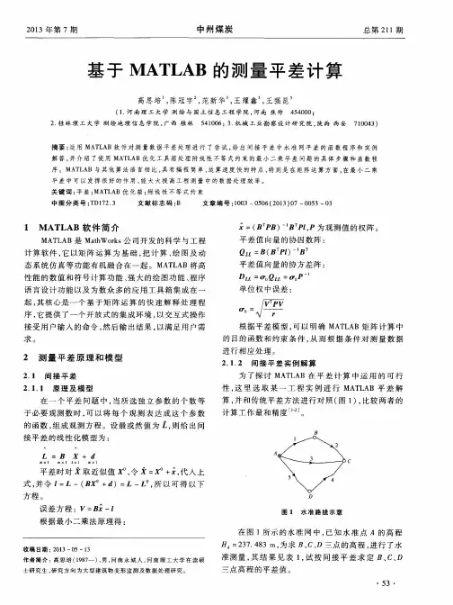
实验一一．设计原始资料水准网周密平差及精度评定示例。

如图所示水准网，有2个已知点，3个未知点，7个测段。

各已知数据及观测值见下表（1）已知点高程H1= H2=（2）高差观测值(m)高差观测值(m)端点高差观测值测段距离序号号1-3 11-4 22-3 32-4 43-4 53-5 65-2 7（3）求各待定点的高程；3-4点的高差中误差；3号点、4号点的高程中误差。

（提示，本网可采用以测段的高差为平差元素，采用间接平差法编写程序计算。

）二、水准网间接平差思路⑴．按照网型肯定已知水准点数H1 H2，未知水准点数u ，总点数n ，必要观测数t ，多余观测数r 。

⑵.肯定参数。

为平差后能直接求得待定点高程平差值，以3个待定点高程平差值为参数。

设3,4,5点的高程平差值别离为，， 。

⑶．列立条件方程.左侧为观测值（系数为1），右边为参数和常数项，并进一步改化成误差方程，最终写成矩阵形式。

取得系数矩阵A 和常数项L⑷.列立法方程，并解求法方程。

⑸．精度评定。

计算单位权中误差的估值：评定各待定点的高程中误差： 各待定点的精度即为： 评定高程平差值的精度： 四、平差程序设计思路1、 已知数据的输入需要输入的数据包括水准网中已知点数、未知点数和这些点的点号、已知高程和高差观测值、距离观测值等。

本程序采用文件方式进行输入，文件输入的格式如下： 第一行：已知点个数、未知点个数、观测值个数 第二行：点号 （已知点在前，为支点在后） 第三行：已知高程 （顺序与上一行的点号对应）第四行起：高差观测值，依照“起点点号，终点点号，高差观测值，距离观测值”的顺序输入。

2、 平差计算进程 （1）近似高程计算。

uc PV V r PV V T T -==20ˆσ120ˆˆ20ˆˆˆˆ-==bbx x x x N Q D σσjj X X j X Q ˆˆ0ˆˆσσ±=FN F F Q F Q BB T X X T h h 1ˆˆˆˆ-==X F hT ˆˆ=（2）列立观测值的误差方程。

[4] 武汉大学测绘学院 测量平 差学科 组. 误 差理论 与测 量 平差基础[ M] . 武汉: 武汉大学出版社, 2003.
[5] 姚德新. 土木工 程测量 学教程 [ M] . 北京: 中国 铁道 出 版社, 2003.
Adjustment Programming of Level Net on the Basis of MATLAB
Dxt
ln
式中: t 为未知点个数.
p11 0 0 p22
ss 00
,0
, w
0 s
.
, pnn
由于方程个数 小于未知量个数, 因此式( 3) 有 无群解, 取[ vv] 最小的一组解为最或然解[ 4] . 即
X = - ( BT PB )- BT Pl
( 4)
由此, 只要确定了系数阵 B, 权阵 P 和常数阵 l, 就
文章编号: 100124373( 2009) 0320029203
Vol. 28 No. 3 June 2009
基于 MAT LAB 的水准网平差程序设计*
李 建章
( 兰州交通大学 土木工程学院, 甘肃 兰州 730070)
摘 要: 设计了水准网数据结构, 并根据该数据结构将水准网边和点的相对位置关 系以及观测 数据、已知数据存 储
1 水准网数据结构设计
如图 1 所示, 水准网是由边和点两种要素构成 的, 其中每条边包含一个起点和一个终点, 且边具有 方向性, 其高差值为终点高程减去起点高程. 本文设 计了 ptT ab 和 lineT ab 两个表来存储水准网边点连 接关系以及观测数据和已知数据.
pt T ab 表用来存储所有的已知点和未知点. 程 序运行前用户需填写所有点的点号、已知点高程值 和已知点标志, 其余由程序自动完成. lineTab 则存 储每条观测边的首尾点号、观测高差以及线路长.