Mathematica简易教程

mathematica解方程
Mathematica是一款强大的数学软件，可以使用其内置的求解方程的功能来解决方程问题。

下面是使用Mathematica求解方程的一般步骤：
1. 输入方程：在Mathematica的Notebook界面中，输入要解决的方程，使用等号“=”表示方程的左右两侧。

2. 使用Solve函数求解：使用Solve函数，输入方程，指定要解的变量，运行程序即可求解方程。

例如：
Solve[x^2 - 2x + 1 == 0, x]
这个命令可以求解方程x^2 - 2x + 1 = 0，并返回方程的解。

3. 使用Reduce函数求解：如果方程的解比较复杂或者有多个解，可以使用Reduce函数。

Reduce函数可以找到方程的所有解，并给出条件。

例如：
Reduce[x^3 + 3x^2 + 3x + 1 == 0, x]
这个命令可以求解方程x^3 + 3x^2 + 3x + 1 = 0，并返回方程的所有解。

4. 使用NSolve函数求解数值解：如果方程无法用解析式表示，或者需要求解数值解，可以使用NSolve函数。

例如：
NSolve[x^2 - 2x + 1 == 0, x]
这个命令可以求解方程x^2 - 2x + 1 = 0 的数值解。

M athematica是美国Wolfram研究公司生产的一种数学分析型的软件，以符号计算见长，也具有高精度的数值计算功能和强大的图形功能。

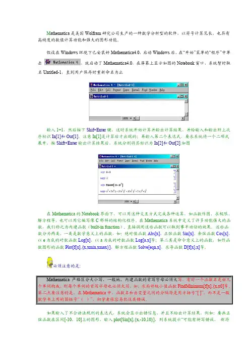
假设在Windows环境下已安装好Mathematica4.0，启动Windows后，在“开始”菜单的“程序”中单击，就启动了Mathematica4.0，在屏幕上显示如图的Notebook窗口，系统暂时取名Untitled-1，直到用户保存时重新命名为止输入1+1，然后按下Shif+Enter键，这时系统开始计算并输出计算结果，并给输入和输出附上次序标识In[1]和Out[1]，注意In[1]是计算后才出现的；再输入第二个表达式，要求系统将一个二项式展开，按Shift+Enter输出计算结果后，系统分别将其标识为In[2]和Out[2].如图在Mathematica的Notebook界面下，可以用这种交互方式完成各种运算，如函数作图，求极限、解方程等，也可以用它编写像C那样的结构化程序。

在Mathematica系统中定义了许多功能强大的函数，我们称之为内建函数（built-in function）, 直接调用这些函数可以取到事半功倍的效果。

这些函数分为两类，一类是数学意义上的函数，如：绝对值函数Abs[x]，正弦函数Sin[x]，余弦函数Cos[x]，以e为底的对数函数Log[x]，以a为底的对数函数Log[a,x]等；第二类是命令意义上的函数，如作函数图形的函数Plot[f[x],{x,xmin,xmax}]，解方程函数Solve[eqn,x]，求导函数D[f[x],x]等。

必须注意的是:Mathematica 严格区分大小写，一般地，内建函数的首写字母必须大写，有时一个函数名是由几个单词构成，则每个单词的首写字母也必须大写，如：求局部极小值函数FindMinimum[f[x],{x,x0]等。

第二点要注意的是，在Mathematica中，函数名和自变量之间的分隔符是用方括号“[ ]”，而不是一般数学书上用的圆括号“（）”，初学者很容易犯这类错误。

（整理）Mathematica入门教程.Mathematica入门教程Mathematica的基本语法特征如果你是第一次使用Mathematica，那么以下几点请你一定牢牢记住：Mathematica中大写小写是有区别的，如Name、name、NAME等是不同的变量名或函数名。

系统所提供的功能大部分以系统函数的形式给出，内部函数一般写全称，而且一定是以大写英文字母开头，如Sin[x],Conjugate[z]等。

乘法即可以用*，又可以用空格表示，如2 3＝2*3＝6 ,x y,2 Sin[x]等；乘幂可以用“^”表示，如x^0.5,T an[x]^y。

自定义的变量可以取几乎任意的名称，长度不限，但不可以数字开头。

当你赋予变量任何一个值，除非你明显地改变该值或使用Clear[变量名]或“变量名=.”取消该值为止，它将始终保持原值不变。

一定要注意四种括号的用法：()圆括号表示项的结合顺序，如(x+(y^x+1/(2x)));[]方括号表示函数，如Log[x],BesselJ[x,1]；{}大括号表示一个“表”(一组数字、任意表达式、函数等的集合)，如{2x,Sin[12Pi],{1+A,y*x}}；[[]]双方括号表示“表”或“表达式”的下标，如a[[2,3]]、{1,2,3}[[1]]=1。

Mathematica的语句书写十分方便，一个语句可以分为多行写，同一行可以写多个语句（但要以分号间隔）。

当语句以分号结束时，语句计算后不做输出（输出语句除外），否则将输出计算的结果。

一.数的表示及计算1.在Mathematica中你不必考虑数的精确度，因为除非你指定输出精度，Mathematica总会以绝对精确的形式输出结果。

例如：你输入In[1]:=378/123，系统会输出Out[1]:=126/41，如果想得到近似解，则应输入In[2]:=N[378/123,5],即求其5位有效数字的数值解，系统会输出Out[2]:=3.0732，另外Mathematica还可以根据你前面使用的数字的精度自动地设定精度。

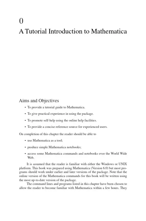
A Tutorial Introduction to MathematicaAims and Objectives•To provide a tutorial guide to Mathematica.•To give practical experience in using the package.•To promote self-help using the online help facilities.•To provide a concise reference source for experienced users.On completion of this chapter the reader should be able to•use Mathematica as a tool;•produce simple Mathematica notebooks;•access some Mathematica commands and notebooks over the World Wide Web.It is assumed that the reader is familiar with either the Windows or UNIX platform.This book was prepared using Mathematica(Version6.0)but most pro-grams should work under earlier and later versions of the package.Note that the online version of the Mathematica commands for this book will be written using the most up-to-date version of the package.The command lines and programs listed in this chapter have been chosen to allow the reader to become familiar with Mathematica within a few hours.They20.A Tutorial Introduction to Mathematicaprovide a concise summary of the type of commands that will be used throughout the text.New users should be able to start on their own problems after completing the chapter,and experienced users shouldfind this chapter an excellent source of reference.Of course,there are many Mathematica textbooks on the market for those who require further applications or more detail.If you experience any problems there are several options for you to take. There is an excellent index within Mathematica,and Mathematica commands, notebooks,programs,and output can also be viewed in color over the Web at Mathematica’s Information Center:/infocenter/Books/AppliedMathematics/The notebookfiles can be found at the links Calculus Analysis and Dynamical Systems.Download the zipped notebookfiles and Extract the relevantfiles from the archive onto your computer.0.1A Quick Tour of MathematicaTo start Mathematica,simply double-click on the Mathematica icon.In the UNIX environment,one types mathematica as a shell command.The author has used the Windows platform in the preparation of this material.When Mathematica starts up,a blank notebook appears on the computer screen entitled Untitled-1and some palettes with buttons may appear alongside.Some examples of palettes are given in Figure0.1.The buttons on the palettes serve essentially as additional keys on the user keyboard.Input to the Mathematica notebook can either be performed by typing in text commands or pointing and clicking on the symbols provided by various palettes and subpalettes.As many of the Mathematica programs in subsequent chapters of this book are necessarily text based,the author has decided to present the material using commands in their text format.However,the use of palettes can save some time in typing,and the reader may wish to experiment with the“clicking on palettes’’approach.Mathematica even allows users to create their own palettes;again readers mightfind this useful.Mathematica notebooks can be used to generate full publication-quality doc-uments.In fact,all of the Mathematica help pages have been created with interac-tive notebooks.The Help menu also includes an online version of the Mathematica book[1].The author recommends a brief tour of some of the help pages to give the reader an idea of how the notebooks can be used.For example,click on the Help toolbar at the top of the Mathematica graphical user interface and scroll down to Help browser....Simply type in Solve and ENTER.An interactive Mathemat-ica notebook will be opened showing the syntax,some related commands,and examples of the Solve command.The interactive notebooks from each chapter of this book can be downloaded from Mathematica’s Information Center:/infocenter/Books/AppliedMathematics/0.1.A Quick Tour of Mathematica3(a)(b)(c)(d)Figure0.1:Some Mathematica palettes:(a)Basic input palette.(b)Technical symbols,shapes,and icons.(c)Relational operators.(d)Relational arrows.The author has provided the reader with a tutorial introduction to Mathematica in Sections0.2,0.3,and0.4.Each tutorial should take no more than one hour to complete.The author highly recommends that new users go through these tutorials line by line;however,readers already familiar with the package will probably use Chapter0as reference material only.Tutorial One provides a basic introduction to the Mathematica package. Thefirst command line shows the reader how to input comments,which are extremely useful when writing long or complicated programs.The reader will type in(*This is a comment*)and then type SHIFT-ENTER or SHIFT-RETURN (hold down the SHIFT key and press ENTER).Mathematica will label thefirst input with In[1]:=(*This is a comment*).Note that no output is given for a comment.The second input line is simple arithmetic.The reader types 2+3-36/2+2ˆ3,and types SHIFT-ENTER to compute the result.Mathematica labels the second input with In[2]:=2+3-36/2+2ˆ3,and labels the corre-sponding output Out[2]=-5.As the reader continues to input new command40.A Tutorial Introduction to Mathematicalines,the input and output numbers change accordingly.This allows users to easily label input and output that may be useful later in the notebook.Note that all of the built-in Mathematica functions begin with capital letters and that the arguments are always enclosed in square brackets.Tutorial Two contains graphic commands and commands used to solve simple differential equations.Tutorial Three pro-vides a simple introduction to the Manipulate command and programming with Mathematica.The tutorials are intended to give the reader a concise and efficient intro-duction to the Mathematica package.Many more commands are listed in other chapters of the book,where the output has been included.Of course,there are many Mathematica textbooks on the market for those who require further appli-cations or more detail.A list of textbooks is given in the reference section of this chapter.0.2Tutorial One:The Basics(One Hour)There is no need to copy the comments,they are there to help you.Click on the Mathematica icon and copy the commands.Hold down the SHIFT key and press ENTER at the end of a line to see the answer or use a semicolon to suppress the output.You can interrupt a calculation at any time by typing ALT-COMMA or COMMAND-COMMA.A working Mathematica notebook of Tutorial One can be downloaded from the Mathematica Information Center,as indicated at the start of the chapter.Mathematica Command Lines CommentsIn[1]:=(*This is a comment*)(*Helps when writingprograms.*)In[2]:=2+3-36/2+2ˆ3(*Simple arithmetic.*)In[3]:=23*7(*Use space or*tomultiply.*)In[4]:=2/3+4/5(*Fraction arithmetic.*)In[5]:=2/3+4/5//N(*Approximate decimal.*)In[6]:=Sqrt[16](*Square root.*)In[7]:=Sin[Pi](*Trigonometric function.*) In[8]:=z1=1+2I;z2=3-4*I;z3=z1-z2/z1(*Complex arithmetic.*)In[9]:=ComplexExpand[Exp[z1]](*Express in form x+iy.*)In[10]:=Factor[xˆ3-yˆ3](*Factorize.*)In[11]:=Expand[%](*Expand the last resultgenerated.*)In[12]:=f=mu x(1-x)/.{mu->4,x->0.2}(*Evaluate f when mu=4andx=0.2.*)In[13]:=Clear[mu,x](*Clear values.*)0.2.Tutorial One:The Basics(One Hour)5In[14]:=Simplify[(xˆ3-yˆ3)/(x-y)](*Simplify an expression.*) In[15]:=Dt[xˆ2-3x+6,x](*Total differentiation.*)In[16]:=D[xˆ3yˆ5,{x,2},{y,3}](*Partial differentiation.*) In[17]:=Integrate[Sin[x]Cos[x],x](*Indefinite integration.*) In[18]:=Integrate[Exp[-xˆ2],{x,0,Infinity}](*Definite integration.*)In[19]:=Sum[1/nˆ2,{n,1,Infinity}](*An infinite sum.*)In[20]:=Solve[xˆ2-5x+6==0,x](*Solving equations.Rootsare in a list.*)In[21]:=Solve[xˆ2-5x+8==0,x](*A quadratic with complexroots.*)In[22]:=Abs[x]/.Out[21](*Find the modulus of theroots(see Out[21]).*)In[23]:=Solve[{xˆ2+yˆ2==1,x+3y==0}](*Solving simultaneousequations.*)In[24]:=Series[Exp[x],{x,0,5}](*Taylor series expansion.*) In[25]:=Limit[x/Sin[x],x->0](*Limits.*)In[26]:=f=Function[x,4x(1-x)](*Define a function.*)In[27]:=f[0.2](*Evaluate f(0.2).*)In[28]:=fofof=Nest[f,x,3](*Calculates f(f(f(x))).*)In[29]:=fnest=NestList[f,x,4](*Generates a list ofcomposite functions.*)In[30]:=fofofof=fnest[[4]](*Extract the4th elementof the list.*)In[31]:=u=Table[2i-1,{i,5}](*List the first5oddnatural numbers.*)In[32]:=%ˆ2(*Square the elements ofthe last result generated.*) In[33]:=a={2,3,4};b={5,6,7};(*Two vectors.*)In[34]:=3a(*Scalar multiplication.*)In[35]:=a.b(*Dot product.*)In[36]:=Cross[a,b](*Cross product.*)In[37]:=Norm[a](*Norm of a vector.*)In[38]:=A={{1,2},{3,4}};B={{5,6},{7,8}};(*Two matrices.*)In[39]:=A.B-B.A(*Matrix arithmetic.*)In[40]:=MatrixPower[A,3](*Powers of a matrix.*)In[41]:=Inverse[A](*The inverse of a matrix.*) In[42]:=Det[B](*The determinant of amatrix.*)60.A Tutorial Introduction to MathematicaIn[43]:=Tr[B](*The trace of a matrix.*) In[44]:=M={{1,2,3},{4,5,6},{7,8,9}}(*A matrix.*)In[45]:=Eigenvalues[M](*The eigenvalues of amatrix.*)In[46]:=Eigenvectors[M](*The eigenvectors of amatrix.*)In[47]:=LaplaceTransform[tˆ3,t,s](*Laplace transform.*)In[48]:=InverseLaplaceTransform[6/sˆ4,s,t](*Inverse Laplacetransform.*)In[49]:=FourierTransform[tˆ4Exp[-tˆ2],t,w](*Fourier transform.*)In[50]:=InverseFourierTransform[%,w,t](*Inverse Fouriertransform.*)In[51]:=Quit[](*Terminates Mathematicakernel session.*)0.3Tutorial Two:Plots and Differential Equations(One Hour)Mathematica has excellent graphical capabilities and many solutions of nonlinear systems are best portrayed graphically.The graphs produced from the input text commands listed below may be found in the Tutorial Two Notebook which can be downloaded from the Mathematica Information Center.Plots in other chapters of the book are referred to in many of the Mathematica programs at the end of each chapter.(*Plotting graphs.*)(*Set up the domain and plot a simple function.*)In[1]:=Plot[Sin[x],{x,-Pi,Pi}](*Plot two curves on one graph.*)In[2]:=Plot[{Cos[x],Exp[-.1x]Cos[x]},{x,0,60}](*Plotting with labels.*)In[3]:=Plot[Exp[-.1t]Sin[t],{t,0,60},AxesLabel->{"t","Current"},PlotRange->{-1,1}](*Contour plot with shading.*)In[4]:=ContourPlot[yˆ2/2-xˆ2/2+xˆ4/4,{x,-2,2},{y,-2,2}](*Contour plot with no shading.*)In[5]:=ContourPlot[yˆ2/2-xˆ2/2+xˆ4/4,{x,-2,2},{y,-2,2},0.3.Tutorial Two:Plots and Differential Equations(One Hour)7ContourShading->False](*Contour plot with20contours.*)In[6]:=ContourPlot[yˆ2/2-xˆ2/2+xˆ4/4,{x,-2,2},{y,-2,2}, Contours->20](*Surface plot.*)In[7]:=Plot3D[yˆ2/2-xˆ2/2+xˆ4/4,{x,-2,2},{y,-2,2}](*A parametric plot.*)In[8]:=ParametricPlot[{tˆ3-4t,tˆ2},{t,-3,3}](*3-D parametric curve.*)In[9]:=ParametricPlot3D[{Sin[t],Cos[t],t/3},{t,-10,10}](*Load the package and plot an implicit curve.*)In[10]:=<<Graphics‘ImplicitPlot‘In[11]:=ImplicitPlot[2xˆ2+3yˆ2==12,{x,-3,3},{y,-3,3}](*Solve a simple separable differential equation.*)In[12]:=DSolve[x’(t)==-x[t]/t,x[t],t](*Solve an initial value problem(IVP).*)In[13]:=DSolve[{x’(t)==-t/x[t],x[0]==1},x[t],t](*Solve a second-order ordinary differential equation (ODE).*)In[14]:=DSolve[{x’’[t]+5x’[t]+6x[t]==10Sin[t],x[0]==0, x’[0]==0},x[t],t](*Solve a system of two ODEs.*)In[15]:=DSolve[{x’[t]==3x[t]+4y[t],y’[t]==-4x[t]+3y[t]}, {x[t],y[t]},t](*Solve a system of three ODEs.*)In[16]:=DSolve[{x’[t]==x[t],y’[t]==y[t],z’[t]==-z[t]}, {x[t],y[t],z[t]},t](*Solve an IVP using numerical methods and plot a solution curve.*)In[17]:=u=NDSolve[{x’[t]==x[t](.1-.01x[t]),x[0]==50}, x,{t,0,100}]In[18]:=Plot[Evaluate[x[t]/.u],{t,0,100},PlotRange->All](*Plot a phase plane portrait.*)In[19]:=v=NDSolve[{x’[t]==.1x[t]+y[t],y’[t]==-x[t]+.1y[t], x[0]==.01,y[0]==0},{x[t],y[t]},{t,0,50}]80.A Tutorial Introduction to MathematicaIn[20]:=ParamericPlot[{x[t],y[t]}/.v,{t,0,50},PlotRange->All,PlotPoints->1000](*Plot a three-dimensional phase portrait.*)In[21]:=w=NDSolve[{x’[t]==z[t]-x[t],y’[t]==-y[t],z’[t] ==z[t]-17x[t]+16,x[0]==.8,y[0]==.8,z[0]==.8},{x[t],y[t],z[t]},{t,0,20}]In[22]:=ParametricPlot3D[Evaluate[{x[t],y[t],z[t]}/.w], {t,0,20},PlotPoints->1000,PlotRange->All](*A stiff van der Pol system of ODEs.*)In[23]:=Needs["DifferentialEquations‘InterpolatingFunctionAnatomy‘"];In[24]:=vanderpol=NDSolve[{Derivative[1][x][t]==y[t],Derivative[1][y][t]==1000*(1-x[t]ˆ2)*y[t]-x[t],x[0]==2,y[0]==0},{x,y},{t,5000}];In[25]:=T=First[InterpolatingFunctionCoordinates[First[x/.vanderpol]]];In[26]:=ListPlot[Transpose[{x[T],y[T]}/.First[vanderpol]], PlotRange->All]0.4The Manipulate Command and SimpleMathematica ProgramsSections0.1,0.2,and0.3illustrate the interactive nature of Mathematica.More involved tasks will require more code.Note that Mathematica is very different from procedural languages such as C,Pascal,or Fortran.An afternoon spent browsing through the pages listed at the Mathematica Information Center will convince readers of this fact.The Manipulate command is new in Version6.0and is very useful in the field of dynamical systems.Manipulate[expr,{u,u min,u max}]generates a version of expr with controls added to allow interactive manipulation of the value of u.The Manipulate CommandOn execution of the Manipulate command a parameter slider appears in the note-book.Solutions change as the slider is moved left and right.(*Example1:Solving simultaneous equations as the parameter a varies.See Exercise6in Chapter 3.*)In[1]:=Manipulate[Solve[{x(1-y-a x)==0,y(-1+x-a y)==0}], {a,0,1}](*Showing the solution lying wholly in the first quadrant.*) In[2]:=Manipulate[Plot[{1-a x,(x-1)/a},{x,0,2}],{a,0.01,1}]0.4.The Manipulate Command and Simple Mathematica Programs 9(*Example 2:Evaluating functions of functions to the fifth iteration.*)In[3]:=f=Function[x,4x (1-x)];In[4]:=Manipulate[Expand[Nest[f,x,d]],{d,1,5,1}](*Stepsof 1.*)(*Example 3:Solving a differential equation as twoparameters vary.In this case,the damping and restoring terms when modeling a simple pendulum.*)In[5]:=Manipulate[DSolve[{x’’[t]+b x’[t]+c x[t]==0,x[0]==1,x’[0]==0},x[t],t],{b,0,2},{c,0,5}](*The solution curves.*)In[6]:=Manipulate[soln=NDSolve[{x’’[t]+b x’[t]+c x[t]==0,x[0]==1,x’[0]==0},x[t],{t,0,100}];Plot[Evaluate[x[t]/.soln],{t,0,100},PlotRange->All],{b,0,5},{c,0,5}]Many Manipulate demonstrations are available from the Wolfram Demon-strations Project:/Simple Mathematica ProgramsEach Mathematica program is displayed between horizontal lines and kept short to aid in understanding;the output is also included.Modules and local variables.Aglobal variable t is unaffected by the local variable t used in a module.In[1]:=Norm3d[a_,b_,c_]=Module[{t},t=Sqrt[aˆ2+bˆ2+cˆ2]]Out [1]= a 2+b 2+c 2In[2]:=Norm3d[3,4,5]Out [2]=5√2The Do command.The first ten terms of the Fibonacci sequence.In[3]:=F[1]=1;F[2]=1;Nmax=10;In[4]:=Do[F[i]=F[i-1]+F[i-2],{i,3,Nmax}]In[5]:=Table[F[i],{i,1,Nmax}]Out [5]={1,1,2,3,5,8,13,21,34,55}100.A Tutorial Introduction to MathematicaIf,then,else construct.In[6]:=Num=1000;If[Num>0,Print["Num is positive"],If[Num==0, Print["Num is zero"],Print["Num is negative"]]]Out[6]=Num is positiveConditional statements with more than two alternatives.In[7]:=r[x_]=Switch[Mod[x,3],0,a,1,b,2,c]Out[7]=Switch[Mod[x,3],0,a,1,b,2,c]In[8]:=r[7]Out[8]=bWhich.Defining the tent function.In[9]:=T[x_]=Which[0<=x<1/2,mu x,1/2<=x<=1,mu(1-x)]Out[9]=Which[0≤x<1/2,mu x,1/2≤x≤1,mu(1−x)]In[10]:=T[4/5]Out[10]=mu5For pute f(x),f(f(x)),and f(f(f(x))).In[11]:=For[i=1;t=x,i<4,i++,t=mu t(1-t);Print[Factor[t]]] Out[11]=−mu(−1+x)x−mu2(−1+x)x(1−mu x+mu x2)−mu3(−1+x)x(1−mu x+mu x2)(1−mu2x+mu2x2+mu3x2−2mu3x3+mu3x4)Plotting solution curves.Solutions to the pendulum problem.See Figure0.2. In[12]:=ode1[x0_,y0_]:=NDSolve[{x’[t]==y[t],y’[t]==-25x[t], x[0]==x0,y[0]==y0},{x[t],y[t]},{t,0,6}];In[13]:=sol1[1]=ode1[1,0];In[14]:=ode2[x0_,y0_]:=NDSolve[{x’[t]==y[t],y’[t]==-2y[t]-25x[t],x[0]==x0,y[0]==y0},{x[t],y[t]},{t,0,6}];In[15]:=sol2[1]=ode2[1,0];In[16]:=p1=Plot[Evaluate[Table[{x[t]}/.sol1[i],{i,1}]], {t,0,6},PlotRange->All,PlotPoints->100,PlotStyle->Dashing[{.02}]];0.5.Hints for Programming 11123456t10.50.51xFigure 0.2:Harmonic and damped motion of a pendulum.In[17]:=p2=Plot[Evaluate[Table[{x[t]}/.sol2[i],{i,1}]],{t,0,6},PlotRange->All,PlotPoints->100];In[18]:=Show[{p1,p2},PlotRange->All,AxesLabel->{"t","x"},Axes->True,TextStyle->{FontSize->15}]0.5Hints for ProgrammingThe Mathematica language contains very powerful commands,which means that some complex programs may contain only a few lines of code.Of course,the only way to learn programming is to sit down and try it yourself.This section has been included to point out common errors and give advice on how to troubleshoot.Remember to check the help and index pages in Mathematica and the Web if the following does not help you with your particular problem.Common typing errors.The author strongly advises new users to type Tutorials One,Two,and Three into their own notebooks.This should reduce typing errors.•Type SHIFT-ENTER at the end of every command line.•If a command line is ended with a semicolon,the output will not be displayed.•Make sure brackets,parentheses,etc.,match up in correct pairs.•Remember that all of the built-in Mathematica functions begin with capital letters and that the arguments are always enclosed in square brackets.•Remember Mathematica is case sensitive.•Check the syntax;type ?Solve to list syntax for the Solve command,for example.120.A Tutorial Introduction to MathematicaProgramming tips.The reader should use the Mathematica programs listed in Section 0.4to practice simple programming techniques.•It is best to clear values at the start of a large program.•Use comments throughout a program.You will find them extremely useful in the future.•Use Modules or Blocks to localize variables.This is especially useful for very large programs.•If a program involves a large number of iterations,for example,50,000,then run it for three iterations first and list all output.•If the computer is not responding hold ALT-COMMA or COMMAND-COMMA and try reducing the size of the problem.•Read the error message printed by Mathematica and click on More…if necessary.•Find a similar Mathematica program in a book or on the Web,and edit it to meet your needs.•Check which version of Mathematica you are using.The syntax of some commands may have altered.0.6Mathematica Exercises1.Evaluate the following:(a)4+5−6;(b)312;(c)sin (0.1π);(d)(2−(3−4(3+7(1−(2(3−5))))));(e)25−34×23.2.Given thatA =⎛⎝12−10103−12⎞⎠,B =⎛⎝123112012⎞⎠,C =⎛⎝21101−1422⎞⎠,determine the following:(a)A +4BC ;(b)the inverse of each matrix if it exists;0.6.Mathematica Exercises 13(c)A 3;(d)the determinant of C ;(e)the eigenvalues and eigenvectors of B .3.Given that z 1=1+i ,z 2=−2+i ,and z 3=−i ,evaluate the following:(a)z 1+z 2−z 3;(b)z 1z 2z 3;(c)e z 1;(d)ln (z 1);(e)sin (z 3).4.Evaluate the following limits if they exist:(a)lim x →0sin x x ;(b)lim x →∞x 3+3x 2−52x 3−7x;(c)lim x →πcos x +1x −π;(d)lim x →0+1x;(e)lim x →02sinh x −2sin xcosh x −1.5.Find the derivatives of the following functions:(a)y =3x 3+2x 2−5;(b)y =√1+x 4;(c)y =e x sin x cos x ;(d)y =tanh x ;(e)y =x ln x .6.Evaluate the following definite integrals:(a) 1x =03x 3+2x 2−5dx ;(b) ∞x =11x 2dx ;(c) ∞−∞e −x 2dx ;(d) 101√xdx ;(e)2πsin (1/t)t 2dt .7.Graph the following:140.A Tutorial Introduction to Mathematica(a)y=3x3+2x2−5;(b)y=e−x2,for−5≤x≤5;(c)x2−2xy−y2=1;(d)z=4x2e y−2x4−e4y for−3≤x≤3and−1≤y≤1;(e)x=t2−3t,y=t3−9t for−4≤t≤4.8.Solve the following differential equations:(a)dydx =x2y,given that y(1)=1;(b)dydx =−yx,given that y(2)=3;(c)dydx =x2y3,given that y(0)=1;(d)d2xdt2+5dxdt+6x=0,given that x(0)=1and˙x(0)=0;(e)d2xdt2+5dxdt+6x=sin(t),given that x(0)=1and˙x(0)=0.9.Carry out100iterations on the recurrence relationx n+1=4x n(1−x n),given that(a)x0=0.2and(b)x0=0.2001.List thefinal10iterates in each case.10.Type?While to read the help page on the While e a whileloop to program Euclid’s algorithm forfinding the greatest common divisor of two e your program tofind the greatest common divisor of 12,348and14,238.Recommended Textbooks[1]S.Wolfram,The Mathematica Book,6th ed.(electronic),Wolfram Media,Champaign,IL,2007;included with Mathematica®Version6.0.[2]D.McMahon and D.M.Topa,A Beginner’s Guide to Mathematica,Chapmanand Hall,London,CA,2006.[3]G.Baumann,Mathematica for Theoretical Physics:Classical Mechanicsand Nonlinear Dynamics,Springer-Verlag,New York,2005.[4]G.Baumann,Mathematica for Theoretical Physics:Electrodynamics,Quan-tum Mechanics,General Relativity,and Fractals,Springer-Verlag,New York,2005.[5]M.Trott,The Mathematica Guidebook for Numerics,Springer-Verlag,NewYork,2005.Recommended Textbooks15 [6]M.Trott,The Mathematica Guidebook for Symbolics,Springer-Verlag,NewYork,2005.[7]M.Trott,The Mathematica Guidebook:Graphics,Springer-Verlag,NewYork,2004.[8]M.Trott,The Mathematica Guidebook:Programming,Springer-Verlag,New York,2004.[9]E.Don,Schaum’s Outline of Mathematica,McGraw–Hill,New York,2000.。

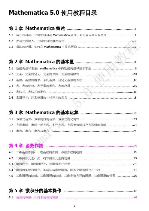
Mathematica 5.0使用教程目录第1章Mathematica概述 (3)1.1 运行和启动：介绍如何启动Mathematica软件，如何输入并运行命令 (3)1.2 表达式的输入：介绍如何使用表达式 (5)1.3 帮助的使用：如何在mathematica中寻求帮助 (6)第2章Mathematica的基本量 (8)2.1 数据类型和常量：mathematica中的数据类型和基本常量 (8)2.2 变量：变量的定义、变量的替换、变量的清除等 (10)2.3 函数：函数的概念，系统函数，自定义函数的方法 (12)2.4 表：表的创建，表元素的操作，表的应用 (15)2.5 表达式：表达式的操作 (16)2.6 常用符号：经常使用的一些符号的意义 (19)第3章Mathematica的基本运算 (19)3.1 多项式运算：多项的四则运算，多项式的化简等 (19)3.2 方程求解：求解一般方程，条件方程，方程数值解以及方程组的求解 (21)3.3 求积、求和：求积与求和 (24)第4章函数作图 (25)4.1 二维函数作图：一般函数的作图，参数方程的绘图 (25)4.2 二维图形元素：点、线等图形元素的使用 (29)4.3 图形样式：图形的样式，对图形进行设置 (31)4.4 图形的重绘和组合：重新显示所绘图形，将多个图形组合在一起 (33)4.5 三维图形的绘制：三维图形的绘制，三维参数方程的图形，三维图形的设置 (36)第5章微积分的基本操作 (42)5.1 函数的极限：如何求函数的极限 (42)5.2 导数与微分：如何求函数的导数、微分 (43)5.3 定积分与不定积分：如何求函数的不定积分和定积分，以及数值积分 (45)5.4 多变量函数的微分：如何求多元函数的偏导数、微分 (47)5.5 多变量函数的积分：如何计算重积分 (49)第6章微分方程的求解 (51)6.1 微分方程的解：微分方程的求解 (51)6.2 微分方程的数值解：如何求微分方程的数值解 (53)第7章Mathematica程序设计 (54)7.1 模块：模块的概念和定义方法 (54)7.2 条件结构：条件结构的使用和定义方法 (56)7.3 循环结构：循环结构的使用 (59)7.4 流程控制 (61)第8章Mathematica中的常用函数 (63)8.1 运算符和一些特殊符号：常用的和不常用一些运算符号 (63)8.2 系统常数：系统定义的一些常量及其意义 (63)8.3 代数运算：表达式相关的一些运算函数 (64)8.4 解方程：和方程求解有关的一些操作 (65)8.5 微积分相关函数：关于求导、积分、泰勒展开等相关的函数 (65)8.6 多项式函数：多项式的相关函数 (66)8.7 随机函数：能产生随机数的函数函数 (67)8.8 数值函数：和数值处理相关的函数，包括一些常用的数值算法 (67)8.9 表相关函数：创建表，表元素的操作，表的操作函数 (68)8.10 绘图函数：二维绘图，三维绘图，绘图设置，密度图，图元，着色，图形显示等函数 (69)8.11 流程控制函数 (72)第1章Mathematica概述1.1 Mathematica的启动和运行Mathematica是由美国物理学家Stephen Wolfram领导的一个小组开发进行量子力学研究的，软件开发成功促使Stephen Wolfram与1987年创建Wolfram研究公司，并推出了Mathematica1.0。

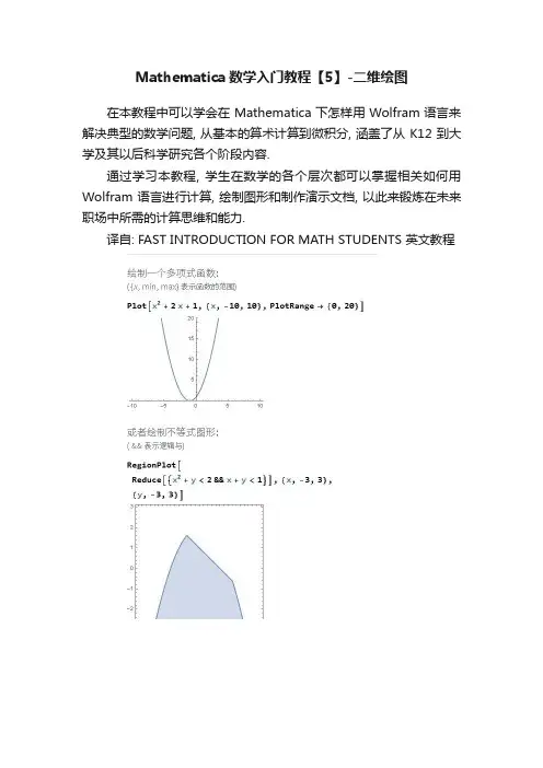
Mathematica数学入门教程【5】-二维绘图
在本教程中可以学会在 Mathematica 下怎样用 Wolfram 语言来解决典型的数学问题, 从基本的算术计算到微积分, 涵盖了从 K12 到大学及其以后科学研究各个阶段内容.
通过学习本教程, 学生在数学的各个层次都可以掌握相关如何用Wolfram 语言进行计算, 绘制图形和制作演示文档, 以此来锻炼在未来职场中所需的计算思维和能力.
译自: FAST INTRODUCTION FOR MATH STUDENTS 英文教程
好了, 现在让我们在下一篇的Mathematica 快速数学入门课堂再
见. 这里感谢各位每一位看到这里的老师和朋友!
Thank You, Everyone!
本入门教程全部内容:
1 - 指令的输入
2 - 分数与小数
3 - 变量和函数
4 - 代数
5 - 2D绘图
6 - 几何
7 - 三角学
8 - 极坐标
9 - 指数函数和对数
10 - 极限
11 - 微分
12 - 积分
13 - 序列
14 - 求和
15 - 级数
16 - 更多2D绘图
17 - 3D绘图
18 - 多元微积分
19 - 矢量分析和可视化
20 - 微分方程
21 - 复分析
22 - 矩阵和线性代数
23 - 离散数学
24 - 概率
25 - 统计
26 - 数据图和最佳拟合曲线
27 - 群论
28 - 数学智力题
29 - 互动模式
30 - 数学排版
31 - 笔记本文档
32 - 云部署。

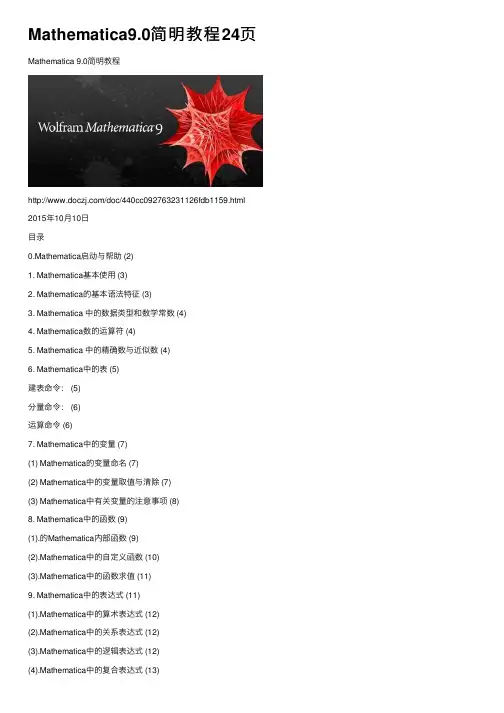
Mathematica9.0简明教程24页Mathematica 9.0简明教程/doc/440cc092763231126fdb1159.html 2015年10⽉10⽇⽬录0.Mathematica启动与帮助 (2)1. Mathematica基本使⽤ (3)2. Mathematica的基本语法特征 (3)3. Mathematica 中的数据类型和数学常数 (4)4. Mathematica数的运算符 (4)5. Mathematica 中的精确数与近似数 (4)6. Mathematica中的表 (5)建表命令： (5)分量命令： (6)运算命令 (6)7. Mathematica中的变量 (7)(1) Mathematica的变量命名 (7)(2) Mathematica中的变量取值与清除 (7)(3) Mathematica中有关变量的注意事项 (8)8. Mathematica中的函数 (9)(1).的Mathematica内部函数 (9)(2).Mathematica中的⾃定义函数 (10)(3).Mathematica中的函数求值 (11)9. Mathematica中的表达式 (11)(1).Mathematica中的算术表达式 (12)(2).Mathematica中的关系表达式 (12)(3).Mathematica中的逻辑表达式 (12)(4).Mathematica中的复合表达式 (13)10.Mathematica 中的⼀些符号和语句 (13)(1).Mathematica中的专⽤符 (13)(2).Mathematica中的屏幕输出语句 (14)11. 绘图 (15)（⼀）．Mathematica绘图命令有如下⼀些常⽤形式： (15)（⼆）．绘图命令中的选择项参数的形式为: (18)Mathematica⾃1988年由美国的Wolfram Research公司⾸次推出，是⼀个功能强⼤的常⽤数学软件, 不但可以解决数学中的数值计算问题, 还可以解决符号演算问题, 并且能够⽅便地绘出各种函数图形。

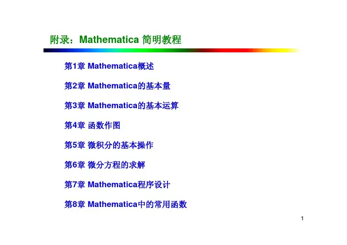
附录：Mathematica 简明教程第1章Mathematica概述第2章Mathematica的基本量第3章Mathematica的基本运算第4章函数作图第5章微积分的基本操作第6章微分方程的求解第7章Mathematica程序设计第8章Mathematica中的常用函数12第一章：Mathematica 概述在Windows环境下已安装好Mathematica4.0，启动Windows 后，在“开始”菜单的“程序”中单击，就启动了Mathematica4.0，在屏幕上显示如图的Notebook 窗口，系统暂时取名Untitled-1，直到用户保存时重新命名为止：输入1+1，然后按下Shift + Enter 键，这时系统开始计算并输出计算结果，并给输入和输出附上次序标识In[1]和Out[1]；再输入第二个表达式，要求系统将一个二项式展开，按Shift+Enter 输出计算结果后，系统分别将其标识为In[2]和Out[2]。

在Mathematica 的Notebook 界面下，可以用这种交互方式完成各种运算，如函数作图，求极限、解方程等，也可以用它编写像C 那样的结构化程序。

在Mathematica 系统中定义了许多功能强大的函数，可以直接调用这些函数。

这些函数分为两类，一类是常用数学函数；第二类是功能函数，如作函数图形的函数Plot[f[x],{x,xmin,xmax}]，解方程函数Solve[eqn,x]等。

1.1.1 Mathematica 的启动和运行第一章：Mathematica概述错误信息：如果输入了不合语法规则的表达式，系统会显示出错信息，并且不给出计算结果。

（1）Mathematica 区分字母的大小写；（2）所有指令的首字母大写；（3）括号的匹配。

例如：要画正弦函数在区间[-10，10]上的图形，输入plot[Sin[x],{x,-10,10}]，则系统提示“可能有拼写错误，新符号‘plot’很像已经存在的符号‘Plot’”，实际上，系统作图命令“Plot”第一个字母必须大写，一般地，系统内建函数首写字母都要大写。

Mathematica教程Mathematica5教程第1章Mathematica概述1.1 运⾏和启动：介绍如何启动Mathematica软件，如何输⼊并运⾏命令1.2 表达式的输⼊：介绍如何使⽤表达式1.3 帮助的使⽤：如何在mathematica中寻求帮助第2章Mathematica的基本量2.1 数据类型和常量：mathematica中的数据类型和基本常量2.2 变量：变量的定义，变量的替换，变量的清除等2.3 函数：函数的概念，系统函数，⾃定义函数的⽅法2.4 表：表的创建，表元素的操作，表的应⽤2.5 表达式：表达式的操作2.6 常⽤符号：经常使⽤的⼀些符号的意义第3章Mathematica的基本运算3.1 多项式运算：多项的四则运算，多项式的化简等3.2 ⽅程求解：求解⼀般⽅程，条件⽅程，⽅程数值解以及⽅程组的求解3.3 求积求和：求积与求和第4章函数作图4.1 ⼆维函数作图：⼀般函数的作图，参数⽅程的绘图4.2 ⼆维图形元素：点，线等图形元素的使⽤4.3 图形样式：图形的样式，对图形进⾏设置4.4 图形的重绘和组合：重新显⽰所绘图形，将多个图形组合在⼀起4.5 三维图形的绘制：三维图形的绘制，三维参数⽅程的图形，三维图形的设置第5章微积分的基本操作5.1 函数的极限：如何求函数的极限5.2 导数与微分：如何求函数的导数，微分5.3 定积分与不定积分：如何求函数的不定积分和定积分，以及数值积分5.4 多变量函数的微分：如何求多元函数的偏导数，微分5.5 多变量函数的积分：如何计算重积分5.6 幂级数：幂级数的展开及其计算第6章微分⽅程的求解6.1 微分⽅程的解：微分⽅程的求解6.2 微分⽅程的数值解：如何求微分⽅程的数值解第7章Mathematica程序设计7.1 模块：模块的概念和定义⽅法7.2 条件结构：条件结构的使⽤和定义⽅法7.3 循环结构：循环结构的使⽤7.4 流程控制：简单介绍控制函数第8章Mathematica中的常⽤函数8.1 运算符和⼀些特殊符号：常⽤的和不常⽤⼀些运算符号8.2 系统常数：系统定义的⼀些常量及其意义8.3 代数运算：表达式相关的⼀些运算函数8.4 解⽅程：和⽅程求解有关的⼀些操作8.5 微积分相关函数：关于求导，积分，泰勒展开等相关的函数8.6 多项式函数：多项式的相关函数8.7 随机函数：能产⽣随机数的函数函数8.8 数值函数：和数值处理相关的函数，包括⼀些常⽤的数值算法8.9 表相关函数：创建表，表元素的操作，表的操作函数8.10 绘图函数：⼆维绘图，三维绘图，绘图设置，密度图，图元，着⾊，图形显⽰等函数8.11 流程控制函数第1章Mathematica概述1.1 Mathematica的启动和运⾏Mathematica是美国Wolfram研究公司⽣产的⼀种数学分析型的软件，以符号计算见长，也具有⾼精度的数值计算功能和强⼤的图形功能。

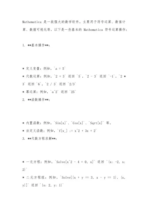
Mathematica是一款强大的数学软件，主要用于符号运算、数值计算、数据可视化等。

以下是一些基本的Mathematica符号运算操作：1. **基本操作**：* 定义变量：例如，`a = 5`* 代数运算：例如，`2 + 3` 返回 `5`，`2 - 3` 返回 `-1`，`2 * 3` 返回 `6`，`2 / 3` 返回 `2/3`* 幂运算：例如，`a^2` 返回 `25`2. **函数操作**：* 内置函数：例如，`Sin[x]`、`Cos[x]`、`Sqrt[x]` 等。

* 自定义函数：例如，`f[x_] := x^2 + 3x + 2`3. **代数方程求解**：* 一元方程：例如，`Solve[x^2 - 4 = 0, x]` 返回 `{x: -2, x: 2}`* 二元方程组：例如，`Solve[{x + y == 3, x - y == 1}, {x, y}]` 返回 `{x: 2, y: 1}`4. **微积分运算**：* 求导数：例如，`D[f[x], x]` 对于函数 `f[x] = x^2` 返回`2x`* 求积分：例如，`Integrate[f[x], x]` 对于函数 `f[x] = x^2` 返回 `x^3/3`5. **极限和连续性**：* 求极限：例如，`Limit[f[x], x -> a]` 对于函数 `f[x] = x^2` 当 `x -> a` 时返回 `a^2`（注意，这仅在 `a = -∞, +∞, 或 a 是某函数的可去间断点时才有意义）6. **级数和序列**：* 级数求和：例如，对于级数 `1 + 1/2 + 1/3 + ...`，使用`Sum[1/n, {n, 1, Infinity}]` 可得结果为`π^2/6`。

7. **符号表达式的简化**：* 化简表达式：例如，使用 `Simplify[expr]` 可以化简符号表达式。

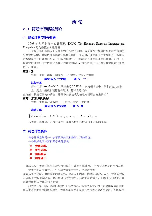
绪论0.1 符号计算系统简介# 数值计算与符号计算1946 年世界上第一台计算机ENIAC (The Electronic Numerical Integrator and Computer) 是为数值积分服务的。

一提起计算机求解人们立刻想到的是数值求解，这是因为计算机的早期应用范围主要是数值求解。

其实数值求解是计算机求解的一个方面，计算机进行计算的另一方面即对数学表示式的处理已形成一门新的科学分支，称为符号计算或计算机代数，它是一门研究使用计算机进行数学公式推导的理论和方法，演算数学公式的理论和算法是它研究的中心课题。

数值计算：常量、变量、函数、运算符--〉数值、字符、逻辑量表达式€一个值多€一近似计算例：计算y=sin10+ln10。

其结果是1.75856。

在高级语言中，算术表达式由常量、变量、函数和运算符等组成，算术表达式的值为某一精度范围内的数值。

计算各类表达式的值是高级语言的主要工作。

符号计算(计算机代数):常量、变量值、函数值--〉数值、字符、逻辑量表达式€表达式多€多准确计算x 2 sin xdx ＝-(-2 + x 2 )cos x + 2 x sin x与数值计算相比，符号计算对计算机硬件和软件提出了更高的要求。

# 符号计算系统符号计算系统是一个表示数学知识和数学工具的系统，一个集成化的计算机数学软件系统。

# 数值计算、# 符号计算、# 图形演示# 程序设计公式推导、数值计算和图形可视化操作一致性和连贯性。

符号计算系统的对象从初等数学到高等数学，几乎涉及所有数学学科。

包括各种数学表达式的化简、多项式的四则运算、求最大公因式、因式分解(factor)、常微分方程和偏微分方程的解函数。

各种特殊函数的推导、函数的级数展开、矩阵和行列式的各种运算和线性方程组的符号解等。

和数值计算一样，算法也是符号计算的核心。

就算法而言，符号计算比数值计算能继承更多的更丰富的数学遗产，古典数学家许多算法仍然是核心算法的成员，近代数学的算法成果也在不断地充实到符号计算中。

Mathematica入门教程第1篇第1章MATHEMATICA概述 (3)1.1 M ATHEMATICA的启动与运行 (3)1.2 表达式的输入 (4)1.3 M ATHEMATICA的联机帮助系统 (6)第2章MATHEMATICA的基本量 (8)2.1 数据类型和常数 (8)2.2 变量 (10)2.3 函数 (11)2.4 表 (14)2.5 表达式 (17)2.6 常用的符号 (19)2.7 练习题 (19)第2篇第3章微积分的基本操作 (20)3.1 极限 (20)3.2 微分 (20)3.3 计算积分 (22)3.4 无穷级数 (24)3.5 练习题 (24)第4章微分方程的求解 (26)4.1 微分方程解 (26)4.2 微分方程的数值解 (26)4.3 练习题 (27)第3篇第5章MATHEMATICA的基本运算 (28)5.1 多项式的表示形式 (28)5.2 方程及其根的表示 (29)5.3 求和与求积 (32)5.4 练习题 (33)第6章函数作图 (35)6.1 基本的二维图形 (35)6.2 二维图形元素 (40)6.3 基本三维图形 (42)6.4 练习题 (46)第4篇第7章MATHEMATICA函数大全 (48)7.1 运算符和一些特殊符号，系统常数 (48)7.2 代数计算 (49)7.3 解方程 (50)7.4 微积分 (50)7.5 多项式函数 (51)7.6 随机函数 (52)7.7 数值函数 (52)7.8 表相关函数 (53)7.9 绘图函数 (54)7.10 流程控制 (57)第8章MATHEMATICA程序设计 (59)8.1 模块和块中的变量 (59)8.2 条件结构 (61)8.3 循环结构 (63)8.4 流程控制 (65)8.5 练习题 (67)--------------习题与答案在68页-------------------第1章Mathematica概述1.1 Mathematica的启动与运行Mathematica是美国Wolfram研究公司生产的一种数学分析型的软件，以符号计算见长，也具有高精度的数值计算功能和强大的图形功能。