The Triggering and Bias of Radio Galaxies

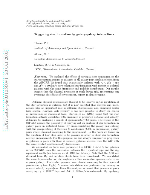
a rXiv:as tr o-ph/31560v12Oct23Recycling intergalactic and interstellar matter IAU Symposium Series,Vol.217,2004Pierre-Alain Duc,Jonathan Braine and Elias Brinks,eds.Triggering star formation by galaxy-galaxy interactions Tissera,P.B.Institute of Astronomy and Space Science,Conicet Alonso,plejo Astron´o mico El Leoncito,Conicet Lambas,D.G.&Coldwell,G.IATE,Observatorio Astron´o mico C´o rdoba.Conicet Abstract.We analyzed the effects of having a close companion on the star formation activity of galaxies in 8K galaxy pair catalog selected from the 2dFGRS.We found that,statistically,galaxies with r p <25h −1kpc and ∆V <100km /s have enhanced star formation with respect to isolated galaxies with the same luminosity and redshift distribution.Our results suggest that the physical processes at work during tidal interactions can overcome the effects of environment,expect in dense regions.Different physical processes are thought to be involved in the regulation of the star formation in galaxies,but it is now accepted that mergers and inter-actions play an important role as different observational and numerical works have shown.However,only recently it has been possible to study the effects of interactions on statistical basis.Barton et al.(2000)found that the star formation activity correlates with proximity in projected distance and velocity difference by analyzing a sample of approximately 200pairs.The release of the 2dFGRS opened the possibility of carrying out an analysis of star formation in galaxy pairs on statistical basis.By cross-correlating the galaxy pair catalog with the group catalog of Merch´a n &Zandivarez (2003,in preparation)galaxypairs where classified according to the environment.In this work we focuse on the question of how close have to be galaxies in order to show star formation activity enhancement.For this purpose,we will always compare the properties of galaxies in pairs with those of isolated galaxies selected from the 2dF with the same redshift and luminosity distribution.We estimated the birth rate parameter b =SF R/<SF R >for galaxies in the 2dFGRS from the correlation between the ηspectral type and the H αequivalent width (see Lambas et al.2003for details).Note that the SFR are deduced from H αand no dust effects have been considered.We calculated the mean b parameter for the neighbors within concentric spheres centered at a given galaxy.The center galaxies were chosen according to their spectral parameters η(see Fig1a)A similar calculation was performed by binning in relative velocity separation.From this analysis we found that galaxies in pairs satisfying r p <100h −1kpc and ∆V <350km /s is enhanced.By applying12Author &Coauthorthese two criteria,we selected approximately 9000pairs with z <0.1in high and low density environments.We also constructed a galaxy control sample by identifying galaxies with non close companion in the field (or cluster)with the same redshift and luminosity distribution as galaxies in pairs.We then estimated the mean b parameters for galaxies in pairs in projected and relative velocity bins,and the mean b value of the control sample.By equating them,we found that the star formation activity is statistically enhanced by the presence of a companion from r p ≈25h −1kpc and ∆V <100km /s in comparison to isolated galaxies (see Fig.1b).This analysis extended to galaxy pairs in groups (Alonso et al.2004)yields similar results,except for galaxy pairs in very high density regions where the both colors and b show no star formation activity in the present.Hence,statistically,tidal fields seem to be efficient in enhancing the star formation activity for very close pairs.The relative velocity and projected separation thresholds are independent of environment,suggesting that galaxy-galaxy interactions can be a main,ubiquitous motor of star formation activity in the Universe.00.20.40.60.811.21.41.6Figure 1.a)Mean birthrate parameter b as a function of relative projected separation r p of galaxies with η>3.5(solid line),η>−1.4(dotted line)and no ηrestriction (dotted-dashed line).The dotted vertical line depict the spatial separation threshold identification.b)Mean b parameters estimated in projected distance bins for galaxies in interacting pairs in the field.The small box shows the fraction f ⋆of galaxies with b >¯b .The dashed horizontal lines represent the mean b parameter for the corresponding control sample.ReferencesAlonso,M.S,Tissera,P.B.,Coldwell,G.,Lambas,D.G.,2003,submitted.Barton E.J.,Geller M.J.,Kenyon S.J.,2000,ApJ,530,660Lambas,D.G.,Tissera,P.B.,Alonso,M.S.Coldwell,G.2003,MNRAS inpress。

Host Galaxies and the Unification of Radio-Loud AGNC.M.Urry,R.Scarpa,M.O’Dowd,R.Falomo,M.Giavalisco,J.E.Pesce&A.TrevesABSTRACTOur HST WFPC2survey of109BL Lac objects,from six complete radio-,X-ray-, and optically-selected catalogs,probes the host galaxies of low-luminosity radio sources in the redshift range0<z<1.35.The host galaxies are luminous ellipticals,well matched in radio power and galaxy magnitude to FR I radio galaxies.Similarly,the host galaxies of high luminosity quasars occupy the same region of this plane as FR II radio galaxies (matched in redshift).This strongly supports the unification of radio-loud AGN,and suggests that studying blazars at high redshift is a proxy for investigating less luminous(to us)but intrinsically identical radio galaxies,which are harder tofind at high z.Accordingly, the difference between low-power jets in BL Lac objects and high-power jets in quasars can then be related to the FR I/FR II dichotomy;and the evolution of blazar host galaxies or their nuclei(jets)should correspond to the evolution of radio galaxies.Sample and ObservationsBL Lacertae objects(BL Lacs)are AGN of the blazar class—highly luminous, polarized and variable AGN.Unified Schemes suggest these properties are due to relativistic beaming of jets aligned with the line of sight.BL Lacs are characterized by a near-absence of emission lines,and are intrinsically less luminous than quasars.Our well-defined survey sample of132snapshot targets included X-ray-,radio-,and optically-selected BL Lacs spanning the full range of BL Lac types(Padovani&Giommi 1995,Sambruna et al.1996).We obtained WFPC2images in a sensitive red broad-band filter,F702W.A total of109BL Lac objects were observed,spanning the redshift range 0.031≤z≤1.34,with a median redshift z =0.25and22having z>0.5.Comparison to Radio GalaxiesAccording to unified schemes for radio-loud AGN,BL Lac objects are FR I radio galaxies whose jets are aligned along the line of sight(Urry&Padovani1995).This impliesBL Lac host galaxies should be statistically indistinguishable from FR I host galaxies.It has conversely been suggested that the parent population of BL Lacs might instead be FR IIs,or a subset thereof(Wurtz et al.1996;Laing et al.1994;Urry&Padovani1995).The original division between FR I and FR II galaxies was morphological—whether hot spots occurred at the inner or outer edges of the radio source,respectively—and the excellent correlation of morphology with radio luminosity was noted at the same time(Fanaroff&Riley1974).For low-frequency radio luminosities below(above)P178=2×1025W Hz−1sr−1,almost all radio sources were type I(II).Owen and Ledlow(1994)showed that FR I/II division depends on both radio and optical power,with a diagonal line dividing FR Is from IIs.FR Is,while on average less luminous than FR IIs at radio frequencies,have systematically brighter host galaxies. Extended radio power versus host galaxy magnitude for radio galaxies and AGN(after Owen&Ledlow1994).Because these are unbeamed quantities,relativistic beaming in the BL Lac nuclei has no effect,and thus allowing a direct comparison between BL Lac objects and radio galaxies.FR I and II galaxies are from the2Jy sample(Wall&Peacock1985), which has similar depth and selection criteria as the1Jy BL Lac sample(Stickel et al. 1991);morphological classifications are from Morganti et al.(1993).The BL Lacs(blue points)overlap extremely well with the FR I galaxies(1s)as the quasars(red points)do with the FR IIs(2s)(quasars from Taylor et al.1996,McLeod&Rieke1995,Bahcall et al. 1997,Boyce et al.1998,Hutchings et al.1989).Diagonal lines represent the theoretical division caused by jet deceleration by the host galaxy’s gravitationalfield(Bicknell,1996). Thus the present data strongly support the unification picture,with FR I and FR II galaxies constituting the parent populations of BL Lacs and quasars, respectively.Evolution of Host GalaxiesGiven the unification of radio-loud AGN,and the fact that blazars are easily found at high redshift(unlike FR I radio galaxies),the evolution of radio galaxies can be probed via blazars and their host galaxies.The luminosity density function for normal galaxies is relativelyflat out to∼z=0.75(Lilley et al.1996).For FR Is,complete samples exist to redshifts of only∼plete samples of BL Lacs extend to redshifts∼>1,near the peak of the star-formation luminosity density function(Madau et al.1998).As yet little is know about the evolution of blazar hosts.Our study shows thatfor z<0.6no evolution is detectable in the hosts of BL Lacs.The host properties are consistent with their being a sub-population of brightest cluster elliptical galaxies,both intheir luminosities( M R BLLac=−23.5mag vs. M R BrightestCluster=−23.9mag),and in their morphologies.The absence of strong evolution is also consistent with BL Lac hosts forming such a sub-population.With the short exposure times of our HST snapshot survey, only upper limits were found for the luminosities of most BL Lac hosts with z>0.6. Expanding BL Lac host galaxy studies to redshifts z∼>1will better test this idea.REFERENCESBahcall,J.N.,Kirhakos,S.,&Saxe,D.H.1997,ApJ,479,642Bicknell,G.V.1996,in Energy transport in radio galaxies and quasars,ASP Conf.Series,100,p.253 Boyce,P.J.et al.1998,MNRAS,298,121Fanaroff,B.L.,&Riley,J.M.1974,MNRAS,167,31PHutchings,J.B.,Janson,T.,&Neff,S.G.1989,Apj,342,660Laing,R.A.et al.1994,in The Physics of Acive Galaxies,ASP Conf.Series,54,p.201Lilley,S.J.,Le Fevre,O.,Hammer,F.,&Crampton,D.1996,Apj,460,L1Madau,P.,Pozzetti,L.,&Dickinson,M.1998,ApJ,498,106McLeod,K.K.,&Rieke,G.H.1995,ApJ,454,L77Morganti,R.,Killeen,N.E.B.,&Tadhunter,C.N.1993,MNRAS,263,1023Owen,F.N.,&Ledlow,M.J.1994,in The Physics of Active Galaxies,ASP Conf.Series,54,p.31 Padovani,P.,&Giommi,P.1995,MNRAS,277,1477Sambruna,R.,Maraschi,L.,Urry,C.M.1996,ApJ,463,444Stickel,M.,Fried,J.W.,K¨u hr,H.,Padovani,P.,&Urry,C.M.1991,ApJ,374,431Taylor,G.L.,Dunlop,J.S.,Hughes,D.H.,&Robson,E.I.1996,MNRAS,283,930Urry,C.M.,Padovani,P.1995,PASP,107,803Wall,J.V.,&Peacock,J.A.1985,MNRAS,216,173Wurtz,R.,Stocke,J.T.,&Yee,H.K.C.,1996,ApJS,103,109。

a r X i v :a s t r o -p h /9507076v 1 20 J u l 1995A&A manuscript no.(will be inserted by handlater)2 B.Fort et al.:Detection of Weak Lensing in the Fields of Luminous Radiosourcesous galaxy clumps distributed in the Large Scale Struc-tures of the Universe(hereafter LSS)if a substantial frac-tion of them have almost the critical surface mass den-sity.In fact,the excess of QSOs and radiosources around the Zwicky,the Abell and the ROSAT clusters reported recently(BSH94,SS95c)already supports the idea that cluster-like structures may play a significant role in mag-nifying a fraction of bright quasars.If this hypothesis is true these massive,not yet detected deflectors in visible could show up through their weak lensing effects on the background galaxies.The gravitational weak lensing analysis has recently proved to be a promising technique to map the pro-jected mass around clusters of galaxies(KS93,BMF94, FKSW94,SEF94).Far from the centers of such mass condensations,background galaxies are weakly stretched perpendicular to the gradient of the gravitationalfield. With the high surface density of background galaxies up to V=27.5(≈43faint sources per square arcminute with V>25)the local shear(or polarization of the images)can be recovered from the measurement of the image distor-tion of weakly lensed background galaxies averaged over a sky aperture with typical radius of30arcsec.The implicit assumption that the magnification matrix is constant on the scanning aperture is not always valid and this obser-vational limitation will be discussed laterThe shear technique was also used with success to de-tect large unknown deflectors in front of the doubly im-aged quasar Q2345+007(BFK+93).This QSO pair has an abnormally high angular separation,though no strong galaxy lens is visible in its neighbourhood.The shear pat-tern revealed the presence of a cluster mass offcentered at one arcminute north-east from the double quasar,which contributes to the large angular separation.Further ultra-deep photometric observations in the visible and the near infrared have a posteriori confirmed the presence of the cluster centered on the center of the shear pattern and detected a small associated clump of galaxies as well,just on the QSO line of sight.Both lensing agent are at a red-shift larger than0.7(MDFFB94,FTBG94,PMLB+95). The predicting capability of the weak lensing was quite remarkable since it a priori provided a better signature of the presence of a distant cluster than the actual over-density of galaxies,which in the case of Q2345+007was almost undectable without a deep”multicolor”analysis.On a theoretical side,numerical simulations in stan-dard adhesion HDM or CDM models(BS92a)can predict the occurrence of quasar magnification.They have shown that the large magnifications are correlated with the high-est amplitudes of the shear,which intuitively means that the largest weak lensing magnifications are in the immedi-ate vicinity of dense mass condensations.For serendipity fields they found from their simulations that at least6%of background sources should have a shear larger than5%. However,for a subsample of rather bright radiosources or QSOs the probability should be larger,so that we can reasonably expect quasarfields with a shear pattern above the detection level.Since we can detect shear as faint as3%(BMF94), both observational and theoretical arguments convince us to start a survey of the presence of weak shear around sev-eral bright radiosources.In practice,mapping the shear re-quires exceptional subarcsecond seeing(<0.8arcsec.)and long exposure times,typically4hours in V with a four meter class telescope.Observations of a large unbiased selected sample of QSOs will demand several years and before promoting the idea of a large survey we decided to probe a few bright QSOfields where a magnification bias is more likely.In this paper,we report on a preliminary tests at CFHT and ESO offive sources at z≈1.The analysis of the shape parameters and the shear is based on the?bon-net95technical paper,with some improvements to mea-sure very weak ellipticities.Due to instrumental difficulties only one,Q1622+238,was observed at CFHT.Neverthe-less,we found a strong shear pattern in the immediate vicinity of the quasar quite similar to the shear detected in the QSO lens Q2345+007(BFK+93).The QSO is mag-nified by a previously unknown distant cluster of galax-ies.The four other QSOs were observed with the imaging camera SUSI at the NTT with a significantly lower instru-mental distortion but with a smallerfield of view.In this case the limited size of the camera makes the mapping of strong deflector like in Q1622+238harder.However, with the high image quality of SUSI it is possible to see on the images a clear correlation between the amplitude and direction of the shear and the presence of foreground overdensities of galaxies.Some of them are responsible for a magnification bias of the QSO.By comparing the preliminary observations at CFHT and ESO we discuss important observational issues, namely the need for a perfect control of image quality and a largefield of view.We also show that invisible masses as-sociated with groups and poor clusters of galaxies can be seen through their weak lensing effect with NTT at ESO. These groups of galaxies may explain the origin of a large angular correlation between the distribution of distant ra-diosources(z>1)and the distribution of low redshift galaxies(z<0.3)The study of the correlation between the local shear and nearby overdensity of foreground galaxies (masses)will be investigated in following papers after new spectrophotometric observations of the lensing groups. 2.Selection and observations of the sourcesThe double magnification bias hypothesis maximises the probability of a lensing effect for luminous distant sources (BvR91).Therefore whenever possible we try to select sources that are both bright in radio(F>2Jy,V<18). We also looked at quasars with absorption lines at lower redshift,to know if some intervening matter on the lines of sight is present.The QSOs are chosen at nearly theB.Fort et al.:Detection of Weak Lensing in the Fields of Luminous Radiosources3 objectα50δ50m V zflux Tel./Instr.exp.numb.seeingtimefiles(arcsec.)Table1.Observational data for the5QSOsfields.The V magnitude stars.The radioflux is the5009MHz value from the 1Jy catalogue.The total exposure time corresponds to the coaddition of several individual images with30-45minutes exposure time.The seeing is the FWHM of stars on the composite imagemean redshift of the faint background galaxies(z from0.8to1.)used as an optical template to map the shear offoreground deflectors.So far,we have observed5QSOs atredshift about1with a V magnitude and radioflux in therange from17to19and1.7to3.85respectively(Table1).Except Q1622+238(z=0.97)which was suspected tohave a faint group of galaxies nearby(HRV91),the4othercandidates(PKS0135-247,PKS1508-05,PKS1741-03,and3C446.0)have been only selected from the?hewitt87,andthe?veronveron85catalogues,choosing those objects withgood visibility during the observing runs.The V magni-tude of each QSO was determined with an accuracy betterthan0.05mag.rms from faint?landolt92calibration stars(Table1).The observations started simultaneously in June1994at the ESO/NTT with SUSI and at CFHT with FOCAM,both with excellent seeing conditions(<0.8”)and stabletransparency.For the second run at ESO in November1994,only one of the two nights has good seeing condi-tions for the observation of PKS0135-247.We used the1024×1024TeK and the2048×2048LORAL CCDs with15micron pixel,which correspond to0.13”/pixel at theNTT and0.205”/pixel at CFHT,and typicalfields of viewof2’and7’respectively.In both cases we used a standardshift and add observing technique with30to45min expo-sures.The resultingfield of view is given in table2.The total exposure was between16500and23700seconds in V(Table1).The focusing was carefully checked between each individual exposure.After prereduction of the data with the IRAF software package,all frames were coadded leading to a composite image with an effective seeing of 0.78”at CFHT and0.66”-0.78”at NTT(Table1).Al-though the seeing was good at CFHT we are faced with a major difficulty when trying to get a point spread function for stars(seeing disk)with small anisotropic deviations from circularity less than b/a=0.05in every direction). This limitation on the measurement of the weak shear am-plitude will be discussed more explicitly in the following section.3.Measurement of the shearThe measurements of the shear patterns have been ob-tained from an average of the centered second order mo-Fig. 2.Histogram of the independent measurements of the axis ratio b/a in all thefields with a scanning aperture of30 arcsec.radius.The peak around0.99is representative of the noise level that defines a threshold of amplitude detection near 0.985.menta as computed by Bonnet and Mellier(1995)of all individual galaxies in a square aperture(scanning aper-ture size:57+3/-5arcsec.)containing at least25faint galaxies with V between25and27.5(Table2).Because very elongated objects increase the dispersion of the mea-surement of the averaged shape parameters(see Bonnet and Mellier1995,Fig.4),and blended galaxies give wrong ellipticities,we rejected these objects from the samples. The direction of the polarization of background galaxies is plotted on each QSOfield(Figures3b,3d,4b,5b,6b) at the barycentre of the25background galaxies that are used to calculate the averaged shear.Each plot has the4 B.Fort et al.:Detection of Weak Lensing in the Fields of Luminous RadiosourcesFig.1.Figure1a:NTT Field of view of PKS1741which was used as a star template to study the instrumental distortion of the SUSI camera.Figure2b:plot of the apparent residual”shear amplitude”of the stars on5points of thefield where the galaxy shears are determined in other NTT images;figures4,5,6same amplitude scale for comparison between images and the instrumental distortion found from a starfield anal-ysis(Figure1b).This explains why the mapping is not rigorously made with a regular step between each polar-ization vector on thefigures.The small step variation re-flects the inhomogeneity of the distribution of background sources.For the exceptional shear pattern of Q1622+238, a plot with a smaller sampling in boxes of22arcsec.gives a good view of the coherence of the shear(Figure3b).All other maps are given with a one arcminute box,includ-ingfigure3d,so that each measurement of the shear is completely independent.For quantitative study the coor-dinates of each measurement are given on table3with the value of the apparent amplitude1−b/a and the direction of the shear.The ellipticity e=1−b/a given in Table3 is drawn on the variousfields with the same scale.A description of the technique used to map the shear can be found in?bonnet95.We have only improved when necessary the method to correct the instrumental distor-tion in order to detect apparent shear on the CCD images down to a level of about2.0%(Figure2).Notice that we call here”apparent shear”the observed shear on the im-age which is not corrected for seeing effects and which is averaged within the scanning aperture.To achieve this goal we observed at NTT,in similar conditions as other radiosources,thefield of PKS1741-03which contains ap-proximately26±6stars per square arcminute(Figure 1a,b).After a mapping of the instrumental distortion of stars we have seen that prior to applying the original?bon-net95method,it is possible to restore an ideal circular see-ing disk with a gaussian distribution of energy for stars in thefield(pseudo deconvolution).The correction almost gives conservation of the seeing effective radius with:s=√B.Fort et al.:Detection of Weak Lensing in the Fields of Luminous Radiosources5ture(Figure1b).However we verify with the PKS1741-03field that the restoration of the circularity of the spread function can give a residual”polarization”of stars in the field as low as1−<b/a>=0.0009±0.0048(dispersion).In fact the restoration of the point spread function ap-peared to be more difficult with CFHT images because of a higher level of instrumental distortion whose origin is not yet completely determined:guiding errors,atmospheric dispersion,larger mechanicalflexure of a non-azimuthal telescope,3Hz natural oscillation of the telescope(P. Couturier,private communication),optical caustic of the parabolic mirror,and indeed greater difficulties in getting excellent image quality on a largerfield.Thus,the level of instrumental distortion measured on stars is currently 1−<b/a>=0.08-0.12with complex deviations from a circular shape.After the restoration of an ideal seeing spread function we are able to bring the shear accuracy of CFHT images to a level of0.03.But like the classical measurement of light polarization it should be far better to start the observations with a level of instrumental po-larization as low as possible.In summary we are now able to reach the intrinsic lim-itation of Bonnet&Mellier’s method on the measurement of the shear amplitude at NTT with a typical resolution of about60arcsec.diameter(25-30faint galaxies per res-olution element)with a rms error of about0.015(Figure 2).Below this value the determination of the amplitude of the shear is meaningless although the direction may still be valid.At CFHT the detectivity is almost two times less but thefield is larger.We are currently developing meth-ods to correct the instrumental distortion at the same level we get with the NTT.This effort is necessary for future programmes with the VLT which would be aimed toward the mapping of Large Scale Structures(shear of0.01)witha lower spatial resolution(>10arcminute apertures).4.ResultsIn this section we discuss the significance of the shear pat-tern in each QSOfield and the eventual correlation with the isopleth or isodensity curves of background galaxies with20<V<24.5.For a fair comparison both the iso-pleth(surface density numbers)or isoluminosity curves (isopleth weighted by individual luminosity)are smoothed with a gaussianfilter having nearly the resolution of the shear map(40”FWHM).1.Q1622+238A coherent and nearly elliptical shear pattern is de-tected with an apparent amplitude0.025±0.015at a distance ranging from50”to105”of the QSO(Figure 3b).The center of the shear can be calculated with the centering algorithm described by Bonnet&Mel-lier.The inner ellipses infigure3b show the position of the center at the1,2and3σconfidence level.It co-incides with a cluster of galaxies identified on the deepV image10arcsec South-East from the QSO(Figure 3c).The external contour of the isopleth map infig-ures3c corresponds to a density excess of galaxies of twice the averaged values on thefield for a30arc-sec circular aperture.The isoluminosity map shows a light concentration even more compact than the num-ber density map.About70%of the galaxies of the condensation have a narrow magnitude range between V=24and24.5and are concentrated around a bright galaxy with V=21.22±0.02.This is typical for a clus-ter of galaxies.A short exposure in the I band gives a corresponding magnitude I=19.3±0.1for the bright central galaxy.A simple use of the magnitude-redshift relationship from a Hubble diagramme and the(V−I) colors of the galaxy suggest a redshift larger than0.5.By assuming such a redshiftObjectfield Ng/N G Mag(pixels)/(arcsec.)range Table2.Table2:Number Ng of(background)galaxies from V=22to24.5which are used to trace isopleth and number N G of(distant)galaxies from V=25to27.5.detected on each observedfieldit is possible to mimic the shear map with a deflec-tor velocity dispersion of at least500km/sec.Aftera correction for the seeing effect with the?bonnet95diagram and taking into account the local shear of the lens at the exact location of the QSO we can estimate that the magnification bias could be exceptionally high in this case(>0.75magnitude).Further spectropho-tometric observations of thefield are needed to get a better description of the lens.It is even possible that multiply imaged galaxies are present at the center of this newly discovered cluster.2.PKS1741-03Thisfirst NTTfield was chosen for a dedicated study of the instrumental distortion of the SUSI instrument.Indeed it is crowded with stars and the mapping of the isopleth was not done due to large areas of the sky occulted by bright stars.The center of thefield of PKS1741-03shows a faint compact group of galaxies(marked g onfig1a).A de-tailed investigation of the alignment of individual faint galaxies nearby shows that a few have almost orthora-dial orientation to the center of the group.The ampli-tude of the”apparent”shear on thefig1b is low prob-ably because it rotates within the scanning aperture around a deflector having an equivalent velocity dis-6 B.Fort et al.:Detection of Weak Lensing in the Fields of Luminous RadiosourcesFig.3.Figure3a:CFHTfield of view of Q1622+238in V.North is at the top.Figure3b:Shear map of Q1622+238with a resolution step of22arcsec.The ellipses shows the position of the center of the central shear with the1,2,3σconfidence level. The center almost coincides with a distant cluster clearly visible onfigure3c.persion lower than400km/s.Outside the box the ap-parent shear is already below the1−<b/a>=0.015 threshold level and it is not possible to detect the cir-cular shear at distance from the group larger than one arcmin.This remark is important because it illustrates the limitation of the method in detecting lenses with a1−<b/a>=0.015on angular scales smaller than the scanning aperture.Therefore a low amplitude of the shear on the scanning aperture could be the actual signature of a small deflector rather than a sky area with a low shear!Although the compact group is only 30arcsec South-East of the QSO it might contribute toa weak lensing of PKS1741-03but it is difficult to geta rough estimate of the amplitude of the magnificationbias.3.PKS1508-05This is the second bright radiosource of the sample.At one arcminute North-West there is also a group arounda bright galaxy(G)which could be responsible for alarge shear.This distant group or cluster may con-tribute to a weak magnification by itself,but there is also a small clump of galaxies in the close vicinity of the radiosource with the brightest member at a distance of 8arcseconds only.The situation is similar to the case of the multiple QSO2345+007(BFK+93).This couldbe the dominant lensing agent which provides a larger magnification bias,especially if the nearby cluster has already provided a substantial part of the critical pro-jected mass density.4.3C446The radiosource is among the faintest in the optical (table1).There is a loose group of galaxies at40arc-sec South-West from the QSO.The orientation of the shear with respect to the group of galaxies can be reproduced with a rough2D simulation(Hue95)al-though atfirst look it was not so convincing as the PKS0135-247case.The lensing configuration could be similar to PKS1508-05with a secondary lensing agentG near the QSO(fig6a,b).Surprisingly there is also alarge shear amplitude which is not apparently linked to an overdensity of galaxies in V in the North-East corner.In such a case it is important to confirm the re-sult with an I image to detect possible distant groups at a redshift between0.5and0.7.A contrario it is important to mention that the shear is almost null in the North-West area of thefield which actually has no galaxy excess visible in V(fig6b).B.Fort et al.:Detection of Weak Lensing in the Fields of Luminous Radiosources7 Fig.4.Figure3c:Zoom at the center of thefield of view of Q1622+238.The distant cluster around the bright central elliptical galaxy E is clearly identified on this very deep V image.Figure3d:Shear map of Q1622+238with a resolution step of60arcsec. similar to the resolution on other NTTfields.The ellipses shows the position of the center of the central shear with the1,2,3σconfidence level.The center almost coincides with a distant cluster clearly visible onfigure3c.5.DiscussionDue to observational limitations on the visibility of ra-diosources during the observations the selection criteria were actually very loose as compared with what we have proposed in Section2for a large survey.The results we present here must be considered as a sub-sample of QSOs with a moderate possible bias.Nevertheless,for at least 3of the sources there are some lensing agents which are associated with foreground groups or clusters of galaxies that are detected and correlated with the shearfield.For the2other cases the signature of a lensing effect is not clear but cannot be discarded from the measurements.All the radiosources may have a magnification bias enhanced by a smaller clump on the line of sight or even an(unseen) foreground galaxy lying a few arcsec from the radiosource (compound lens similar to PKS1508).The occurrence of coherent shear associated with groups in thefield of the radiosources is surprisingly high.This might mean that a lot of groups or poor clusters which are not yet identified contain a substantial part of the hidden mass of LSS of the Universe below z=0.8.Some of them responsible for the observed apparent shear may be the most massive pro-genitor clumps of rich clusters still undergoing merging.Although these qualitative results already represent a fair amount of observing time we are now quite convinced that all of thesefields should be reobserved,in particular in the I and K bands,to assess the nature of the deflec-tors.Spectroscopic observation of the brightest members of each clump is also necessary to determine the redshift of the putative deflectors.This is an indispensable step to connect the shear pattern to a quantitative amount of lensing mass and to link the polarization map with some dynamical parameters of visible matter,such as the ve-locity dispersion for each deflector,or possibly the X-ray emissivity.at the present time,we are only able to say that there is a tendency for a correlation between the shear and light overdensity(FM94).From the modelling point of view,simulations have been done and reproduce fairly well the direction of the shear pattern with a distribution of mass that follows most of the light distribution given by the isopleth or isolumi-nosity contour of the groups in thefields.Some of these condensations do not play any role at all and are probably too distant to deflect the light beams.Unfortunately,in order to make accurate modelling it is necessary to have a good estimate of the seeing effect on the amplitude of the shear by comparing with HST referencefields,and good redshift determinations as well of the possible lenses to get their gravitational weight in thefield.It is also impor-tant to consider more carefully the effect of convolution8 B.Fort et al.:Detection of Weak Lensing in the Fields of Luminous RadiosourcesFig.5.Figure4a:NTTfield of view for PK0135.North is at the top.Note the group of galaxies around g1,g2,g3and g4 responsible for a coherent shear visible onfigure4bFig. 6.Figure5a:NTTfield of view for PKS1508.Note the North-West group of galaxies near the brighter elliptical E responsible for a larger amplitude of the shear onfigure5b and the small clump of galaxies g right on the line of sight of the QSO.of the actual local shear which varies at smaller scales than the size of the scanning beam(presently about one arcminute size).This work is now being done but is also waiting for more observational data to actually start to study the gravitational mass distribution of groups and poor clusters of galaxies in thefield of radiosources.6.ConclusionThe shear patterns observed in thefields offive bright QSOs,and the previous detection of a cluster shear in Q2345+007(BFK+93)provide strong arguments in fa-vor of the?bartelmann93b hypothesis to explain the large scale correlation between radiosources and foreground galaxies.The LSS could be strongly structured by nu-merous condensations of masses associated with groups of galaxies.These groups produce significant weak lensing effects that can be detected.A rough estimate of the mag-nification bias is given by the polarization maps around these radiosources.It could sometimes be higher than half a magnitude and even much more with the help of an in-dividual galaxy deflector at a few arcsec.of the QSO line of sight.The results we report here also show that we can study with the weak shear analysis the distribution of density peaks of(dark)massive gravitational structures (ieσ>500km/s)and characterise their association with overdensities of galaxies at moderate redshift(z from0.2 to0.7).A complete survey of a large sample of radiosource fields will have strong cosmological interest for the two as-pects we mentioned above.Furthermore,the method can be used to probe the intervening masses which are associ-ated with the absorption lines in QSOs or to explain the unusually high luminosity of distant sources like the ultra-luminous sources IR10214+24526(SLR+95)or the most distant radio-galaxy8C1435+635(z=4.25;LMR+94).Therefore we plead for the continuation of systematic measurements of the shear around a sample of bright ra-diosources randomly selected with the double magnifica-tion bias procedure(BvR91).Our veryfirst attempt en-countered some unexpected obstacles related to the lim-itedfield of view of CCDs or the correction of instrumen-tal distortion.It seems that they can be overcome in the near future.We have good hopes that smooth distribu-tions of mass associated with larger scale structures likeB.Fort et al.:Detection of Weak Lensing in the Fields of Luminous Radiosources9 Fig.7.Figures6a:NTTfield of3C446.Note onfigure6b the shear pattern relatively to the isopleth of possible foreground groups and the galaxies g on the line of sight of the QSOfilaments and wall structures could be observed with a dedicated widefield instrument that minimizes all instru-mental and observational systematics,or still better with a Lunar Transit telescope(FMV95). Acknowledgements We thank P.Schneider,N.Kaiser,R. Ellis,G.Monet,S.D’Odorico,J.Bergeron and P.Cou-turier for their enthusiastic support and for useful discus-sions for the preparation of the observations.The data obtained at ESO with the NTT would probably not have been so excellent without the particular care of P.Gitton for the control of the image quality with the active mirror. We also thank P.Gitton for his helpful comments and T. Brigdes for a careful reading of the manuscript and the en-glish corrections.This work was supported by grants from the GdR Cosmologie and from the European Community (Human Capital and Mobility ERBCHRXCT920001). ReferencesDar.A.Nucl.Phys.B.Proc.Suppl.,28A:321,1992.G.O.Abell.ApJS,3:211,1958.J.M.Alimi, F.R.Bouchet,R.Pellat,J.F.Sygnet,andF.Moutarde.Ap.J,354:3–12,1990.G.O.Abell,Jr.Corwin,H.G.,and R.P.Olowin.ApJS,70:1,1989.E.Aurell,U.Frisch,J.Lutsko,and M.Vergassola.J.FluidMech.,238:467–486,1992.M.-C.Angonin,F.Hammer,and O.Le F`e vre.In L.Nieser R.Kayser,T.Schramm,editor,in Gravitational Lenses.Springer,1992.V.I.Arnold.Singularities of Caustics and Wave Fronts.Kluwer,Dordrecht,The Netherlands,1990.A.Arag´o n-Salamanca,R.S.Ellis,and R.M.Sharples.MN-RAS,248:128,1991.V.I.Arnol’d,S.F.Shandarin,and Ya.B.Zeldovich.Geophys.Astrophys.Fluid Dynamics,20:111–130,1982.m.Math.Phys.,1993.M.Avellaneda and m.Math.Phys.,1993. Fort B.In G.Giacomelli A.Renzini Third ESO/CERN symposium.M.Caffo,R.Fanti,editor, Astronomy,Cosmology and Fundamental Physics.Kluwer Academic Publisher,1989.N.A.Bahcall.Ap.J.,287:926,1984.M.Bartelmann.A&A,276:9,1993.M.C.Begelman and R.D.Blandford.Nat,330:46,1987.J.M.Bardeen,J.R.Bond,N.Kaiser,and A.S.Szalay.Ap.J., 304:15–61,1986.N.A.Bahcall and R.Cen.Ap.J.,407:L49–52,1993.T.J.Broadhurst,R.S.Ellis,and T.Shanks.MNRAS,235:827, 1988.H.Bonnet,B.Fort,J.-P.Kneib,Y.Mellier,and G.Soucail.A&A,280:L7,1993.U.G.Briel,J.P.Henry,and H.B¨o hringer.A&A,259:L31, 1992.R.D.Blandford and M.Jaroszy´n ski.ApJ,246:2,1981.R.D.Blandford and C.S.Kochanek.ApJ,321:658,1987.。

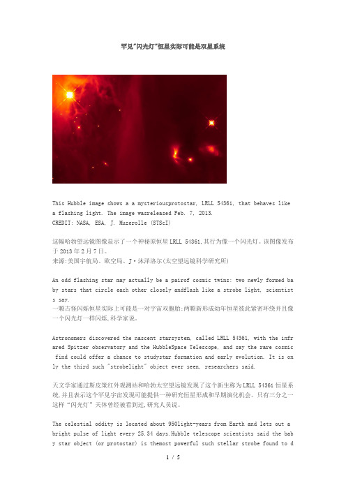
罕见"闪光灯"恒星实际可能是双星系统This Hubble image shows a a mysteriousprotostar, LRLL 54361, that behaves like a flashing light. The image wasreleased Feb. 7, 2013.CREDIT: NASA, ESA, J. Muzerolle (STScI)这幅哈勃望远镜图像显示了一个神秘原恒星LRLL 54361,其行为像一个闪光灯。

该图像发布于2013年2月7日。

来源:美国宇航局、欧空局、J·沐泽洛尔(太空望远镜科学研究所)An odd flashing star may actually be a pairof cosmic twins: two newly formed ba by stars that circle each other closely andflash like a strobe light, scientist s say.一颗古怪闪烁恒星实际上可能是一对宇宙双胞胎:两颗新形成幼年恒星彼此紧密环绕并且像一个闪光灯一样闪烁,科学家说。

Astronomers discovered the nascent starsystem, called LRLL 54361, with the infr ared Spitzer observatory and the HubbleSpace Telescope, and say the rare cosmic find could offer a chance to studystar formation and early evolution. It is on ly the third such "strobelight" object ever seen, researchers said.天文学家通过斯皮策红外观测站和哈勃太空望远镜发现了这个新生称为LRLL 54361恒星系统,并且表示这个罕见宇宙发现可能提供一种研究恒星形成和早期演化机会。

华中师范大学物理学院物理学专业英语仅供内部学习参考！2014一、课程的任务和教学目的通过学习《物理学专业英语》，学生将掌握物理学领域使用频率较高的专业词汇和表达方法，进而具备基本的阅读理解物理学专业文献的能力。

通过分析《物理学专业英语》课程教材中的范文，学生还将从英语角度理解物理学中个学科的研究内容和主要思想，提高学生的专业英语能力和了解物理学研究前沿的能力。

培养专业英语阅读能力，了解科技英语的特点，提高专业外语的阅读质量和阅读速度；掌握一定量的本专业英文词汇，基本达到能够独立完成一般性本专业外文资料的阅读；达到一定的笔译水平。

要求译文通顺、准确和专业化。

要求译文通顺、准确和专业化。

二、课程内容课程内容包括以下章节：物理学、经典力学、热力学、电磁学、光学、原子物理、统计力学、量子力学和狭义相对论三、基本要求1.充分利用课内时间保证充足的阅读量（约1200~1500词/学时），要求正确理解原文。

2.泛读适量课外相关英文读物，要求基本理解原文主要内容。

3.掌握基本专业词汇（不少于200词）。

4.应具有流利阅读、翻译及赏析专业英语文献，并能简单地进行写作的能力。

四、参考书目录1 Physics 物理学 (1)Introduction to physics (1)Classical and modern physics (2)Research fields (4)V ocabulary (7)2 Classical mechanics 经典力学 (10)Introduction (10)Description of classical mechanics (10)Momentum and collisions (14)Angular momentum (15)V ocabulary (16)3 Thermodynamics 热力学 (18)Introduction (18)Laws of thermodynamics (21)System models (22)Thermodynamic processes (27)Scope of thermodynamics (29)V ocabulary (30)4 Electromagnetism 电磁学 (33)Introduction (33)Electrostatics (33)Magnetostatics (35)Electromagnetic induction (40)V ocabulary (43)5 Optics 光学 (45)Introduction (45)Geometrical optics (45)Physical optics (47)Polarization (50)V ocabulary (51)6 Atomic physics 原子物理 (52)Introduction (52)Electronic configuration (52)Excitation and ionization (56)V ocabulary (59)7 Statistical mechanics 统计力学 (60)Overview (60)Fundamentals (60)Statistical ensembles (63)V ocabulary (65)8 Quantum mechanics 量子力学 (67)Introduction (67)Mathematical formulations (68)Quantization (71)Wave-particle duality (72)Quantum entanglement (75)V ocabulary (77)9 Special relativity 狭义相对论 (79)Introduction (79)Relativity of simultaneity (80)Lorentz transformations (80)Time dilation and length contraction (81)Mass-energy equivalence (82)Relativistic energy-momentum relation (86)V ocabulary (89)正文标记说明：蓝色Arial字体（例如energy）：已知的专业词汇蓝色Arial字体加下划线（例如electromagnetism）：新学的专业词汇黑色Times New Roman字体加下划线（例如postulate）：新学的普通词汇1 Physics 物理学1 Physics 物理学Introduction to physicsPhysics is a part of natural philosophy and a natural science that involves the study of matter and its motion through space and time, along with related concepts such as energy and force. More broadly, it is the general analysis of nature, conducted in order to understand how the universe behaves.Physics is one of the oldest academic disciplines, perhaps the oldest through its inclusion of astronomy. Over the last two millennia, physics was a part of natural philosophy along with chemistry, certain branches of mathematics, and biology, but during the Scientific Revolution in the 17th century, the natural sciences emerged as unique research programs in their own right. Physics intersects with many interdisciplinary areas of research, such as biophysics and quantum chemistry,and the boundaries of physics are not rigidly defined. New ideas in physics often explain the fundamental mechanisms of other sciences, while opening new avenues of research in areas such as mathematics and philosophy.Physics also makes significant contributions through advances in new technologies that arise from theoretical breakthroughs. For example, advances in the understanding of electromagnetism or nuclear physics led directly to the development of new products which have dramatically transformed modern-day society, such as television, computers, domestic appliances, and nuclear weapons; advances in thermodynamics led to the development of industrialization; and advances in mechanics inspired the development of calculus.Core theoriesThough physics deals with a wide variety of systems, certain theories are used by all physicists. Each of these theories were experimentally tested numerous times and found correct as an approximation of nature (within a certain domain of validity).For instance, the theory of classical mechanics accurately describes the motion of objects, provided they are much larger than atoms and moving at much less than the speed of light. These theories continue to be areas of active research, and a remarkable aspect of classical mechanics known as chaos was discovered in the 20th century, three centuries after the original formulation of classical mechanics by Isaac Newton (1642–1727) 【艾萨克·牛顿】.University PhysicsThese central theories are important tools for research into more specialized topics, and any physicist, regardless of his or her specialization, is expected to be literate in them. These include classical mechanics, quantum mechanics, thermodynamics and statistical mechanics, electromagnetism, and special relativity.Classical and modern physicsClassical mechanicsClassical physics includes the traditional branches and topics that were recognized and well-developed before the beginning of the 20th century—classical mechanics, acoustics, optics, thermodynamics, and electromagnetism.Classical mechanics is concerned with bodies acted on by forces and bodies in motion and may be divided into statics (study of the forces on a body or bodies at rest), kinematics (study of motion without regard to its causes), and dynamics (study of motion and the forces that affect it); mechanics may also be divided into solid mechanics and fluid mechanics (known together as continuum mechanics), the latter including such branches as hydrostatics, hydrodynamics, aerodynamics, and pneumatics.Acoustics is the study of how sound is produced, controlled, transmitted and received. Important modern branches of acoustics include ultrasonics, the study of sound waves of very high frequency beyond the range of human hearing; bioacoustics the physics of animal calls and hearing, and electroacoustics, the manipulation of audible sound waves using electronics.Optics, the study of light, is concerned not only with visible light but also with infrared and ultraviolet radiation, which exhibit all of the phenomena of visible light except visibility, e.g., reflection, refraction, interference, diffraction, dispersion, and polarization of light.Heat is a form of energy, the internal energy possessed by the particles of which a substance is composed; thermodynamics deals with the relationships between heat and other forms of energy.Electricity and magnetism have been studied as a single branch of physics since the intimate connection between them was discovered in the early 19th century; an electric current gives rise to a magnetic field and a changing magnetic field induces an electric current. Electrostatics deals with electric charges at rest, electrodynamics with moving charges, and magnetostatics with magnetic poles at rest.Modern PhysicsClassical physics is generally concerned with matter and energy on the normal scale of1 Physics 物理学observation, while much of modern physics is concerned with the behavior of matter and energy under extreme conditions or on the very large or very small scale.For example, atomic and nuclear physics studies matter on the smallest scale at which chemical elements can be identified.The physics of elementary particles is on an even smaller scale, as it is concerned with the most basic units of matter; this branch of physics is also known as high-energy physics because of the extremely high energies necessary to produce many types of particles in large particle accelerators. On this scale, ordinary, commonsense notions of space, time, matter, and energy are no longer valid.The two chief theories of modern physics present a different picture of the concepts of space, time, and matter from that presented by classical physics.Quantum theory is concerned with the discrete, rather than continuous, nature of many phenomena at the atomic and subatomic level, and with the complementary aspects of particles and waves in the description of such phenomena.The theory of relativity is concerned with the description of phenomena that take place in a frame of reference that is in motion with respect to an observer; the special theory of relativity is concerned with relative uniform motion in a straight line and the general theory of relativity with accelerated motion and its connection with gravitation.Both quantum theory and the theory of relativity find applications in all areas of modern physics.Difference between classical and modern physicsWhile physics aims to discover universal laws, its theories lie in explicit domains of applicability. Loosely speaking, the laws of classical physics accurately describe systems whose important length scales are greater than the atomic scale and whose motions are much slower than the speed of light. Outside of this domain, observations do not match their predictions.Albert Einstein【阿尔伯特·爱因斯坦】contributed the framework of special relativity, which replaced notions of absolute time and space with space-time and allowed an accurate description of systems whose components have speeds approaching the speed of light.Max Planck【普朗克】, Erwin Schrödinger【薛定谔】, and others introduced quantum mechanics, a probabilistic notion of particles and interactions that allowed an accurate description of atomic and subatomic scales.Later, quantum field theory unified quantum mechanics and special relativity.General relativity allowed for a dynamical, curved space-time, with which highly massiveUniversity Physicssystems and the large-scale structure of the universe can be well-described. General relativity has not yet been unified with the other fundamental descriptions; several candidate theories of quantum gravity are being developed.Research fieldsContemporary research in physics can be broadly divided into condensed matter physics; atomic, molecular, and optical physics; particle physics; astrophysics; geophysics and biophysics. Some physics departments also support research in Physics education.Since the 20th century, the individual fields of physics have become increasingly specialized, and today most physicists work in a single field for their entire careers. "Universalists" such as Albert Einstein (1879–1955) and Lev Landau (1908–1968)【列夫·朗道】, who worked in multiple fields of physics, are now very rare.Condensed matter physicsCondensed matter physics is the field of physics that deals with the macroscopic physical properties of matter. In particular, it is concerned with the "condensed" phases that appear whenever the number of particles in a system is extremely large and the interactions between them are strong.The most familiar examples of condensed phases are solids and liquids, which arise from the bonding by way of the electromagnetic force between atoms. More exotic condensed phases include the super-fluid and the Bose–Einstein condensate found in certain atomic systems at very low temperature, the superconducting phase exhibited by conduction electrons in certain materials,and the ferromagnetic and antiferromagnetic phases of spins on atomic lattices.Condensed matter physics is by far the largest field of contemporary physics.Historically, condensed matter physics grew out of solid-state physics, which is now considered one of its main subfields. The term condensed matter physics was apparently coined by Philip Anderson when he renamed his research group—previously solid-state theory—in 1967. In 1978, the Division of Solid State Physics of the American Physical Society was renamed as the Division of Condensed Matter Physics.Condensed matter physics has a large overlap with chemistry, materials science, nanotechnology and engineering.Atomic, molecular and optical physicsAtomic, molecular, and optical physics (AMO) is the study of matter–matter and light–matter interactions on the scale of single atoms and molecules.1 Physics 物理学The three areas are grouped together because of their interrelationships, the similarity of methods used, and the commonality of the energy scales that are relevant. All three areas include both classical, semi-classical and quantum treatments; they can treat their subject from a microscopic view (in contrast to a macroscopic view).Atomic physics studies the electron shells of atoms. Current research focuses on activities in quantum control, cooling and trapping of atoms and ions, low-temperature collision dynamics and the effects of electron correlation on structure and dynamics. Atomic physics is influenced by the nucleus (see, e.g., hyperfine splitting), but intra-nuclear phenomena such as fission and fusion are considered part of high-energy physics.Molecular physics focuses on multi-atomic structures and their internal and external interactions with matter and light.Optical physics is distinct from optics in that it tends to focus not on the control of classical light fields by macroscopic objects, but on the fundamental properties of optical fields and their interactions with matter in the microscopic realm.High-energy physics (particle physics) and nuclear physicsParticle physics is the study of the elementary constituents of matter and energy, and the interactions between them.In addition, particle physicists design and develop the high energy accelerators,detectors, and computer programs necessary for this research. The field is also called "high-energy physics" because many elementary particles do not occur naturally, but are created only during high-energy collisions of other particles.Currently, the interactions of elementary particles and fields are described by the Standard Model.●The model accounts for the 12 known particles of matter (quarks and leptons) thatinteract via the strong, weak, and electromagnetic fundamental forces.●Dynamics are described in terms of matter particles exchanging gauge bosons (gluons,W and Z bosons, and photons, respectively).●The Standard Model also predicts a particle known as the Higgs boson. In July 2012CERN, the European laboratory for particle physics, announced the detection of a particle consistent with the Higgs boson.Nuclear Physics is the field of physics that studies the constituents and interactions of atomic nuclei. The most commonly known applications of nuclear physics are nuclear power generation and nuclear weapons technology, but the research has provided application in many fields, including those in nuclear medicine and magnetic resonance imaging, ion implantation in materials engineering, and radiocarbon dating in geology and archaeology.University PhysicsAstrophysics and Physical CosmologyAstrophysics and astronomy are the application of the theories and methods of physics to the study of stellar structure, stellar evolution, the origin of the solar system, and related problems of cosmology. Because astrophysics is a broad subject, astrophysicists typically apply many disciplines of physics, including mechanics, electromagnetism, statistical mechanics, thermodynamics, quantum mechanics, relativity, nuclear and particle physics, and atomic and molecular physics.The discovery by Karl Jansky in 1931 that radio signals were emitted by celestial bodies initiated the science of radio astronomy. Most recently, the frontiers of astronomy have been expanded by space exploration. Perturbations and interference from the earth's atmosphere make space-based observations necessary for infrared, ultraviolet, gamma-ray, and X-ray astronomy.Physical cosmology is the study of the formation and evolution of the universe on its largest scales. Albert Einstein's theory of relativity plays a central role in all modern cosmological theories. In the early 20th century, Hubble's discovery that the universe was expanding, as shown by the Hubble diagram, prompted rival explanations known as the steady state universe and the Big Bang.The Big Bang was confirmed by the success of Big Bang nucleo-synthesis and the discovery of the cosmic microwave background in 1964. The Big Bang model rests on two theoretical pillars: Albert Einstein's general relativity and the cosmological principle (On a sufficiently large scale, the properties of the Universe are the same for all observers). Cosmologists have recently established the ΛCDM model (the standard model of Big Bang cosmology) of the evolution of the universe, which includes cosmic inflation, dark energy and dark matter.Current research frontiersIn condensed matter physics, an important unsolved theoretical problem is that of high-temperature superconductivity. Many condensed matter experiments are aiming to fabricate workable spintronics and quantum computers.In particle physics, the first pieces of experimental evidence for physics beyond the Standard Model have begun to appear. Foremost among these are indications that neutrinos have non-zero mass. These experimental results appear to have solved the long-standing solar neutrino problem, and the physics of massive neutrinos remains an area of active theoretical and experimental research. Particle accelerators have begun probing energy scales in the TeV range, in which experimentalists are hoping to find evidence for the super-symmetric particles, after discovery of the Higgs boson.Theoretical attempts to unify quantum mechanics and general relativity into a single theory1 Physics 物理学of quantum gravity, a program ongoing for over half a century, have not yet been decisively resolved. The current leading candidates are M-theory, superstring theory and loop quantum gravity.Many astronomical and cosmological phenomena have yet to be satisfactorily explained, including the existence of ultra-high energy cosmic rays, the baryon asymmetry, the acceleration of the universe and the anomalous rotation rates of galaxies.Although much progress has been made in high-energy, quantum, and astronomical physics, many everyday phenomena involving complexity, chaos, or turbulence are still poorly understood. Complex problems that seem like they could be solved by a clever application of dynamics and mechanics remain unsolved; examples include the formation of sand-piles, nodes in trickling water, the shape of water droplets, mechanisms of surface tension catastrophes, and self-sorting in shaken heterogeneous collections.These complex phenomena have received growing attention since the 1970s for several reasons, including the availability of modern mathematical methods and computers, which enabled complex systems to be modeled in new ways. Complex physics has become part of increasingly interdisciplinary research, as exemplified by the study of turbulence in aerodynamics and the observation of pattern formation in biological systems.Vocabulary★natural science 自然科学academic disciplines 学科astronomy 天文学in their own right 凭他们本身的实力intersects相交，交叉interdisciplinary交叉学科的，跨学科的★quantum 量子的theoretical breakthroughs 理论突破★electromagnetism 电磁学dramatically显著地★thermodynamics热力学★calculus微积分validity★classical mechanics 经典力学chaos 混沌literate 学者★quantum mechanics量子力学★thermodynamics and statistical mechanics热力学与统计物理★special relativity狭义相对论is concerned with 关注，讨论，考虑acoustics 声学★optics 光学statics静力学at rest 静息kinematics运动学★dynamics动力学ultrasonics超声学manipulation 操作，处理，使用University Physicsinfrared红外ultraviolet紫外radiation辐射reflection 反射refraction 折射★interference 干涉★diffraction 衍射dispersion散射★polarization 极化，偏振internal energy 内能Electricity电性Magnetism 磁性intimate 亲密的induces 诱导，感应scale尺度★elementary particles基本粒子★high-energy physics 高能物理particle accelerators 粒子加速器valid 有效的，正当的★discrete离散的continuous 连续的complementary 互补的★frame of reference 参照系★the special theory of relativity 狭义相对论★general theory of relativity 广义相对论gravitation 重力，万有引力explicit 详细的，清楚的★quantum field theory 量子场论★condensed matter physics凝聚态物理astrophysics天体物理geophysics地球物理Universalist博学多才者★Macroscopic宏观Exotic奇异的★Superconducting 超导Ferromagnetic铁磁质Antiferromagnetic 反铁磁质★Spin自旋Lattice 晶格，点阵，网格★Society社会，学会★microscopic微观的hyperfine splitting超精细分裂fission分裂，裂变fusion熔合，聚变constituents成分，组分accelerators加速器detectors 检测器★quarks夸克lepton 轻子gauge bosons规范玻色子gluons胶子★Higgs boson希格斯玻色子CERN欧洲核子研究中心★Magnetic Resonance Imaging磁共振成像，核磁共振ion implantation 离子注入radiocarbon dating放射性碳年代测定法geology地质学archaeology考古学stellar 恒星cosmology宇宙论celestial bodies 天体Hubble diagram 哈勃图Rival竞争的★Big Bang大爆炸nucleo-synthesis核聚合，核合成pillar支柱cosmological principle宇宙学原理ΛCDM modelΛ-冷暗物质模型cosmic inflation宇宙膨胀1 Physics 物理学fabricate制造，建造spintronics自旋电子元件，自旋电子学★neutrinos 中微子superstring 超弦baryon重子turbulence湍流，扰动，骚动catastrophes突变，灾变，灾难heterogeneous collections异质性集合pattern formation模式形成University Physics2 Classical mechanics 经典力学IntroductionIn physics, classical mechanics is one of the two major sub-fields of mechanics, which is concerned with the set of physical laws describing the motion of bodies under the action of a system of forces. The study of the motion of bodies is an ancient one, making classical mechanics one of the oldest and largest subjects in science, engineering and technology.Classical mechanics describes the motion of macroscopic objects, from projectiles to parts of machinery, as well as astronomical objects, such as spacecraft, planets, stars, and galaxies. Besides this, many specializations within the subject deal with gases, liquids, solids, and other specific sub-topics.Classical mechanics provides extremely accurate results as long as the domain of study is restricted to large objects and the speeds involved do not approach the speed of light. When the objects being dealt with become sufficiently small, it becomes necessary to introduce the other major sub-field of mechanics, quantum mechanics, which reconciles the macroscopic laws of physics with the atomic nature of matter and handles the wave–particle duality of atoms and molecules. In the case of high velocity objects approaching the speed of light, classical mechanics is enhanced by special relativity. General relativity unifies special relativity with Newton's law of universal gravitation, allowing physicists to handle gravitation at a deeper level.The initial stage in the development of classical mechanics is often referred to as Newtonian mechanics, and is associated with the physical concepts employed by and the mathematical methods invented by Newton himself, in parallel with Leibniz【莱布尼兹】, and others.Later, more abstract and general methods were developed, leading to reformulations of classical mechanics known as Lagrangian mechanics and Hamiltonian mechanics. These advances were largely made in the 18th and 19th centuries, and they extend substantially beyond Newton's work, particularly through their use of analytical mechanics. Ultimately, the mathematics developed for these were central to the creation of quantum mechanics.Description of classical mechanicsThe following introduces the basic concepts of classical mechanics. For simplicity, it often2 Classical mechanics 经典力学models real-world objects as point particles, objects with negligible size. The motion of a point particle is characterized by a small number of parameters: its position, mass, and the forces applied to it.In reality, the kind of objects that classical mechanics can describe always have a non-zero size. (The physics of very small particles, such as the electron, is more accurately described by quantum mechanics). Objects with non-zero size have more complicated behavior than hypothetical point particles, because of the additional degrees of freedom—for example, a baseball can spin while it is moving. However, the results for point particles can be used to study such objects by treating them as composite objects, made up of a large number of interacting point particles. The center of mass of a composite object behaves like a point particle.Classical mechanics uses common-sense notions of how matter and forces exist and interact. It assumes that matter and energy have definite, knowable attributes such as where an object is in space and its speed. It also assumes that objects may be directly influenced only by their immediate surroundings, known as the principle of locality.In quantum mechanics objects may have unknowable position or velocity, or instantaneously interact with other objects at a distance.Position and its derivativesThe position of a point particle is defined with respect to an arbitrary fixed reference point, O, in space, usually accompanied by a coordinate system, with the reference point located at the origin of the coordinate system. It is defined as the vector r from O to the particle.In general, the point particle need not be stationary relative to O, so r is a function of t, the time elapsed since an arbitrary initial time.In pre-Einstein relativity (known as Galilean relativity), time is considered an absolute, i.e., the time interval between any given pair of events is the same for all observers. In addition to relying on absolute time, classical mechanics assumes Euclidean geometry for the structure of space.Velocity and speedThe velocity, or the rate of change of position with time, is defined as the derivative of the position with respect to time. In classical mechanics, velocities are directly additive and subtractive as vector quantities; they must be dealt with using vector analysis.When both objects are moving in the same direction, the difference can be given in terms of speed only by ignoring direction.University PhysicsAccelerationThe acceleration , or rate of change of velocity, is the derivative of the velocity with respect to time (the second derivative of the position with respect to time).Acceleration can arise from a change with time of the magnitude of the velocity or of the direction of the velocity or both . If only the magnitude v of the velocity decreases, this is sometimes referred to as deceleration , but generally any change in the velocity with time, including deceleration, is simply referred to as acceleration.Inertial frames of referenceWhile the position and velocity and acceleration of a particle can be referred to any observer in any state of motion, classical mechanics assumes the existence of a special family of reference frames in terms of which the mechanical laws of nature take a comparatively simple form. These special reference frames are called inertial frames .An inertial frame is such that when an object without any force interactions (an idealized situation) is viewed from it, it appears either to be at rest or in a state of uniform motion in a straight line. This is the fundamental definition of an inertial frame. They are characterized by the requirement that all forces entering the observer's physical laws originate in identifiable sources (charges, gravitational bodies, and so forth).A non-inertial reference frame is one accelerating with respect to an inertial one, and in such a non-inertial frame a particle is subject to acceleration by fictitious forces that enter the equations of motion solely as a result of its accelerated motion, and do not originate in identifiable sources. These fictitious forces are in addition to the real forces recognized in an inertial frame.A key concept of inertial frames is the method for identifying them. For practical purposes, reference frames that are un-accelerated with respect to the distant stars are regarded as good approximations to inertial frames.Forces; Newton's second lawNewton was the first to mathematically express the relationship between force and momentum . Some physicists interpret Newton's second law of motion as a definition of force and mass, while others consider it a fundamental postulate, a law of nature. Either interpretation has the same mathematical consequences, historically known as "Newton's Second Law":a m t v m t p F ===d )(d d dThe quantity m v is called the (canonical ) momentum . The net force on a particle is thus equal to rate of change of momentum of the particle with time.So long as the force acting on a particle is known, Newton's second law is sufficient to。

a rXiv:as tr o-ph/21645v21Nov22A Submillimeter and Radio Survey of Gamma-Ray Burst Host Galaxies:A Glimpse into the Future of Star Formation Studies E.Berger 1,L.L.Cowie 2,S.R.Kulkarni 1,D.A.Frail 3,H.Aussel 2,&A.J.Barger 2,4,5ABSTRACT We present the first comprehensive search for submillimeter and radio emis-sion from the host galaxies of twenty well-localized γ-ray bursts (GRBs).With the exception of a single source,all observations were undertaken months to years after the GRB explosions to ensure negligible contamination from the afterglows.We detect the host galaxy of GRB 000418in both the sub-mm and radio,and the host galaxy of GRB 000210only in the sub-mm.These observations,in con-junction with the previous detections of the host galaxies of GRB 980703and GRB 010222,indicate that about 20%of GRB host galaxies are ultra-luminous (L >1012L ⊙)and have star formation rates of about 500M ⊙yr −1.As an en-semble,the non-detected hosts have a star formation rate of about 100M ⊙yr −1(5σ)based on their radio emission.The detected and ensemble star formation rates exceed the optically-determined values by an order of magnitude,indicat-ing significant dust obscuration.In the same vein,the ratio of bolometric dust luminosity to UV luminosity for the hosts detected in the sub-mm and radio ranges from ∼20−800,and follows the known trend of increasing obscuration with increasing bolometric luminosity.We also show that,both as a sample and individually,the GRB host galaxies have bluer R −K colors as compared with galaxies selected in the sub-mm in the same redshift range.This possibly in-dicates that the stellar populations in the GRB hosts are on average younger,supporting the massive stellar progenitor scenario for GRBs,but it is also possible that GRB hosts are on average less dusty.Beyond the specific results presentedin this paper,the sub-mm and radio observations serve as an observational proof-of-concept in anticipation of the upcoming launch of the SWIFT GRB missionand SIRTF.These new facilities will possibly bring GRB host galaxies into theforefront of star formation studies.Subject headings:cosmology:observations—galaxies:starburst—gamma-rays:bursts—stars:formation1.IntroductionOne of the major thrusts in modern cosmology is an accurate census of star formation and star-forming galaxies in the Universe.This endeavor forms the backbone for a slew of methods(observational,analytical,and numerical)to study the process of galaxy formation and evolution over cosmic time.To date,star-forming galaxies have been selected and studied mainly in two observational windows:the rest-frame ultraviolet(UV),and rest-frame radio and far-infrared(FIR).For galaxies at high redshift these bands are shifted into the optical and radio/sub-mm,allowing observations from the ground.Still,the problem of translating the observed emission to star formation rate(SFR)involves large uncertainty.This is partly because each band traces only a minor portion of the total energy output of stars.Moreover, the optical/UV band is significantly affected by dust obscuration,thus requiring order of magnitude corrections,while the sub-mm and radio bands lack sensitivity,and therefore uncover only the most prodigiously star-forming galaxies.The main result that has emerged from star formation surveys over the past few years is exemplified in the so-called Madau ly,the SFR volume density,ρSFR(z), rises steeply to z∼1,and seemingly peaks at z∼1−2.There is still some debate about the how steep the rise is,with values ranging from(1+z)1.5(Wilson et al.2002)to(1+z)4 (e.g.Madau et al.1996).The evolution beyond z∼2is even less clear since optical/UV observations indicate a decline(Madau et al.1996),while recent sub-mm observations argue for aflatρSFR(z)to higher redshift,z∼4(Barger,Cowie&Richards2000).Consistency with this trend can be obtained by invoking large dust corrections in the optical/UV(Steidel et al.1999).For general reviews of star formation surveys we refer the reader to Kennicut (1998),Adelberger&Steidel(2000),and Blain et al.(2002).Despite the significant progress in thisfield,our current understanding of star formation and its redshift evolution is still limited by the biases and shortcomings of current optical/UV, sub-mm,and radio selection techniques.In particular,despite the fact that the optical/UV band is sensitive to galaxies with modest star formation rates(down to a fraction of a M⊙yr−1)at high redshift,these surveys may miss the most dusty,and vigorously star-forming galaxies.Moreover,it is not clear if the simple,locally-calibrated prescriptions for correcting the observed un-obscured SFR for dust extinction(e.g.Meurer,Heckman&Calzetti1999), hold at high redshift;even if they do,these prescriptions involve an order of magnitude correction.Finally,the optical/UV surveys are magnitude limited,and therefore miss the faintest sources.Sub-mm surveys have uncovered a population of highly dust-extincted galaxies,which are usually optically faint,and have star formation rates of several hundred M⊙yr−1(e.g.Smail, Ivison&Blain1997).However,unlike optical/UV surveys,sub-mm surveys are severely sen-sitivity limited,and only detect galaxies with L bol 1012L⊙.More importantly,current sub-mm bolometer arrays(such as SCUBA)have large beams on the sky(∼15arcsec) making it difficult to unambiguously identify optical counterparts(which are usually faint to begin with),and hence measure the redshifts(Smail et al.2002);in fact,of the∼200 sub-mm galaxies identified to date,only a handful have a measured redshift.Finally,trans-lating the observed sub-mm emission to a SFR requires significant assumptions about the temperature of the dust,and the dust emission spectrum(e.g.Blain et al.2002).Surveys at decimeter radio wavelengths also suffer from low sensitivity,but the high as-trometric accuracy afforded by synthesis arrays such as the VLA allows a sub-arcsec localiza-tion of the radio-selected galaxies.As a result,it is easier to identify the optical counterparts of these sources.Recently,this approach has been used to pre-select sources for targeted sub-mm observations resulting in an increase in the sub-mm detection rate(Barger,Cowie &Richards2000;Chapman et al.2002)and redshift determination(Chapman et al.2003). However,this method is biased towardfinding luminous(high SFR)sources since it requires an initial radio detection.An additional problem with radio,even more than with sub-mm, selection is contamination by active galactic nuclei(AGN).An examination of the X-ray properties of radio and sub-mm selected galaxies reveals that of the order of20%can have a significant AGN component(Barger et al.2001).The most significant problem with current star formation studies,however,is that the link between the optical and sub-mm/radio samples is still not well understood.The Hubble Deep Field provides a clear illustration:the brightest sub-mm source does not appear to have an optical counterpart(Hughes et al.1998),and only recently a detection has been claimed in the near-IR(K≈23.5mag;Dunlop et al.2002).Along the same line,sub-mm observations of the optically-selected Lyman break galaxies have resulted in very few detections(Chapman et al.2000;Peacock et al.2000;Chapman et al.2002),and even the brightest Lyman break galaxies appear to be faint in the sub-mm band(Baker et al. 2001).In addition,there is considerable diversity in the properties of optical counterpartsto sub-mm sources,ranging from galaxies which are faint in both the optical and near-IR (NIR)to those which are bright in both bands(Ivison et al.2000;Smail et al.2002).As a result of the unclear overlap,and the sensitivity and dust problems in the sub-mm and optical surveys,the fractions of global star formation in the optical and sub-mm/radio selected galaxies is not well constrained.It is therefore not clear if the majority of star formation takes place in ultra-luminous galaxies with very high star formation rates,or in the more abundant lower luminosity galaxies with star formation rates of a few M⊙yr−1. Given the difficulty with redshift identification of sub-mm galaxies,the redshift distribution of dusty star forming galaxies remains highly uncertain.One way to alleviate some of these problems is to study a sample of galaxies that is immune to the selection biases of current optical/UV and sub-mm/radio surveys,and which may draw a more representative sample of the underlying distribution of star-forming galaxies.The host galaxies ofγ-ray bursts(GRBs)may provide one such sample.The main advantages of the sample of GRB host galaxies are:(i)The galaxies are selected with no regard to their emission properties in any wavelength regime,(ii)the dust-penetrating power of theγ-ray emission results in a sample that is completely unbiased with respect to the global dust properties of the hosts,(iii)GRBs can be observed to very high redshifts with existing missions(z 10;Lamb&Reichart2000),and as a result volume corrections for the star formation rates inferred from their hosts are trivial,(iv)the redshift of the galaxy can be determined via absorption spectroscopy of the optical afterglow,or X-ray spectroscopy allowing a redshift measurement of arbitrarily faint galaxies(the current record-holder is the host of GRB990510with R=28.5mag and z=1.619;Vreeswijk et al.2001),and(v)since there is excellent circumstantial evidence linking GRBs to massive stars(e.g.Bloom,Kulkarni&Djorgovski2002,the sample of GRB hosts is expected to trace global star formation(Blain&Natarajan2000).Of course,the sample of GRB hosts is not immune from its own problems and potential biases.The main problem is the relatively small size of the sample in comparison to both the optical and sub-mm samples6(although the number of GRB hosts with a known redshift exceeds the number of sub-mm galaxies with a measured redshift).As a result,at the present it is not possible to assess the SFR density that is implied by GRB hosts,or its redshift evolution.A bias towards sub-solar metallicity for GRB progenitors(and hence their environments)has been discussed(MacFadyen&Woosley1999;MacFadyen,Woosley &Heger2001),but it appears that very massive stars(e.g.M 35M⊙)should produceblack holes even at solar metallicity.The impact of metallicity on additional aspects of GRB formation(e.g.angular momentum,loss of hydrogen envelope)is not clear at present. Finally,given the observed dispersion in metallicity within galaxies(e.g.Alard2001;Overzier et al.2001),it is likely that even if GRBs require low metallicity progenitors,this does not imply that the galaxy as a whole has a lower than average metallicity.To date,GRB host galaxies have mainly been studied in the optical and NIR bands. With the exception of one source(GRB020124;Berger et al.2002),every GRB localized to a sub-arcsecond position has been associated with a star-forming galaxy(Bloom,Kulkarni &Djorgovski2002).These galaxies range from R≈22−29mag,have a median redshift, z ∼1,and are generally typical of star-forming galaxies at similar redshifts in terms of morphology and luminosity(Djorgovski et al.2001),with star formation rates from optical spectroscopy of∼1−10M⊙yr−1.At the same time,there are hints for higher than average ratios of[Ne III]3869to[O II]3727,possibly indicating the presence of massive stars (Djorgovski et al.2001).Only two host galaxies have been detected so far in the radio (GRB980703;Berger,Kulkarni&Frail2001)and sub-mm(GRB010222;Frail et al.2002).Here we present sub-mm and radio observations of a sample of20GRB host galaxies, ranging in redshift from about0.4to4.5(§2);one of the20sources is detected with high significance in both the sub-mm and radio bands,and an additional source is detected in the sub-mm(§3).We compare the detected sub-mm and radio host galaxies to local and high-z ultra-luminous galaxies in§4,and derive the SFRs in§5.We then compare the inferred SFRs of the detected host galaxies,and the ensemble of undetected hosts,to optical estimates in §6.Finally,we compare the optical properties of the GRB host galaxies to those of sub-mm and radio selected star-forming galaxies(§7).2.Observations2.1.Target SelectionAt the time we conducted our survey,the sample of GRB host galaxies numbered25, twenty of which had measured redshifts.These host galaxies were localized primarily based on optical afterglows,but also using the radio and X-ray afterglow emission.Of the25host galaxies we observed eight in both the radio and sub-mm,seven in the radio,andfive in the sub-mm.The galaxies were drawn from the list of25hosts at random,constrained primarily by the availability of observing time.Thus,the sample presented here does not suffer from any obvious selection biases,with the exception of detectable afterglow emission in at least one band.Sub-mm observations of GRB afterglows,and a small number of host galaxies have been undertaken in the past.Starting in1997,Smith et al.(1999)and Smith et al.(2001)have searched for sub-mm emission from the afterglow of thirteen GRBs.While they did not detect any afterglow emission,these authors used their observations to place constraints on emission from eight host galaxies,with typical1σrms values of1.2mJy.Since these were target-of-opportunity observations,they were not always undertaken in favorable observing conditions.More recently,Barnard et al.(2002)reported targeted sub-mm observations of the host galaxies of four optically-dark GRBs(i.e.GRBs lacking an optical afterglow).They focused on these particular sources since one explanation for the lack of optical emission is obscuration by dust,which presumably points to a dusty host.None of the hosts were detected,with the possible exception of GRB000210(see§3.4),leading the authors to conclude that the hosts of dark bursts are not necessarily heavily dust obscured.Thus,the observations presented here provide the most comprehensive and bias-free search for sub-mm emission from GRB host galaxies,and thefirst comprehensive search for radio emission.2.2.Submillimeter ObservationsObservations in the sub-mm band were carried out using the Sub-millimeter Common User Bolometer Array(SCUBA;Holland et al.1999)on the James Clerk Maxwell Tele-scope(JCMT7).We observed the positions of thirteen well-localized GRB afterglows with the long(850µm)and short(450µm)arrays.The observations,summarized in Table1, were conducted in photometry mode with the standard nine-jiggle pattern using the central bolometer in each of the two arrays to observe the source.In the case of GRB000301C we used an off-center bolometer in each array due to high noise levels in the central bolometer.To account for variations in the sky brightness,we used a standard chopping of the secondary mirror between the on-source position and a position60arcsec away in azimuth, at a frequency of7.8125Hz.In addition,we used a two-position beam switch(nodding), in which the beam is moved off-source in each exposure to measure the sky.Measurements of the sky opacity(sky-dips)were taken approximately every two hours,and the focus andarray noise were checked at least twice during each shift.The pointing was checked approximately once per hour using several sources throughout each shift,and was generally found to vary by 3arcsec(i.e.less than one quarter of the beam size).All observations were performed in band2and3weather withτ225GHz≈0.05−0.12.The data were initially reduced with the SCUBA Data Reduction Facility(SURF)fol-lowing the standard reduction procedure.The off-position pointings were subtracted from the on-position pointings to account for chopping and nodding of the telescope.Noisy bolometers were removed to facilitate a more accurate sky subtraction(see below),and the data were thenflat-fielded to account for the small differences in bolometer response.Ex-tinction correction was performed using a linear interpolation between skydips taken before and after each set of on-source scans.In addition to the sky subtraction offered by the nodding and chopping,short-term sky contributions were subtracted by using all low-noise off-source bolometers(sky bolometers). This procedure takes advantage of the fact that the sky contribution is correlated across the array.As a result,theflux in the sky bolometers can be used to assess the sky contribution to theflux in the on-source bolometer.This procedure is especially crucial when observing weak sources,since the measuredflux may be dominated by the sky.We implemented the sky subtraction using SURF and our own routine using MATLAB.We found that in general the SURF sky subtraction under-estimated the sky contribution,and as a result over-estimated the sourcefluxes.We therefore used the results of our own analysis routine.For this purpose we calculated the median value of the two(three)outer rings of bolometers in the850µm (450µm)array,after removing noisy bolometers(defined as those whose standard deviation over a whole scan deviated by more than5σfrom the median standard deviation of all sky bolometers).Following the sky subtraction,we calculated the mean and standard deviation of the mean(SDOM)for each source in a given observing shift.Noisy data were eliminated in two ways.First,the data were binned into25equal time bins,and the SDOM was calculated step-wise,i.e.at each step the data from an additional bin were added and the mean and SDOM were re-calculated.In an ideal situation where the data quality remains approximately constant,the SDOM should progressively decrease as more data are accumulated.However, if the quality of the data worsens(due to deteriorating weather conditions for example) the SDOM will increase.We therefore removed time bins in which the SDOM increased. Following this procedure,we recursively eliminated individual noisy data points using a sigma cutofflevel based on the number of data points(Chauvenet’s criterion;Taylor1982)until the mean converged on a constant value.Typically,two or three iterations were required,with only a few data points rejected each time.Typically,only a few percent of the data were rejected by the two procedures.Finally,flux conversion factors(FCFs)were applied to the resulting voltage measure-ments to convert the signal to ing photometry observations of Mars and Uranus,and/or secondary calibrators(OH231.8+4.2,IRC+10216,and CRL618),we found the FCFto vary between180−205Jy/V at850µm,consistent with the typical value of197±13.At450µm,the FCFs varied between250−450Jy/V.2.3.Radio ObservationsVery Large Array(VLA8):We observed12GRB afterglow positions with the VLA from April2001to February2002.All sources were observed at8.46GHz in the standard continuum mode with2×50MHz bands.In addition,GRB000418was observed at1.43and4.86GHz,and GRB0010222was observed at4.86GHz.In Table2we provide a summaryof the observations.In principle,since the median spectrum of faint radio sources between1.4and8.5GHzis Fν∝ν−0.6(Fomalont et al.2002),the ideal VLA frequency for our observations(takinginto account the sensitivity at each frequency)is1.43GHz.However,we chose to observe primarily at8.46GHz for the following reason.The majority of our observations were takenin the BnC,C,CnD,and D configurations,in which the typical synthesized beam size is∼10−40arcsec at1.43GHz,compared to∼2−8arcsec at8.46GHz.The large synthesized beam at1.43GHz,combined with the largerfield of view and higher intrinsic brightnessof radio sources at this frequency,would result in a significant decrease in sensitivity dueto source confusion.Thus,we were forced to observe at higher frequencies,in which the reduced confusion noise more than compensates for the typical steep spectrum.We chose8.46GHz rather than4.86GHz since the combination of20%higher sensitivity and60% lower confusion noise,provide a more significant impact than the typical30%decrease in intrinsic brightness.The1.43GHz observations of GRB000418were undertaken in the Aconfiguration,where confusion does not play a limiting role.Forflux calibration we used the extragalactic sources3C48(J0137+331),3C147(J0542+498), and3C286(J1331+305),while the phases were monitored using calibrator sources within∼5◦of the survey sources.We used the Astronomical Image Processing System(AIPS)for data reduction and analysis.For each source we co-added all the observations prior to producing an image,to increase thefinal signal-to-noise.Australia Telescope Compact Array(ATCA9):We observed the positions of four GRB afterglows during April2002,in the6A configuration ing the6-km baseline resulted in a significant decrease in confusion noise,thus allowing observations at the most advantageous frequencies.The observations are summarized in Table2.We used J1934−638forflux calibration,while the phase was monitored using calibrator sources within∼5◦of the survey sources.The data were reduced and analyzed using the Multichannel Image Reconstruction,Image Analysis and Display(MIRIAD)package,and AIPS.3.ResultsTheflux measurements at the position of each GRB are given in Tables1and2,and are plotted in Figure2.Of the20sources,only GRB000418was detected in both the radio and sub-mm with S/N>3(§3.1).One additional source,GRB000210,is detected with S/N>3 when combining our observations with those of Barnard et al.(2002).Two hosts have radio fluxes with3<S/N<4(GRB000301C and GRB000926),but as we show below this is due in part to emission from the afterglow.The typical2σthresholds are about2mJy,20µJy,and70µJy in the SCUBA,VLA,and ATCA observations,respectively.In Figure2we plot all sources with S/N>3as detections, and the rest as2σupper limits.In addition,for the sources observed with the ATCA we plot both the1.4GHz upper limits,and the inferred upper limits at8.46GHz assuming a typical radio spectrum,Fν∝ν−0.6(Fomalont et al.2002).One obvious source for the observed radio and sub-mmfluxes(other than the putative host galaxies)is emission from the afterglows.To assess the possibility that our observa-tions are contaminated byflux from the afterglows we note that the observations have been undertaken at least a year after the GRB explosion10.On this timescale,the sub-mm emis-sion from the afterglow is expected to be much lower than the detection threshold of ourobservations.In fact,the brightest sub-mm afterglows to date have only reached aflux of a few mJy(at350GHz),and typically exhibited a fading rate of∼t−1after about one day following the burst(Smith et al.1999;Berger et al.2000;Smith et al.2001;Frail et al. 2002;Yost et al.2002).Thus,on the timescale of our observations,the expected sub-mm flux from the afterglows is only∼10µJy,well below the detection threshold.The radio emission from GRB afterglows is more long-lived,and hence posses a more serious problem.However,on the typical timescale of the radio observations the8.46GHz flux is expected to be at most a fewµJy(e.g.Berger et al.2000).In the following sections we discuss the individual detections in the radio and sub-mm, and also provide an estimate for the radio emission from each afterglow.3.1.GRB000418A source at the position of GRB000418is detected at four of thefive observing fre-quencies with S/N>3.The SCUBA source,which we designate SMM12252+2006,has a flux density of Fν(350GHz)≈3.2±0.9mJy,and Fν(670GHz)≈41±19mJy.These values(Fν∝νβ),consistent with a thermal dust spectrum as imply a spectral index,β≈3.9+1.1−1.3expected if the emission is due to obscured star formation.The radio source(VLA122519.26+200611.1),is located atα(J2000)=12h25m19.255s,δ(J2000)=20◦06′11.10′′,with an uncertainty of0.1arcsec in both coordinates.This position is offset from the position of the radio afterglow of GRB000418(Berger et al.2001)by ∆α=−0.40±0.14arcsec and∆δ=−0.04±0.17arcsec(Figure1).In comparison,the offset measured from Keck and Hubble Space Telescope images is smaller,∆α=−0.019±0.066 arcsec and∆δ=0.012±0.058arcsec.VLA122519.26+200611.1has an observed spectral slopeβ=−0.17±0.25,flatter than the typical value for faint radio galaxies,β≈−0.6(Fomalont et al.2002),and similar to the value measured for the host of GRB980703(β≈−0.32;Berger,Kulkarni&Frail2001). The source appears to be slightly extended at1.43and8.46GHz,with a size of about1 arcsec(8.8kpc at z=1.119).The expected afterglowfluxes at4.86and8.46GHz at the time of our observations are about5and10µJy,respectively(Berger et al.2001).At1.43GHz the afterglow contribution is expected to be about10µJy based on the4.86GHzflux and the afterglow spectrum Fν∝ν−0.65.Thus,despite the contribution from the afterglow,the radio detections of the host galaxy are still significant at better than3σlevel.Correcting for the afterglowcontribution wefind an actual spectral slopeβ=−0.29±0.33,consistent with the median β≈−0.6for8.46GHz radio sources with a similarflux(Fomalont et al.2002).As with all SCUBA detections,source confusion arising from the large beam(D FWHM≈14arcsec at350GHz and≈6arcsec at670GHz)raises the possibility that SMM12252+2006 is not associated with the host galaxy of GRB000418.Fortunately,the detection of the radio source,which is located0.4±0.1arcsec away from the position of the radio afterglow of GRB000418,indicates that SMM12252+2006and VLA122519.26+200611.1are in fact the same source—the host galaxy of GRB000418.Besides the positional coincidence of the VLA and SCUBA sources,we gain further.This confidence of the association based on the spectral index between the two bands,β3501.4 spectral index is redshift dependent as a result of the different spectral slopes in the two regimes(Carilli&Yun2000;Barger,Cowie&Richards2000).Wefindβ350≈0.73±0.10,1.4=0.59±0.16(for the redshift in good agreement with the Carilli&Yun(2000)value ofβ3501.4of GRB000418,z=1.119).We also detect another source,slightly extended(θ≈1arcsec),approximately1.4arcsec East and2.7arcsec South of the host of GRB000418(designated VLA122519.36+200608.4), with Fν(1.43GHz)=48±15µJy and Fν(8.46GHz)=37±12µJy(see Figure1).This source appears to be linked by a bridge of radio emission(with S/N≈1.5at both frequencies)to the host of GRB000418.The physical separation between the two sources,assuming both are at the same redshift,z=1.119,is25kpc.There is no obvious optical counterpart to this source in Hubble Space Telescope images down to about R∼27.5mag.Based purely on radio source counts at8.46GHz(Fomalont et al.2002),the expected number of sources with Fν(8.46GHz)≈37µJy in a3arcsec radius circle is only about 2.7×10−4.Thus,the coincidence of two such faint sources within3arcsec is highly suggestive of an interacting system,rather than chance superposition.Interacting radio galaxies with separations of about20kpc,and joined by a bridge of radio continuum emission have been observed locally(Condon et al.1993;Condon,Helou& Jarrett2002).In addition,optical surveys(e.g.Patton et al.2002)show that a few percent of galaxies with an absolute B-band magnitude similar to that of the host of GRB000418, have companions within about30kpc.The fraction of interacting systems is possibly much higher,∼50%,in ultra-luminous systems(such as the host of GRB000418),both locally (Sanders&Mirabel1996)and at high redshift(e.g.Ivison et al.2000).We note that with a separation of only3arcsec,the host of GRB000418and the companion galaxy fall within the SCUBA beam.Thus,it is possible that SMM12252+2006to about is in fact a superposition of both radio sources.This will change the value ofβ3501.4。

第19卷第6期 半　导　体　学　报 V o l.19,N o.6 1998年6月 CH I N ESE JOU RNAL O F SE M I CONDU CTOR S June,1998　掺施主杂质半导体中LO声子的反对称光电导响应的M on te Carlo模拟陈张海　陈忠辉　刘普霖　石晓红　史国良　胡灿明　沈学础(中国科学院上海技术物理研究所　红外物理国家重点实验室　上海　200083)摘要　本文基于一个伴随LO声子发射的光激发电子被重新俘获的物理模型,采用M on teCarlo方法,对掺施主杂质的半导体光电导谱中与LO声子相对应的反对称谱峰结构进行了理论模拟,并与Si掺杂的GaA s及InP的实验结果作了比较.PACC:7240,7155,6320,02701　引言在过去的几十年中,人们对掺杂半导体中光激发载流子与LO声子相互作用而引入的非本征光电导响应进行了广泛的研究[1～4].Stocker等人曾指出,在掺杂半导体的光电导测量中,从杂质能级上被入射光子激发到导带而引入的过剩热载流子,可通过级联地发射LO 声子而弛豫到导带底,并在所施加的电场方向上引起净动量损失[1～3].他们的这个模型可用来解释或预言光电导谱中发生在入射光子能量hΜ=E i+n∂ΞLO)(其中,E i为杂质电离能,∂ΞLO为LO声子能量,n为正整数)附近的“负微分(光)电导”(negative differen tial conduc2 tance)或所谓“完全的负电导”(to tal negative conductance)现象[1,3].他们通过解Bo ltz m ann 输运方程计算了这样的振荡光电导响应[2,3].不久,M ears等人在CdT e光电导谱中的n∂ΞLO)能量处也观察到电导极小值[4],他们认为,在这种情形下,光激发电子最终并不是弛豫到导带底,而是重新被杂质俘获.另一个与LO声子直接相关的实验现象是出现在GaA s 和InP的低温光电导谱中的一个LO声子能量处的反对称峰[5～7];结合Stocker等人动量损失模型和M ears等人的杂质俘获模型,这样的反对称光电导结构的物理起源可以得到定性的说明[6,7].在本文中,我们将采用M on te Carlo方法,对这一定性模型进行理论计算,进而直接获得LO声子反对称光电导峰的模拟线形,并与实验结果进行了比较.陈张海　男,1969年出生,博士,主要从事半导体磁光光谱研究1997204209收到,1998202213定稿2　物理模型一般来说,在一个LO 声子能量∂ΞLO 附近引入光电导响应的物理机制可以由图1示意给出.在低温下,当能量略高于∂ΞLO 的入射光子将杂质基态电子激发到导带而成为初始动能接近于∂ΞLO -E i (E i 为杂质电离能)的热载流子,x 方向的电场力将使具有-k x 波矢的电子减速.一旦其能量等于∂ΞLO -E i ,该电子将发射一个LO 声子而重新被杂质基态俘获.而具有k x 波矢的电子将在电场的作用下加速,从而更远离共振条件,它被杂质重新俘获的几率较小.这样的机制将导致如图1(a )下半部分所示的导带电子分布.可以看出,由于这些光激发电子在电场力的反方向上有一净动量损失,这时将检测到正的光电导信号.而当处于杂质基态的电子被能量略低于∂ΞLO 的入射光子激发到导带时,同样地,x 方向的电场力将使具有-k x 波矢的电子减速而使具有k x 波矢的电子加速,当其能量等于∂ΞLO -E i ,该电子将发射一个LO 声子而重新被杂质基态俘获.这也将导致光激发电子沿x 方向的不对称分布(图1(b )),并使得光激发电子在电场力方向上有一净动量损失,这样的机制将导致LO 声子低能侧负光电导的出现.图1　在LO 声子能量处产生正、负光电导响应机制的示意图3　M on te Carlo 模拟上述物理过程可以由Bo ltz m ann 输运方程定量描述,然而直接求解这种光激发电子体系的Bo ltz m ann 方程是十分困难的事情,并且很难得到精确解.因此,我们采用M on te Car 2lo 方法,对处于外电场下电子的随机运动直接进行模拟.在M on te Carlo 模拟过程中,一些物理量和物理过程,如电子的自由飞行时间、散射机制、散射后的电子状态等,需要进行随机确定或选择[8,9].由于我们要处理的是类似于与时间或空间分布有关的大量粒子的随机运动过程[8～11],因此,必须对多个独立电子的运动进行模拟,而某个感兴趣的物理量A 的平均值可以方便地由下式求得[0,11],A (t )=1N ∑N i =1A i (t )(1)这里　N 为粒子的个数.在计算过程中,我们以掺杂的作为模拟对象,并认为其位于布里渊区点的844 半　导　体　学　报　19卷导带能谷具有球形等能面,同时考虑了能带非抛物性的修正[8],即导带电子的动能E (k ο)和波矢k ο的关系满足∂2k ο22m 3=E (k ο)[1+ΑE (k ο)](2)这里　Α=[1-(m 3 m 0)] E g ,m 3和m 0分别为导带电子有效质量和电子的静质量,E g 为GaA s 的禁带宽度.在模拟程序中,我们考虑了电子的三种散射机制,即声学声子散射,LO 声子散射和电离杂质散射,并直接引用文献[8]和文献[9]中给出的有关这几种散射机制的散射率公式及主要模拟参数.由于光激发产生的电子浓度很小,同时考虑到光电导测量是在低温下进行,并且施加在半导体两端的电压也不高,因此,电子2电子散射和谷间散射可以忽略不计.导带电子的复合与产生均以一定的概率发生,在模拟过程中它们被当作两种特殊的散射机制.电子于两次散射之间在外电场作用下的自由运动由∂k ο=eE ψ(e 为电子电荷,E ψ为电场强度)确定.但是,一旦光激发电子的能量达到∂ΞLO -E i ,则停止对该电子的模拟,并记录它最后的状态.这对应于电子被杂质基态重新俘获的过程.由上述的M on te Carlo 模拟过程可以直接得电子的分布函数.图2给出了导带中光激发电子沿-k x 方向稳态分布的计算结果的两个例子,它们分别描述不存在外电场(实线)和图2　存在外电场(虚线)和没有外电场下(实线)导带中光激发电子稳态分布的模拟结果存在沿-k x 方向外电场(虚线)情形下初始动能E 0=h Μ-E i 小于LO 声子能量时的非平衡电子分布.由于在低温下,电子受到主要散射机制是与电离杂质的弹性碰撞,在这些非平衡载流子的存在期间,由声学声子或LO 声子散射引起的电子动能损失很小,因此,可以近似认为构成如图4所示的无外场情况下对称分布的电子具有相同的动能.而一旦沿-k x 方向加上电场,具有-k x 方向动量的电子将在电场力的作用下而降低动能,此时的电子分布将呈现不对称性.图3给出了电场强度为50V c m 时、初始动能在∂ΞLO -E i 附近(即入射光子能量h Μ接近于一个LO 声子能量∂ΞLO )的光激发电子沿k x 坐标轴分布的模拟结果,图中的实线和虚线分别对应于考虑了和不考虑杂质俘获机制的情形;在模拟过程中,我们仍然假设外电场施加在-x 方向上.可以看出,图3(a )和图3(b )分别对应于图1所示的两种情形.有了电子的分布函数,根据公式(1),我们可以求得具有一定初始动能的光激发电子的平均速度v =∂∫k οf (k ο)d k οm 3∫f (k ο)d k ο(3)自于光电流大小正比于光激发载流子的平均速度,固此,根据这个公式可以直接得到光电导光谱响应的线形.9446期 陈张海等:　掺施主杂质半导体中LO 声子的反对称光电导响应的M on te Carlo 模拟　图3　初始动能在∂ΞLO -E i 附近的光激发电子沿k x坐标轴分布的模拟结果图4　Si 掺杂GaA s 中LO 声子光电导响应的模拟线形与实验结果的比较其中插图为Si 掺杂InP 的实验结果.4　线形比较和讨论图4为Si 掺杂GaA s 体材料中LO 声子光电导响应的模拟线形与实验结果的比较;图中还同时给出了Si 掺杂InP的实验结果.光电导的测量是在412K 温度下进行的,其它具体的实验条件和参数见文献[6]和文献[7].图4表明理论模拟结果与实验线形在高于LO 声子能量∂ΞLO 的光谱区符合得很好;而在能量低于∂ΞLO 谱区,由于图1(b )所示的机制,理论曲线出现一个深的负峰,这在GaA s 实验结果中则很难分辨.尽管对InP 而言,这样的负光电导现象表现得较为明显、其幅度仍远小于理论预期的值.导致理论模拟和实验结果在这个光谱区明显差别的主要原因是:在极性054 半　导　体　学　报　19卷半导体LO 声子和TO 声子之间的能量区域为强的光反射带,即剩余射线带,在这个能量范围内实验上很难观测到任何光谱结构.5　结束语我们采用M on te Carlo 方法,首次对具有反对称线形的LO 声子光电导峰进行了理论模拟.理论计算与实验结果的符合表明关于该光电导结构起源的物理模型是可靠的、合理的.参考文献[1]　H .J .Stocker ,H .L evinstein and C .R .Stannard ,Phys .R ev .,1996,150:613.[2]　H .J .Stocker and H .Kap lan ,Phys .R ev .,1966,150:619.[3]　H .J .Stocker ,Phys .R ev .L ett .,1967,18:1197.[4]　A .L .M ears ,A .R .L .Sp ray and R .A .Strading ,J .Phys .,1968,C 1:1412.[5]　J .P .Cheng ,B .D .M cCom be ,G .B rozak et a l .,Phys .R ev .,1993,B 48:17243.[6]　陈张海,陈忠辉,刘普霖,等,物理学报,1997,46(3):556.[7]　X.H.Sh i,P.L.L iu,S .C.Shen et al .,J.A pp l .Phys .,1996,80:4491.[8]　W.Faw cett,A.D.Boardm an and S .Sw ain,J.Phys .Chem.So lids,1970,31:1963.[9]　C .Jacoboni and L .R eggiani ,R ev .M od .Phys .,1983,55:645.[10]　G .M .W ysin ,D .L .Sm ith and A .R edondo ,Phys .R ev .,1988,B 38:12514.[11]　F .Ro ssi ,P .Po li and C .Jacoboni ,Sem icond .Sci .T echno l .,1992,7:1017.M on te Carlo Si m ula tion for Photoconductiv ity Respon se ofLO Phonon i n Sha llow D onor D oped Sem iconductorsChen Zhanghai ,Chen Zhonghu i ,L iu Pu lin ,Sh i Xai ohong ,Sh i Guo liang ,H u Canm ing ,S .C .Shen(N ational L aboratory f or Inf rared P hy sics ,S hang hai Institu te of T echn ica l P hy sics ,T he Ch inese A cad e my of S ciences ,S hang ha i 200083)R eceived 9A p ril 1997,revised m anuscri p t received 13February 1998Abstract B ased on the p hysical m odel of the p ho toexcited electron s being recap tu red by the ground state of the hydrogen ic dono rs w hen a LO p honon is em itted ,M on te Carlo si m 2u lati on of the asymm etric p ho toconductivity structu re situated at the energy po siti on of LO p honon in shallow dono r dop ed sem iconducto rs is repo rted in th is p ap er .T he good agree 2m en t betw een the theo retical resu lt and the exp eri m en tal data of Si dop ed GaA s and InP indicates that ou r m odel is reliab le .PACC :7240,7155,6320,02701546期 陈张海等:　掺施主杂质半导体中LO 声子的反对称光电导响应的M on te Carlo 模拟　。

a rXiv:as tr o-ph/98528v115May1998The evolution of clustering and bias in the galaxy distribution B y J.A.Peacock Institute for Astronomy,Royal Observatory,Edinburgh EH93HJ,UK This paper reviews the measurements of galaxy correlations at high redshifts,and discusses how these may be understood in models of hierarchical gravita-tional collapse.The clustering of galaxies at redshift one is much weaker than at present,and this is consistent with the rate of growth of structure expected in an open universe.If Ω=1,this observation would imply that bias increases at high redshift,in conflict with observed M/L values for known high-z clusters.At redshift 3,the population of Lyman-limit galaxies displays clustering which is of similar amplitude to that seen today.This is most naturally understood if the Lyman-limit population is a set of rare recently-formed objects.Knowing both the clustering and the abundance of these objects,it is possible to deduce em-pirically the fluctuation spectrum required on scales which cannot be measured today owing to gravitational nonlinearities.Of existing physical models for the fluctuation spectrum,the results are most closely matched by a low-density spa-tially flat universe.This conclusion is reinforced by an empirical analysis of CMB anisotropies,in which the present-day fluctuation spectrum is forced to have the observed form.Open models are strongly disfavoured,leaving ΛCDM as the most successful simple model for structure formation.2J.A.Peacockcommon parameterization for the correlation function in comoving coordinates:ξ(r,z)=[r/r0]−γ(1+z)−(3−γ+ǫ),(1.2) whereǫ=0is stable clustering;ǫ=γ−3is constant comoving clustering;ǫ=γ−1isΩ=1linear-theory evolution.Although this equation is frequently encountered,it is probably not appli-cable to the real world,because most data inhabit the intermediate regime of 1<∼ξ<∼100.Peacock(1997)showed that the expected evolution in this quasilin-ear regime is significantly more rapid:up toǫ≃3.(b)General aspects of biasOf course,there are good reasons to expect that the galaxy distribution will not follow that of the dark matter.The main empirical argument in this direction comes from the masses of rich clusters of galaxies.It has long been known that attempts to‘weigh’the universe by multiplying the overall luminosity density by cluster M/L ratios give apparent density parameters in the rangeΩ≃0.2to0.3 (e.g.Carlberg et al.1996).An alternative argument is to use the abundance of rich clusters of galaxies in order to infer the rms fractional density contrast in spheres of radius8h−1Mpc. This calculation has been carried out several different ways,with general agree-ment on afigure close to(1.3)σ8≃0.57Ω−0.56m(White,Efstathiou&Frenk1993;Eke,Cole&Frenk1996;Viana&Liddle1996). The observed apparent value ofσ8in,for example,APM galaxies(Maddox,Efs-tathiou&Sutherland1996)is about0.95(ignoring nonlinear corrections,which are small in practice,although this is not obvious in advance).This says that Ω=1needs substantial positive bias,but thatΩ<∼0.4needs anti bias.Although this cluster normalization argument depends on the assumption that the density field obeys Gaussian statistics,the result is in reasonable agreement with what is inferred from cluster M/L ratios.What effect does bias have on common statistical measures of clustering such as correlation functions?We could be perverse and assume that the mass and lightfields are completely unrelated.If however we are prepared to make the more sensible assumption that the light density is a nonlinear but local function of the mass density,then there is a very nice result due to Coles(1993):the bias is a monotonic function of scale.Explicitly,if scale-dependent bias is defined asb(r)≡[ξgalaxy(r)/ξmass(r)]1/2,(1.4) then b(r)varies monotonically with scale under rather general assumptions about the densityfield.Furthermore,at large r,the bias will tend to a constant value which is the linear response of the galaxy-formation process.There is certainly empirical evidence that bias in the real universe does work this way.Consider Fig.1,taken from Peacock(1997).This compares dimen-sionless power spectra(∆2(k)=dσ2/d ln k)for IRAS and APM galaxies.The comparison is made in real space,so as to avoid distortions due to peculiar veloc-ities.For IRAS galaxies,the real-space power was obtained from the the projectedThe evolution of galaxy clustering and bias3Figure1.The real-space power spectra of optically-selected APM galaxies(solid circles)and IRAS galaxies(open circles),taken from Peacock(1997).IRAS galaxies show weaker clustering, consistent with their suppression in high-density regions relative to optical galaxies.The relative bias is a monotonic but slowly-varying function of scale.correlation function:Ξ(r)= ∞−∞ξ[(r2+x2)1/2]dx.(1.5)Saunders,Rowan-Robinson&Lawrence(1992)describe how this statistic can be converted to other measures of real-space correlation.For the APM galaxies, Baugh&Efstathiou(1993;1994)deprojected Limber’s equation for the angular correlation function w(θ)(discussed below).These different methods yield rather similar power spectra,with a relative bias that is perhaps only about1.2on large scale,increasing to about1.5on small scales.The power-law portion for k>∼0.2h Mpc−1is the clear signature of nonlinear gravitational evolution,and the slow scale-dependence of bias gives encouragement that the galaxy correlations give a good measure of the shape of the underlying massfluctuation spectrum.2.Observations of high-redshift clustering(a)Clustering at redshift1At z=0,there is a degeneracy betweenΩand the true normalization of the spectrum.Since the evolution of clustering with redshift depends onΩ,studies at higher redshifts should be capable of breaking this degeneracy.This can be done without using a complete faint redshift survey,by using the angular clustering of aflux-limited survey.If the form of the redshift distribution is known,the projection effects can be disentangled in order to estimate the3D clustering at the average redshift of the sample.For small angles,and where the redshift shell being studied is thicker than the scale of any clustering,the spatial and angular4J.A.Peacockcorrelation functions are related by Limber’s equation(e.g.Peebles1980): w(θ)= ∞0y4φ2(y)C(y)dy ∞−∞ξ([x2+y2θ2]1/2,z)dx,(2.1)where y is dimensionless comoving distance(transverse part of the FRW metric is[R(t)y dθ]2),and C(y)=[1−ky2]−1/2;the selection function for radius y is normalized so that y2φ(y)C(y)dy=1.Less well known,but simpler,is the Fourier analogue of this relation:π∆2θ(K)=The evolution of galaxy clustering and bias5 ever,the M/L argument is more powerful since only a single cluster is required, and a complete survey is not necessary.Two particularly good candidates at z≃0.8are described by Clowe et al.(1998);these are clusters where significant weak gravitational-lensing distortions are seen,allowing a robust determination of the total cluster mass.The mean V-band M/L in these clusters is230Solar units,which is close to typical values in z=0clusters.However,the comoving V-band luminosity density of the universe is higher at early times than at present by about a factor(1+z)2.5(Lilly et al.1996),so this is equivalent to M/L≃1000, implying an apparent‘Ω’of close to unity.In summary,the known degree of bias today coupled with the moderate evolution in correlation function back to z=1 implies that,forΩ=1,the galaxy distribution at this time would have to consist very nearly of a‘painted-on’pattern that is not accompanied by significant mass fluctuations.Such a picture cannot be reconciled with the healthy M/L ratios that are observed in real clusters at these redshifts,and this seems to be a strong argument that we do not live in an Einstein-de Sitter universe.(b)Clustering of Lyman-limit galaxies at redshift3The most exciting recent development in observational studies of galaxy clus-tering is the detection by Steidel et al.(1997)of strong clustering in the popula-tion of Lyman-limit galaxies at z≃3.The evidence takes the form of a redshift histogram binned at∆z=0.04resolution over afield8.7′×17.6′in extent.For Ω=1and z=3,this probes the densityfield using a cell with dimensionscell=15.4×7.6×15.0[h−1Mpc]3.(2.3) Conveniently,this has a volume equivalent to a sphere of radius7.5h−1Mpc,so it is easy to measure the bias directly by reference to the known value ofσ8.Since the degree of bias is large,redshift-space distortions from coherent infall are small; the cell is also large enough that the distortions of small-scale random velocities at the few hundred km s−1level are also ing the model of equation (11)of Peacock(1997)for the anisotropic redshift-space power spectrum and integrating over the exact anisotropic window function,the above simple volume argument is found to be accurate to a few per cent for reasonable power spectra:σcell≃b(z=3)σ7.5(z=3),(2.4) defining the bias factor at this scale.The results of section1(see also Mo& White1996)suggest that the scale-dependence of bias should be weak.In order to estimateσcell,simulations of synthetic redshift histograms were made,using the method of Poisson-sampled lognormal realizations described by Broadhurst,Taylor&Peacock(1995):using aχ2statistic to quantify the nonuni-formity of the redshift histogram,it appears thatσcell≃0.9is required in order for thefield of Steidel et al.(1997)to be typical.It is then straightforward to ob-tain the bias parameter since,for a present-day correlation functionξ(r)∝r−1.8,σ7.5(z=3)=σ8×[8/7.5]1.8/2×1/4≃0.146,(2.5) implyingb(z=3|Ω=1)≃0.9/0.146≃6.2.(2.6) Steidel et al.(1997)use a rather different analysis which concentrates on the highest peak alone,and obtain a minimum bias of6,with a preferred value of8.6J.A.PeacockThey use the Eke et al.(1996)value ofσ8=0.52,which is on the low side of the published range of ingσ8=0.55would lower their preferred b to 7.6.Note that,with both these methods,it is much easier to rule out a low value of b than a high one;given a singlefield,it is possible that a relatively‘quiet’region of space has been sampled,and that much larger spikes remain to be found elsewhere.A more detailed analysis of several furtherfields by Adelberger et al. (1998)in fact yields a biasfigure very close to that given above,so thefirstfield was apparently not unrepresentative.Having arrived at afigure for bias ifΩ=1,it is easy to translate to other models,sinceσcell is observed,independent of cosmology.For lowΩmodels, the cell volume will increase by a factor[S2k(r)dr]/[S2k(r1)dr1];comparing with present-dayfluctuations on this larger scale will tend to increase the bias.How-ever,for lowΩ,two other effects increase the predicted densityfluctuation at z=3:the cluster constraint increases the present-dayfluctuation by a factor Ω−0.56,and the growth between redshift3and the present will be less than a factor of4.Applying these corrections givesb(z=3|Ω=0.3)The evolution of galaxy clustering and bias7 87GB survey(Loan,Lahav&Wall1997),but these were of only bare significance (although,in retrospect,the level of clustering in87GB is consistent with the FIRST measurement).Discussion of the87GB and FIRST results in terms of Limber’s equation has tended to focus on values ofǫin the region of0.Cress et al.(1996)concluded that the w(θ)results were consistent with the PN91 value of r0≃10h−1Mpc(although they were not very specific aboutǫ).Loan et al.(1997)measured w(1◦)≃0.005for a5-GHz limit of50mJy,and inferred r0≃12h−1Mpc forǫ=0,falling to r0≃9h−1Mpc forǫ=−1.The reason for this strong degeneracy between r0andǫis that r0parame-terizes the z=0clustering,whereas the observations refer to a typical redshift of around unity.This means that r0(z=1)can be inferred quite robustly to be about7.5h−1Mpc,without much dependence on the rate of evolution.Since the strength of clustering for optical galaxies at z=1is known to correspond to the much smaller number of r0≃2h−1Mpc(e.g.Le F`e vre et al.1996),we see that radio galaxies at this redshift have a relative bias parameter of close to 3.The explanation for this high degree of bias is probably similar to that which applies in the case of QSOs:in both cases we are dealing with AGN hosted by rare massive galaxies.3.Formation and bias of high-redshift galaxiesThe challenge now is to ask how these results can be understood in cur-rent models for cosmological structure formation.It is widely believed that the sequence of cosmological structure formation was hierarchical,originating in a density power spectrum with increasingfluctuations on small scales.The large-wavelength portion of this spectrum is accessible to observation today through studies of galaxy clustering in the linear and quasilinear regimes.However,non-linear evolution has effectively erased any information on the initial spectrum for wavelengths below about1Mpc.The most sensitive way of measuring the spectrum on smaller scales is via the abundances of high-redshift objects;the amplitude offluctuations on scales of individual galaxies governs the redshift at which these objectsfirst undergo gravitational collapse.The small-scale am-plitude also influences clustering,since rare early-forming objects are strongly correlated,asfirst realized by Kaiser(1984).It is therefore possible to use obser-vations of the abundances and clustering of high-redshift galaxies to estimate the power spectrum on small scales,and the following section summarizes the results of this exercise,as given by Peacock et al.(1998).(a)Press-Schechter apparatusThe standard framework for interpreting the abundances of high-redshift objects in terms of structure-formation models,was outlined by Efstathiou& Rees(1988).The formalism of Press&Schechter(1974)gives a way of calculating the fraction F c of the mass in the universe which has collapsed into objects more massive than some limit M:F c(>M,z)=1−erf δc2σ(M) .(3.1)8J.A.PeacockHere,σ(M)is the rms fractional density contrast obtained byfiltering the linear-theory densityfield on the required scale.In practice,thisfiltering is usually performed with a spherical‘top hat’filter of radius R,with a corresponding mass of4πρb R3/3,whereρb is the background density.The numberδc is the linear-theory critical overdensity,which for a‘top-hat’overdensity undergoing spherical collapse is1.686–virtually independent ofΩ.This form describes numerical simulations very well(see e.g.Ma&Bertschinger1994).The main assumption is that the densityfield obeys Gaussian statistics,which is true in most inflationary models.Given some estimate of F c,the numberσ(R)can then be inferred.Note that for rare objects this is a pleasingly robust process:a large error in F c will give only a small error inσ(R),because the abundance is exponentially sensitive toσ.Total masses are of course ill-defined,and a better quantity to use is the velocity dispersion.Virial equilibrium for a halo of mass M and proper radius r demands a circular orbital velocity ofV2c=GMΩ1/2m(1+z c)1/2f 1/6c.(3.3)Here,z c is the redshift of virialization;Ωm is the present value of the matter density parameter;f c is the density contrast at virialization of the newly-collapsed object relative to the background,which is adequately approximated byf c=178/Ω0.6m(z c),(3.4) with only a slight sensitivity to whetherΛis non-zero(Eke,Cole&Frenk1996).For isothermal-sphere haloes,the velocity dispersion isσv=V c/√The evolution of galaxy clustering and bias9 and the more recent estimate of0.025from Tytler et al.(1996),thenΩHIF c=2for the dark halo.A more recent measurement of the velocity width of the Hαemission line in one of these objects gives a dispersion of closer to100km s−1(Pettini,private communication),consistent with the median velocity width for Lyαof140km s−1 measured in similar galaxies in the HDF(Lowenthal et al.1997).Of course,these figures could underestimate the total velocity dispersion,since they are dominated by emission from the central regions only.For the present,the range of values σv=100to320km s−1will be adopted,and the sensitivity to the assumed velocity will be indicated.In practice,this uncertainty in the velocity does not produce an important uncertainty in the conclusions.(3)Red radio galaxies An especially interesting set of objects are the reddest optical identifications of1-mJy radio galaxies,for which deep absorption-line spectroscopy has proved that the red colours result from a well-evolved stellar population,with a minimum stellar age of3.5Gyr for53W091at z=1.55(Dun-10J.A.Peacocklop et al.1996;Spinrad et al.1997),and4.0Gyr for53W069at z=1.43(Dunlop 1998;Dey et al.1998).Such ages push the formation era for these galaxies back to extremely high redshifts,and it is of interest to ask what level of small-scale power is needed in order to allow this early formation.Two extremely red galaxies were found at z=1.43and1.55,over an area 1.68×10−3sr,so a minimal comoving density is from one galaxy in this redshift range:N(Ω=1)>∼10−5.87(h−1Mpc)−3.(3.9) Thisfigure is comparable to the density of the richest Abell clusters,and is thus in reasonable agreement with the discovery that rich high-redshift clusters appear to contain radio-quiet examples of similarly red galaxies(Dickinson1995).Since the velocity dispersions of these galaxies are not observed,they must be inferred indirectly.This is possible because of the known present-day Faber-Jackson relation for ellipticals.For53W091,the large-aperture absolute magni-tude isM V(z=1.55|Ω=1)≃−21.62−5log10h(3.10) (measured direct in the rest frame).According to Solar-metallicity spectral syn-thesis models,this would be expected to fade by about0.9mag.between z=1.55 and the present,for anΩ=1model of present age14Gyr(note that Bender et al.1996have observed a shift in the zero-point of the M−σv relation out to z=0.37of a consistent size).If we compare these numbers with theσv–M V relation for Coma(m−M=34.3for h=1)taken from Dressler(1984),this predicts velocity dispersions in the rangeσv=222to292km s−1.(3.11) This is a very reasonable range for a giant elliptical,and it adopted in the following analysis.Having established an abundance and an equivalent circular velocity for these galaxies,the treatment of them will differ in one critical way from the Lyman-αand Lyman-limit galaxies.For these,the normal Press-Schechter approach as-sumes the systems under study to be newly born.For the Lyman-αand Lyman-limit galaxies,this may not be a bad approximation,since they are evolving rapidly and/or display high levels of star-formation activity.For the radio galax-ies,conversely,their inactivity suggests that they may have existed as discrete systems at redshifts much higher than z≃1.5.The strategy will therefore be to apply the Press-Schechter machinery at some unknown formation redshift,and see what range of redshift gives a consistent degree of inhomogeneity.4.The small-scalefluctuation spectrum(a)The empirical spectrumFig.2shows theσ(R)data which result from the Press-Schechter analysis, for three cosmologies.Theσ(R)numbers measured at various high redshifts have been translated to z=0using the appropriate linear growth law for density perturbations.The open symbols give the results for the Lyman-limit(largest R)and Lyman-α(smallest R)systems.The approximately horizontal error bars showThe evolution of galaxy clustering and bias11Figure2.Theradius R.Thecircles)Theredshifts2,4,...The horizontal errors correspond to different choices for the circular velocities of the dark-matter haloes that host the galaxies.The shaded region at large R gives the results inferred from galaxy clustering.The lines show CDM and MDM predictions,with a large-scale normalization ofσ8=0.55forΩ=1orσ8=1for the low-density models.the effect of the quoted range of velocity dispersions for afixed abundance;the vertical errors show the effect of changing the abundance by a factor2atfixed velocity dispersion.The locus implied by the red radio galaxies sits in between. The different points show the effects of varying collapse redshift:z c=2,4,...,12 [lowest redshift gives lowestσ(R)].Clearly,collapse redshifts of6–8are favoured12J.A.Peacockfor consistency with the other data on high-redshift galaxies,independent of the-oretical preconceptions and independent of the age of these galaxies.This level of power(σ[R]≃2for R≃1h−1Mpc)is also in very close agreement with the level of power required to produce the observed structure in the Lyman alpha forest(Croft et al.1998),so there is a good case to be made that thefluctu-ation spectrum has now been measured in a consistent fashion down to below R≃1h−1Mpc.The shaded region at larger R shows the results deduced from clustering data (Peacock1997).It is clear anΩ=1universe requires the power spectrum at small scales to be higher than would be expected on the basis of an extrapolation from the large-scale spectrum.Depending on assumptions about the scale-dependence of bias,such a‘feature’in the linear spectrum may also be required in order to satisfy the small-scale present-day nonlinear galaxy clustering(Peacock1997). Conversely,for low-density models,the empirical small-scale spectrum appears to match reasonably smoothly onto the large-scale data.Fig.2also compares the empirical data with various physical power spectra.A CDM model(using the transfer function of Bardeen et al.1986)with shape parameterΓ=Ωh=0.25is shown as a reference for all models.This appears to have approximately the correct shape,although it overpredicts the level of small-scale power somewhat in the low-density cases.A better empirical shape is given by MDM withΩh≃0.4andΩν≃0.3.However,this model only makes physical sense in a universe with highΩ,and so it is only shown as the lowest curve in Fig.2c,reproduced from thefitting formula of Pogosyan&Starobinsky(1995; see also Ma1996).This curve fails to supply the required small-scale power,by about a factor3inσ;loweringΩνto0.2still leaves a very large discrepancy. This conclusion is in agreement with e.g.Mo&Miralda-Escud´e(1994),Ma& Bertschinger(1994),Ma et al.(1997)and Gardner et al.(1997).All the models in Fig.2assume n=1;in fact,consistency with the COBE results for this choice ofσ8andΩh requires a significant tilt forflat low-density CDM models,n≃0.9(whereas open CDM models require n substantially above unity).Over the range of scales probed by LSS,changes in n are largely degenerate with changes inΩh,but the small-scale power is more sensitive to tilt than to Ωh.Tilting theΩ=1models is not attractive,since it increases the tendency for model predictions to lie below the data.However,a tilted low-Ωflat CDM model would agree moderately well with the data on all scales,with the exception of the ‘bump’around R≃30h−1Mpc.Testing the reality of this feature will therefore be an important task for future generations of redshift survey.(b)Collapse redshifts and ages for red radio galaxiesAre the collapse redshifts inferred above consistent with the age data on the red radio galaxies?First bear in mind that in a hierarchy some of the stars in a galaxy will inevitably form in sub-units before the epoch of collapse.At the time offinal collapse,the typical stellar age will be some fractionαof the age of the universe at that time:age=t(z obs)−t(z c)+αt(z c).(4.1) We can rule outα=1(i.e.all stars forming in small subunits just after the big bang).For present-day ellipticals,the tight colour-magnitude relation only allows an approximate doubling of the mass through mergers since the termination ofThe evolution of galaxy clustering and bias13Figure3.The age of a galaxy at z=1.5,as a function of its collapse redshift(assuming an instantaneous burst of star formation).The various lines showΩ=1[solid];openΩ=0.3 [dotted];flatΩ=0.3[dashed].In all cases,the present age of the universe is forced to be14 Gyr.star formation(Bower at al.1992).This corresponds toα≃0.3(Peacock1991).A non-zeroαjust corresponds to scaling the collapse redshift asapparent(1+z c)∝(1−α)−2/3,(4.2) since t∝(1+z)−3/2at high redshifts for all cosmologies.For example,a galaxy which collapsed at z=6would have an apparent age corresponding to a collapse redshift of7.9forα=0.3.Converting the ages for the galaxies to an apparent collapse redshift depends on the cosmological model,but particularly on H0.Some of this uncertainty may be circumvented byfixing the age of the universe.After all,it is of no interest to ask about formation redshifts in a model with e.g.Ω=1,h=0.7when the whole universe then has an age of only9.5Gyr.IfΩ=1is to be tenable then either h<0.5against all the evidence or there must be an error in the stellar evolution timescale.If the stellar timescales are wrong by afixed factor,then these two possibilities are degenerate.It therefore makes sense to measure galaxy ages only in units of the age of the universe–or,equivalently,to choose freely an apparent Hubble constant which gives the universe an age comparable to that inferred for globular clusters.In this spirit,Fig.3gives apparent ages as a function of effective collapse redshift for models in which the age of the universe is forced to be14 Gyr(e.g.Jimenez et al.1996).This plot shows that the ages of the red radio galaxies are not permitted very much freedom.Formation redshifts in the range6to8predict an age of close to 3.0Gyr forΩ=1,or3.7Gyr for low-density models,irrespective of whetherΛis nonzero.The age-z c relation is ratherflat,and this gives a robust estimate of age once we have some idea of z c through the abundance arguments.It is therefore14J.A.Peacockrather satisfying that the ages inferred from matching the rest-frame UV spectra of these galaxies are close to the abovefigures.(c)The global picture of galaxy formationIt is interesting to note that it has been possible to construct a consistent picture which incorporates both the large numbers of star-forming galaxies at z<∼3and the existence of old systems which must have formed at very much larger redshifts.A recent conclusion from the numbers of Lyman-limit galaxies and the star-formation rates seen at z≃1has been that the global history of star formation peaked at z≃2(Madau et al.1996).This leaves open two possibilities for the very old systems:either they are the rare precursors of this process,and form unusually early,or they are a relic of a second peak in activity at higher redshift,such as is commonly invoked for the origin of all spheroidal components. While such a bimodal history of star formation cannot be rejected,the rareness of the red radio galaxies indicates that there is no difficulty with the former picture. This can be demonstrated quantitatively by integrating the total amount of star formation at high redshift.According to Madau et al.,The star-formation rate at z=4is˙ρ∗≃107.3h M⊙Gyr−1Mpc−3,(4.3) declining roughly as(1+z)−4.This is probably a underestimate by a factor of at least3,as indicated by suggestions of dust in the Lyman-limit galaxies(Pettini et al.1997),and by the prediction of Pei&Fall(1995),based on high-z element abundances.If we scale by a factor3,and integrate tofind the total density in stars produced at z>6,this yieldsρ∗(z f>6)≃106.2M⊙Mpc−3.(4.4) Since the red mJy galaxies have a density of10−5.87h3Mpc−3and stellar masses of order1011M⊙,there is clearly no conflict with the idea that these galaxies are thefirst stellar systems of L∗size which form en route to the general era of star and galaxy formation.(d)Predictions for biased clustering at high redshiftsAn interesting aspect of these results is that the level of power on1-Mpc scales is only moderate:σ(1h−1Mpc)≃2.At z≃3,the correspondingfigure would have been much lower,making systems like the Lyman-limit galaxies rather rare.For Gaussianfluctuations,as assumed in the Press-Schechter analysis,such systems will be expected to display spatial correlations which are strongly biased with respect to the underlying mass.The linear bias parameter depends on the rareness of thefluctuation and the rms of the underlyingfield asb=1+ν2−1δc(4.5)(Kaiser1984;Cole&Kaiser1989;Mo&White1996),whereν=δc/σ,andσ2is the fractional mass variance at the redshift of interest.In this analysis,δc=1.686is assumed.Variations in this number of order10 per cent have been suggested by authors who have studied thefit of the Press-Schechter model to numerical data.These changes would merely scale b−1by a small amount;the key parameter isν,which is set entirely by the collapsed。

Theoretical particle physicsA.PaisThe Rockefeller University,New York,New York10021-6399[S0034-6861(99)00702-3]CONTENTSI.Preludes S16II.The Years1900–1945S17A.The early mysteries of radioactivity S17B.Weak and strong interactions:Beginnings S18C.The early years of quantumfield theory S19D.The1930s S191.QED S192.Nuclear physics S20 III.Modern Times S20A.QED triumphant S20B.Leptons S20C.Baryons,more mesons,quarks S21D.K mesons,a laboratory of their own S211.Particle mixing S212.Violations of P and C S223.Violations of CP and T S22E.Downs and ups in mid-century S221.Troubles with mesons S222.S-matrix methods S223.Current algebra S224.New lepton physics S22F.Quantumfield theory redux S221.Quantum chromodynamics(QCD)S222.Electroweak unification S23 IV.Prospects S23 References S24 I.PRELUDES‘‘Gentlemen and Fellow Physicists of America:We meet today on an occasion which marks an epoch in the history of physics in America;may the future show that it also marks an epoch in the history of the science which this Society is organized to cultivate!’’(Rowland,1899).1 These are the opening words of the address by Henry Rowland,thefirst president of the American Physical Society,at the Society’sfirst meeting,held in New York on October28,1899.I do not believe that Rowland would have been disappointed by what the next few gen-erations of physicists have cultivated so far.It is the purpose of these brief preludes to give a few glimpses of developments in the years just before and just after the founding of our Society.First,events just before:Invention of the typewriter in 1873,of the telephone in1876,of the internal combus-tion engine and the phonograph in1877,of the zipper in 1891,of the radio in1895.The Physical Review began publication in1893.The twilight of the19th century was driven by oil and steel technologies.Next,a few comments on‘‘high-energy’’physics in the first years of the twentieth century:Pierre Curie in his1903Nobel lecture:‘‘It can even be thought that radium could become very dangerous in criminal hands,and here the question can be raised whether mankind benefits from the secrets of Nature.’’1 From a preview of the1904International Electrical Congress in St.Louis,found in the St.Louis Post Dis-patch of October4,1903:‘‘Priceless mysterious radium will be exhibited in St.Louis.A grain of this most won-derful and mysterious metal will be shown.’’At that Ex-position a transformer was shown which generated about half a million volts(Pais,1986).In March1905,Ernest Rutherford began thefirst of his Silliman lectures,given at Yale,as follows: The last decade has been a very fruitful period in physical science,and discoveries of the most striking interest and importance have followed one another in rapid succession....The march of discovery has been so rapid that it has been difficult even for those directly engaged in the investigations to grasp at once the full significance of the facts that have been brought to light....The rapidity of this advance has seldom,if ever,been equalled in the history of science(Rutherford,1905,quoted in Pais,1986). The text of Rutherford’s lectures makes clear which main facts he had in mind:X rays,cathode rays,the Zeeman effect,␣,␤,and␥radioactivity,the reality as well as the destructibility of atoms,in particular the ra-dioactive families ordered by his and Soddy’s transfor-mation theory,and results on the variation of the mass of␤particles with their velocity.There is no mention, however,of the puzzle posed by Rutherford’s own intro-duction of a characteristic lifetime for each radioactive substance.Nor did he touch upon Planck’s discovery of the quantum theory in1900.He could not,of course, refer to Einstein’s article on the light-quantum hypoth-esis,because that paper was completed on the seven-teenth of the very month he was lecturing in New Ha-ven.Nor could he include Einstein’s special theory of relativity among the advances of the decade he was re-viewing,since that work was completed another three months later.It seems to me that Rutherford’s remark about the rarely equaled rapidity of significant advances driving the decade1895–1905remains true to this day, especially since one must include the beginnings of quantum and relativity theory.Why did so much experimental progress occur when it did?Largely because of important advances in instru-1Quoted in Pais,1986.Individual references not given in whatfollows are given in this book,along with many more details.S16Reviews of Modern Physics,Vol.71,No.2,Centenary19990034-6861/99/71(2)/16(9)/$16.80©1999The American Physical Societymentation during the second half of the nineteenth cen-tury.This was the period of ever improving vacuum techniques(by1880,vacua of10Ϫ6torr had been reached),of better induction coils,of an early type of transformer,which,before1900,was capable of produc-ing energies of100000eV,and of new tools such as the parallel-plate ionization chamber and the cloud cham-ber.All of the above still remain at the roots of high-energy physics.Bear in mind that what was high energy then(ϳ1MeV)is low energy now.What was high en-ergy later became medium energy,400MeV in the late 1940s.What we now call high-energy physics did not begin until after the Second World War.At this writing, we have reached the regime of1TeVϭ1012eVϭ1.6erg. To do justice to our ancestors,however,I shouldfirst give a sketch of thefield as it developed in thefirst half of this century.II.THE YEARS1900–1945A.The early mysteries of radioactivityHigh-energy physics is the physics of small distances, the size of nuclei and atomic particles.As the curtain rises,the electron,thefirst elementary particle,has been discovered,but the reality of atoms is still the subject of some debate,the structure of atoms is still a matter of conjecture,the atomic nucleus has not yet been discov-ered,and practical applications of atomic energy,for good or evil,are not even visible on the far horizon. On the scale of lengths,high-energy physics has moved from the domain of atoms to that of nuclei to that of particles(the adjective‘‘elementary’’is long gone).The historical progression has not always fol-lowed that path,as can be seen particularly clearly when following the development of our knowledge of radioac-tive processes,which may be considered as the earliest high-energy phenomena.Radioactivity was discovered in1896,the atomic nucleus in1911.Thus even the simplest qualitative statement—radioactivity is a nuclear phenomenon—could not be made untilfifteen years after radioactivity wasfirst observed.The connection between nuclear binding energy and nuclear stability was not made until 1920.Thus some twenty-five years would pass before one could understand why some,and only some,ele-ments are radioactive.The concept of decay probability was not properly formulated until1927.Until that time, it remained a mystery why radioactive substances have a characteristic lifetime.Clearly,then,radioactive phe-nomena had to be a cause of considerable bafflement during the early decades following theirfirst detection. Here are some of the questions that were the concerns of the fairly modest-sized but elite club of experimental radioactivists:What is the source of energy that contin-ues to be released by radioactive materials?Does the energy reside inside the atom or outside?What is the significance of the characteristic half-life for such trans-formations?(Thefirst determination of a lifetime for radioactive decay was made in1900.)If,in a given ra-dioactive transformation,all parent atoms are identical, and if the same is true for all daughter products,then why does one radioactive parent atom live longer than another,and what determines when a specific parent atom disintegrates?Is it really true that some atomic species are radioactive,others not?Or are perhaps all atoms radioactive,but many of them with extremely long lifetimes?Onefinal item concerning the earliest acquaintance with radioactivity:In1903Pierre Curie and Albert La-borde measured the amount of energy released by a known quantity of radium.They found that1g of ra-dium could heat approximately1.3g of water from the melting point to the boiling point in1hour.This result was largely responsible for the worldwide arousal of in-terest in radium.It is my charge to give an account of the developments of high-energy theory,but so far I have mainly discussed experiments.I did this to make clear that theorists did not play any role of consequence in the earliest stages, both because they were not particularly needed for its descriptive aspects and because the deeper questions were too difficult for their time.As is well known,both relativity theory and quantum theory are indispensable tools for understanding high-energy phenomena.Thefirst glimpses of them could be seen in the earliest years of our century.Re relativity:In the second of his1905papers on rela-tivity Einstein stated thatif a body gives off the energy L in the form of radia-tion,its mass diminishes by L/c2....The mass of a body is a measure of its energy....It is not impos-sible that with bodies whose energy content is vari-able to a high degree(e.g.,with radium salts)the theory may be successfully put to the test(Einstein 1905,reprinted in Pais,1986).The enormous importance of the relation Eϭmc2was not recognized until the1930s.See what Pauli wrote in 1921:‘‘Perhaps the law of the inertia of energy will be tested at some future time on the stability of nuclei’’(Pauli,1921,italics added).Re quantum theory:In May1911,Rutherford an-nounced his discovery of the atomic nucleus and at once concluded that␣decay is due to nuclear instability,but that␤decay is due to instability of the peripheral elec-tron distribution.It is not well known that it was Niels Bohr who set that last matter straight.In his seminal papers of1913, Bohr laid the quantum dynamical foundation for under-standing atomic structure.The second of these papers contains a section on‘‘Radioactive phenomena,’’in which he states:‘‘On the present theory it seems also necessary that the nucleus is the seat of the expulsion of the high-speed␤-particles’’(Bohr,1913).His main argu-ment was that he knew enough by then about orders of magnitude of peripheral electron energies to see that the energy release in␤decay simply could notfit with a peripheral origin of that process.S17A.Pais:Theoretical particle physics Rev.Mod.Phys.,Vol.71,No.2,Centenary1999In teaching a nuclear physics course,it may be edify-ing to tell students that it took17years of creative con-fusion,involving the best of the past masters,between the discovery of radioactive processes and the realiza-tion that these processes are all of nuclear origin—time spans not rare in the history of high-energy physics,as we shall see in what follows.One last discovery,the most important of the lot, completes the list of basic theoretical advances in the pre-World-War-I period.In1905Einstein proposed that,under certain circumstances,light behaves like a stream of particles,or light quanta.This idea initially met with very strong resistance,arriving as it did when the wave picture of light was universally accepted.The resistance continued until1923,when Arthur Compton’s experiment on the scattering of light by electrons showed that,in that case,light does behave like particles—which must be why their current name,pho-tons,was not introduced until1926(Lewis,1926). Thus by1911three fundamental particles had been recognized:the electron,the photon,and the proton[so named only in1920(Author unnamed,1920)],the nucleus of the hydrogen atom.B.Weak and strong interactions:BeginningsIn the early decades following the discovery of radio-activity it was not yet known that quantum mechanics would be required to understand it nor that distinct forces are dominantly responsible for each of the three radioactive decay types:Process Dominant interaction ␣decay strong␤decay weak␥decay electromagneticThe story of␣and␥decay will not be pursued further here,since they are not primary sources for our under-standing of interactions.By sharpest contrast,until 1947—the year␮-meson decay was discovered—␤decay was the only manifestation,rather than one among many,of a specific type of force.Because of this unique position,conjectures about the nature of this process led to a series of pitfalls.Analogies with better-known phe-nomena were doomed to failure.Indeed,␤decay pro-vides a splendid example of how good physics is arrived at after much trial and many errors—which explains why it took twenty years to establish that the primary␤pro-cess yields a continuous␤spectrum.I list some of the false steps—no disrespect intended,but good to tell your students.(1)It had been known since1904that␣rays from a pure␣emitter are monochromatic.It is conjectured (1906)that the same is true for␤emitters.(2)It is conjectured(1907)that the absorption of mo-noenergetic electrons by metal forces satisfies a simple exponential law as a function of foil thickness.(3)Using this as a diagnostic,absorption experimentsare believed to show that␤emitters produce homoge-neous energy electrons.(4)In1911it is found that the absorption law is incor-rect.(5)Photographic experiments seem to claim that amultiline discrete␤spectrum is present(1912–1913). (6)Finally,in1914,James Chadwick performs one ofthe earliest experiments with counters,which shows that ␤rays from RaB(Pb214)and RaC(Bi214)consist of a continuous spectrum,and that there is an additional linespectrum.In1921it is understood that the latter is dueto an internal conversion process.In1922thefirstnuclear energy-level diagram is sketched.Nothing memorable relevant to our subject happenedbetween1914and1921.There was a war going on.There were physicists who served behind the lines andthose who did battle.In his obituary to Henry Moseley,the brilliant physicist who at age28had been killed by abullet in the head at Suvla Bay,Rutherford(1915)re-marked:‘‘His services would have been far more usefulto his country in one of the numerousfields of scientificinquiry rendered necessary by the war than by the expo-sure to the chances of a Turkish bullet,’’an issue thatwill be debated as long as the folly of resolving conflictby war endures.Continuous␤spectra had been detected in1914,as said.The next question,much discussed,was:are these primary or due to secondary effects?This issue was settled in1927by Ellis and Wooster’s difficult experi-ment,which showed that the continuous␤spectrum of RaE(Bi210)was primary in origin.‘‘We may safely gen-eralize this result for radium E to all␤-ray bodies and the long controversy about the origin of the continuous spectrum appears to be settled’’(Ellis and Wooster, 1927).Another three years passed before Pauli,in Decem-ber1930,gave the correct explanation of this effect:␤decay is a three-body process in which the liberated en-ergy is shared by the electron and a hypothetical neutral particle of very small mass,soon to be named the neu-trino.Three years after that,Fermi put this qualitative idea into theoretical shape.His theory of␤decay,the first in which quantized spin-1fields appear in particle physics,is thefirst quantitative theory of weak interac-tions.As for thefirst glimpses of strong-interaction theory,we can see them some years earlier.In1911Rutherford had theoretically deduced the ex-istence of the nucleus on the assumption that␣-particle scattering off atoms is due to the1/r2Coulomb force between a pointlike␣and a pointlike nucleus.It was his incredible luck to have used␣particles of moderate en-ergy and nuclei with a charge high enough so that his␣’s could not come very close to the target nuclei.In1919 his experiments on␣-hydrogen scattering revealed large deviations from his earlier predictions.Further experi-ments by Chadwick and Etienne Bieler(1921)led them to conclude,The present experiments do not seem to throw anyS18 A.Pais:Theoretical particle physics Rev.Mod.Phys.,Vol.71,No.2,Centenary1999light on the nature of the law of variation of the forces at the seat of an electric charge,but merely show that the forces are of very great intensity....It is our task tofind somefield of force which will reproduce these effects’’(Chadwick and Bieler, 1921).I consider this statement,made in1921,as marking the birth of strong-interaction physics.C.The early years of quantumfield theoryApart from the work on␤decay,all the work we have discussed up to this point was carried out before late 1926,in a time when relativity and quantum mechanics had not yet begun to have an impact upon the theory of particles andfields.That impact began with the arrival of quantumfield theory,when particle physics acquired, one might say,its own unique language.From then on particle theory became much more focused.A new cen-tral theme emerged:how good are the predictions of quantumfield theory?Confusion and insight continued to alternate unabated,but these ups and downs mainly occurred within a tight theoretical framework,the quan-tum theory offields.Is this theory the ultimate frame-work for understanding the structure of matter and the description of elementary processes?Perhaps,perhaps not.Quantum electrodynamics(QED),the earliest quan-tumfield theory,originated on the heels of the discov-eries of matrix mechanics(1925)and wave mechanics (1926).At that time,electromagnetism appeared to be the onlyfield relevant to the treatment of matter in the small.(The gravitationalfield was also known by then but was not considered pertinent until decades later.) Until QED came along,matter was treated like a game of marbles,of tiny spheres that collide,link,or discon-nect.Quantumfield theory abandoned this description; the new language also explained how particles are made and how they disappear.It may fairly be said that the theoretical basis of high-energy theory began its age of maturity with Dirac’s two 1927papers on QED.By present standards the new the-oretical framework,as it was developed in the late twen-ties,looks somewhat primitive.Nevertheless,the princi-pal foundations had been laid by then for much that has happened since in particle theory.From that time on, the theory becomes much more technical.As Heisen-berg(1963)said:‘‘Somehow when you touched[quan-tum mechanics]...at the end you said‘Well,was it that simple?’Here in electrodynamics,it didn’t become simple.You could do the theory,but still it never be-came that simple’’(Heisenberg,1963).So it is now in all of quantumfield theory,and it will never be otherwise. Given limitations of space,the present account must be-come even more simple-minded than it has been hith-erto.In1928Dirac produced his relativistic wave equation of the electron,one of the highest achievements of twentieth-century science.Learning the beauty and power of that little equation was a thrill I shall never forget.Spin,discovered in1925,now became integrated into a real theory,including its ramifications.Entirely novel was its consequence:a new kind of particle,as yet unknown experimentally,having the same mass and op-posite charge as the electron.This‘‘antiparticle,’’now named a positron,was discovered in1931.At about that time new concepts entered quantum physics,especially quantumfield theory:groups,symme-tries,invariances—many-splendored themes that have dominated high-energy theory ever since.Some of these have no place in classical physics,such as permutation symmetries,which hold the key to the exclusion prin-ciple and to quantum statistics;a quantum number,par-ity,associated with space reflections;charge conjugation; and,to some extent,time-reversal invariance.In spite of some initial resistance,the novel group-theoretical methods rapidly took hold.Afinal remark on physics in the late1920s:‘‘In the winter of1926,’’pton(1937)has recalled,‘‘I found more than twenty Americans in Goettingen at this fount of quantum wisdom.’’Many of these young men contributed vitally to the rise of American physics.‘‘By1930or so,the relative standings of The Physical Review and Philosophical Magazine were interchanged’’(Van Vleck,1964).Bethe(1968)has written:‘‘J.Robert Oppenheimer was,more than any other man,respon-sible for raising American theoretical physics from a provincial adjunct of Europe to world leadership....It was in Berkeley that he created his great School of The-oretical Physics.’’It was Oppenheimer who brought quantumfield theory to America.D.The1930sTwo main themes dominate high-energy theory in the 1930s:struggles with QED and advances in nuclear physics.1.QEDAll we know about QED,from its beginnings to the present,is based on perturbation theory,expansions in powers of the small number␣ϭe2/បc.The nature of the struggle was this:To lowest order in␣,QED’s predic-tions were invariably successful;to higher order,they were invariably disastrous,always producing infinite an-swers.The tools were those still in use:quantumfield theory and Dirac’s positron theory.Infinities had marred the theory since its classical days:The self-energy of the point electron was infinite even then.QED showed(1933)that its charge is also infinite—the vacuum polarization effect.The same is true for higher-order contributions to scattering or anni-hilation processes or what have you.Today we are still battling the infinities,but the nature of the attack has changed.All efforts at improvement in the1930s—mathematical tricks such as nonlinear modi-fications of the Maxwell equation—have led nowhere. As we shall see,the standard theory is very much betterS19A.Pais:Theoretical particle physics Rev.Mod.Phys.,Vol.71,No.2,Centenary1999than was thought in the1930s.That decade came to an end with a sense of real crisis in QED.Meanwhile,however,quantumfield theory had scored an enormous success when Fermi’s theory of␤decay made clear that electrons are not constituents of nuclei—as was believed earlier—but are created in the decay process.This effect,so characteristic of quantum field theory,brings us to the second theme of the thir-ties.2.Nuclear physicsIt was only after quantum mechanics had arrived that theorists could play an important role in nuclear physics, beginning in1928,when␣decay was understood to be a quantum-mechanical tunneling effect.Even more im-portant was the theoretical insight that the standard model of that time(1926–1931),a tightly bound system of protons and electrons,led to serious paradoxes. Nuclear magnetic moments,spins,statistics—all came out wrong,leading grown men to despair.By contrast,experimental advances in these years were numerous and fundamental:Thefirst evidence of cosmic-ray showers(1929)and of billion-eV energies of individual cosmic-ray particles(1932–1933),the discov-eries of the deuteron and the positron(both in1931) and,most trail-blazing,of the neutron(1932),which ended the aggravations of the proton-electron nuclear model,replacing it with the proton-neutron model of the nucleus.Which meant that quite new forces,only glimpsed before,were needed to understand what holds the nucleus together—the strong interactions.The approximate equality of the number of p and n in nuclei implied that short-range nn and pp forces could not be very different.In1936it became clear from scat-tering experiments that pp and pn forces in1s states are equal within the experimental errors,suggesting that they,as well as nn forces,are also equal in other states. From this,the concept of charge independence was born.From that year dates the introduction of isospin for nucleons(p and n),p being isospin‘‘up,’’neutron ‘‘down,’’the realization that charge independence im-plies that nuclear forces are invariant under isospin ro-tations,which form the symmetry group SU(2).With this symmetry a new lasting element enters physics,that of a broken symmetry:SU(2)holds for strong interactions only,not for electromagnetic and weak interactions.Meanwhile,in late1934,Hideki Yukawa had made thefirst attack on describing nuclear forces by a quan-tumfield theory,a one-component complexfield with charged massive quanta:mesons,with mass estimated to be approximately200m(where mϭelectron mass). When,in1937,a particle with that order of mass was discovered in cosmic rays,it seemed clear that this was Yukawa’s particle,an idea both plausible and incorrect. In1938a neutral partner to the meson was introduced, in order to save charge independence.It was thefirst particle proposed on theoretical grounds,and it was dis-covered in1950.To conclude this quick glance at the1930s,I note thatthis was also the decade of the birth of accelerators.In1932thefirst nuclear process produced by these newmachines was reported:pϩLi7→2␣,first by Cockroft and Walton at the Cavendish,with their voltage multi-plier device,a few months later by Lawrence and co-workers with theirfirst,four-inch cyclotron.By1939the60-inch version was completed,producing6-MeV pro-tons.As the1930s drew to a close,theoretical high-energy physics scored another major success:the insightthat the energy emitted by stars is generated by nuclearprocesses.Then came the Second World War.III.MODERN TIMESAs we all know,the last major prewar discovery inhigh-energy physics—fission—caused physicists to play aprominent role in the war effort.After the war thisbrought them access to major funding and preparedthem for large-scale cooperative ventures.Higher-energy regimes opened up,beginning in November1946,when thefirst synchrocyclotron started producing380-MeV␣particles.A.QED triumphantHigh-energy theory took a grand turn at the ShelterIsland Conference(June2–4,1947),which many attend-ees(including this writer)consider the most importantmeeting of their career.There wefirst heard reports onthe Lamb shift and on precision measurements of hyper-fine structure in hydrogen,both showing small but mostsignificant deviations from the Dirac theory.It was atonce accepted that these new effects demanded inter-pretation in terms of radiative corrections to theleading-order predictions in QED.So was that theory’sgreat leap forward set in motion.Thefirst‘‘clean’’resultwas the evaluation of the electron’s anomalous magneticmoment(1947).The much more complicated calculation of the Lambshift was not successfully completed until1948.Hereone meets for thefirst time a new bookkeeping in whichall higher-order infinities are shown to be due to contri-butions to mass and charge(and the norm of wave func-tions).Whereupon mass and charge are renormalized,one absorbs these infinities into these quantities,whichbecome phenomenological parameters,not theoreticallypredictable to this day—after which corrections to allphysical processes arefinite.By the1980s calculations of corrections had beenpushed to order␣4,yielding,for example,agreement with experiment for the electron’s magnetic moment to ten significantfigures,the highest accuracy attained any-where in physics.QED,maligned in the1930s,has be-come theory’s jewel.B.LeptonsIn late1946it was found that the absorption of nega-tive cosmic-ray mesons was ten to twelve orders of mag-S20 A.Pais:Theoretical particle physics Rev.Mod.Phys.,Vol.71,No.2,Centenary1999nitude weaker than that of Yukawa’s meson.At ShelterIsland a way out was proposed:the Yukawa meson,soon to be called a pion(␲),decays into another weakly absorbable meson,the muon(␮).It was not known at that time that a Japanese group had made that sameproposal before,nor was it known that evidence for thetwo-meson idea had already been reported a month ear-lier(Lattes et al.,1947).The␮is much like an electron,onlyϳ200times heavier.It decays into eϩ2␯.In1975a still heavier brother of the electron was discovered and christened␶(massϳ1800MeV).Each of these three,e,␮,␶,has a distinct,probably massless neutrino partner,␯e,␯␮,␯␶. The lot of them form a particle family,the leptons(nameintroduced by Mo”ller and Pais,1947),subject to weakand electromagnetic but not to strong interactions.Inthe period1947–1949it was found that␤decay,␮de-cay,and␮absorption had essentially equal coupling strength.Thus was born the universal Fermi interaction,followed in1953by the law of lepton conservation.So far we have seen how refreshing and new high-energy physics became after the war.And still greatersurprises were in store.C.Baryons,more mesons,quarksIn December1947,a Manchester group reported twostrange cloud-chamber events,one showing a fork,an-other a kink.Not much happened until1950,when aCalTech group found thirty more such events.Thesewere the early observations of new mesons,now knownas K0and KϮ.Also in1950thefirst hyperon(⌳)was discovered,decaying into pϩ␲Ϫ.In1954the name ‘‘baryon’’was proposed to denote nucleons(p and n)and hyperons collectively(Pais,1955).Thus began baryon spectroscopy,to which,in1952,anew dimension was added with the discovery of the‘‘33-resonance,’’thefirst of many nucleon excited states.In1960thefirst hyperon resonance was found.In1961me-son spectroscopy started,when the␳,␻,␩,and K*were discovered.Thus a new,deeper level of submicroscopic physicswas born,which had not been anticipated by anyone.Itdemanded the introduction of new theoretical ideas.The key to these was the fact that hyperons and K’swere very long-lived,typicallyϳ10Ϫ10sec,ten orders ofmagnitude larger than the guess from known theory.Anunderstanding of this paradox began with the concept ofassociated production(1952,first observed in1953),which says,roughly,that the production of a hyperon isalways associated with that of a K,thereby decouplingstrong production from weak decay.In1953wefind thefirst reference to a hierarchy of interactions in whichstrength and symmetry are correlated and to the needfor enlarging isospin symmetry to a bigger group.Thefirst step in that direction was the introduction(1953)ofa phenomenological new quantum number,strangeness(s),conserved in strong and electromagnetic,but not inweak,interactions.The search for the bigger group could only succeed after more hyperons had been discovered.After the⌳,a singlet came,⌺,a triplet,and⌶,a doublet.In1961it was noted that these six,plus the nucleon,fitted into the octet representation of SU(3),the ,␻,and K*into another8.The lowest baryon resonances,the quartet ‘‘33’’plus thefirst excited⌺’s and⌶’s,nine states in all, wouldfit into a decuplet representation of SU(3)if only one had one more hyperon to include.Since one also had a mass formula for these badly broken multiplets, one could predict the mass of the‘‘tenth hyperon,’’the ⍀Ϫ,which was found where expected in1964.SU(3) worked.Nature appears to keep things simple,but had by-passed the fundamental3-representation of SU(3).Or had it?In1964it was remarked that one could imagine baryons to be made up of three particles,named quarks (Gell-Mann,1964),and mesons to be made up of one quark(q)and one antiquark(q¯).This required the q’s to have fractional charges(in units of e)of2/3(u),Ϫ1/3 (d),andϪ1/3(s),respectively.The idea of a new deeper level of fundamental particles with fractional charge ini-tially seemed a bit rich,but today it is an accepted in-gredient for the description of matter,including an ex-planation of why these quarks have never been seen. More about that shortly.D.K mesons,a laboratory of their ownIn1928it was observed that in quantum mechanics there exists a two-valued quantum number,parity(P), associated with spatial reflections.It was noted in1932 that no quantum number was associated with time-reversal(T)invariance.In1937,a third discrete symme-try,two-valued again,was introduced,charge conjuga-tion(C),which interchanges particles and antiparticles. K particles have opened quite new vistas regarding these symmetries.1.Particle mixingIn strong production reactions one can create K0(S ϭ1)or K¯0(SϭϪ1).Both decay into the same state ␲ϩϩ␲Ϫ.How can charge conjugation transform thefi-nal but not the initial state into itself?It cannot do so as long as S is conserved(strong interactions)but it can, and does,when S is not conserved(weak interactions). Introduce K1ϭ(K0ϩK¯0)/&and K2ϭ(K0ϪK¯0)/&. Wefind that K1can and K2cannot decay into␲ϩϩ␲Ϫ.These states have different lifetimes:K2should live much longer(unstable only via non-2␲modes). Since a particle is an object with a unique lifetime,K1 and K2are particles and K0and K¯0are particle mix-tures,a situation never seen before(and,so far,not since)in physics.This gives rise to bizarre effects such as regeneration:One can create a pure K0beam,follow it downstream until it consists of K2only,interpose an absorber that by strong interactions absorbs the K¯0but not the K0component of K2,and thereby regenerate K1:2␲decays reappear.S21A.Pais:Theoretical particle physics Rev.Mod.Phys.,Vol.71,No.2,Centenary1999。