物理光学matlab第三次作业
- 格式:docx
- 大小:983.94 KB
- 文档页数:6

在MATLAB中进行物理建模和仿真引言:MATLAB是一种强大的数学建模和仿真软件,可以广泛应用于各种学科领域,包括物理学。
通过在MATLAB中进行物理建模和仿真,研究人员可以更好地理解和探索各种物理现象、原理和实验,从而更好地设计和优化物理系统。
一、理论基础在进行物理建模和仿真之前,首先需要对相关的物理理论有一定的了解。
例如,在研究电磁波传播时,需要了解麦克斯韦方程组和电磁波的基本性质;在研究力学系统时,需要了解牛顿力学和拉格朗日力学等理论基础。
二、建立物理模型在MATLAB中建立物理模型是进行物理建模和仿真的重要一步。
物理模型可以是根据物理原理和实验数据建立的数学模型,也可以是经验模型。
在建立物理模型时,需要考虑系统的各个部分和它们之间的相互作用,以及外界因素的影响。
根据不同的物理现象和系统特点,可以选择合适的建模方法,如微分方程、差分方程、概率统计等。
三、数值方法在MATLAB中进行物理建模和仿真时,常常需要使用数值方法求解。
数值方法能够将复杂的数学模型转化为计算机可以处理的形式,从而得到系统的数值解。
常见的数值方法包括欧拉方法、龙格-库塔方法等。
在选择数值方法时,需要考虑精度和计算效率的平衡。
四、验证和优化在进行物理建模和仿真之后,需要对结果进行验证和优化。
验证是指将模型的结果与实验数据进行比较,以评估模型的准确性和可靠性。
优化是指通过调整模型的参数和改进算法,以提高模型的预测能力和计算效率。
通过验证和优化,可以不断改进模型,使其更好地符合实际情况。
五、应用实例MATLAB在物理建模和仿真方面有着广泛的应用。
例如,在光学领域,可以使用MATLAB进行光传输计算、光波导模拟等;在电路设计领域,可以使用MATLAB进行电路分析和优化;在力学系统中,可以使用MATLAB进行结构分析和振动仿真等。
这些应用实例表明,MATLAB为物理学家提供了一个强大的工具,可以更好地理解和解决各种物理问题。
总结:MATLAB作为一种数学建模和仿真软件,在物理建模和仿真方面具有重要作用。

利用MATLAB语言进行光学衍射现象的仿真储林华(安庆师范学院物理与电气工程学院安徽安庆246011)指导教师:张杰摘要:光的衍射是光的波动性的一种重要表现,因此对光的衍射现象的研究,不仅具有重要的理论意义,而且在光学仪器研制和成像分析等诸多实际应用方面均有重要价值,但是其衍射光强的计算非常复杂,对实验条件的要求非常高,通常情况下很难得到满意的效果,严重影响了光学的教学。
本文从衍射的相关理论知识出发,首先介绍了惠更斯--菲涅耳原理及其数学表示形式,然后重点讨论了单色光经各种对称光学衍射元件(单缝,双缝,光栅,圆孔)的夫琅和费衍射情况,并分别给出了它们在焦平面上的衍射光强计算公式,最后利用科学计算软件MA TLAB对光的衍射现象进行了仿真,所得到的图样细致逼真,使整个物理过程变得直观形象,且与实验所得到的衍射图样进行了比较,两者吻合得很好,从而为光学的理论分析和实验教学提供了一种新的途径。
关键词:光的衍射,光栅衍射,圆孔衍射,Matlab,计算机仿真0 引言光的衍射现象是光具有波动性的重要特征,因此对衍射现象的研究无论在理论上还是在实践中都有很重要的意义。
对光的衍射现象的研究,始于17世纪,当时著名的荷兰科学家惠更斯提出了光是一种波的假说,并根据波动理论提出了光的传播理论——即惠更斯原理[1],根据这一原理,他解释了光的反射定律和折射定律,给出了折射率的意义,光在两种介质中的速度比。
到了19世纪,法国年轻的科学家菲涅耳,根据叠加原理把惠更斯原理进一步具体化,给出了光在传播过程中光强学计算公式,这就是著名的惠更斯-菲涅耳原理[2]。
但由于在实际应用过程中,障碍物形状的不规则性,导致光强的计算公式几乎无解析解,只能进行一些数值计算。
针对衍射计算中出现的困难,近代的研究人员想到运用科学的计算软件MA TLAB,利用其较强的绘图和图象功能,编写计算程序,使得多种衍射元件(单缝,双缝,光栅,矩孔,圆孔)下的衍射现象得以在计算机中形象地被模拟仿真。
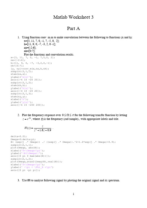
Matlab Worksheet 3Part A1. Using function conv_m.m to make convolution between the following to functions (x and h):x=[3, 11, 7, 0, -1, 7, -5, 0, 2]; h=[11, 9, 0, -7, -3, 2, 0 -1]; nx=[-2:6]; nh=[0:7];Plot the functions and convolution results.x=[3, 11, 7, 0, -1, 7,5,0, 2]; nx=[-2:6];h=[11, 9, 0, -7, -3,2,0,-1]; nh=[0:7];[y, ny]=conv_m(x,nx,h,nh); subplot(3,1,1); stem(nx,x); ylabel('x[n]');axis([-6 10 -20 20]); subplot(3,1,2); stem(nh,h); ylabel('h[n]');axis([-4 10 -20 20]); subplot(3,1,3); stem(ny,y); xlabel('n'); ylabel('y[n]');axis([-6 15 -200 200]);2. Plot the frequency response over π≤Ω≤0for the following transfer function by lettingΩ=j e z , where Ωis the frequency (rad/sample)., with appropriate labels and title.9.06.1)(2++=z z zz H .delta=0.01;Omega=0:delta:pi;H= (exp(j .* Omega)) ./ ((exp(j .* Omega)).^2+1.6*exp(j .* Omega)+0.9); subplot(2,1,1);plot(Omega, abs(H)); xlabel('0<\Omega<\pi'); ylabel('|H(\Omega)|');axis([0 pi 0 max(abs(H))]); subplot(2,1,2);plot(Omega,atan2(imag(H),real(H))); xlabel('0<\Omega<\pi');ylabel(' -\pi < \Phi_H <\pi') axis([0 pi -pi pi]);3. Use fft to analyse following signal by plotting the original signal and its spectrum.⎪⎭⎫ ⎝⎛+⎪⎭⎫ ⎝⎛+⎪⎭⎫ ⎝⎛=10244672sin 10241372sin 1024322sin ][n n n n x πππ.% fft N=1024; dt=1/N;t=0:dt:1-dt;x=sin(2*pi*32 .*t) +sin(2*pi*137 .*t)+sin(2*pi*467 .*t) ; subplot(2,1,1);plot(t,x), xlabel('t sec'),ylabel('x'); title('Signal and its Fourier Transform'); axis([min(t) max(t) 1.5*min(x) 1.5*max(x)]); X=fft(x); f=0:N-1;subplot(2,1,2);stem(f,abs(X)), xlabel('Hz'), ylabel('|X|'); axis([ 0 N/2 0 1.5*max(abs(X))]);4. Use the fast Fourier transform function fft to analyse following signal. Plot the original signal,and the magnitude of its spectrum linearly and logarithmically. Apply Hamming window to reduce the leakage.⎪⎭⎫ ⎝⎛+⎪⎭⎫ ⎝⎛+⎪⎭⎫ ⎝⎛=10247.4672sin 10244.1372sin 10245.322sin ][n n n n x πππ.The hamming window can be coded in Matlab asfor n=1:Nhamming(n)=0.54+0.46*cos((2*n-N+1)*pi/N); end;where N is the data length in the FFT.%Examine signal components %sampling rate 1024Hz N=1024; dt=1/N;t=0:dt:1-dt;%****define the signal**x=0.1*sin(2*pi*32.5 .*t ) + ... 0.2*sin(2*pi*137.4 .*t )+ ... 0.15*sin(2*pi* 467.7 .*t ) ; %*********************** subplot(3,1,1); plot(t,x);axis([0 1 -1 1]);xlabel('nT (seconds)'); ylabel('x[n]');%hamming window for n=1:Nw(n)=0.54+0.46*cos((2*n-N+1)*pi/N); end ;x1=x .*w;subplot(3,1,2); plot(t,x1);axis([0 1 -5 5]);xlabel('nT (seconds)'); ylabel('x[n] Hamming win'); X=fft(x1);df=1;f=0:df:N-1;subplot(3,1,3);plot(f,20*log10(abs(X))); axis([0 N/2 -60 60]);xlabel('k (Hz)');ylabel('|X[k]| (db)');Part BSimulation Using SIMULINKINTRODUCTIONThe objective of this laboratory is to learn about various properties of signals and systems by doing simulations in SIMULINK.PART 1. BASICS OF SIMULINK1.1 UNDERSTANDING SIMPLE WAVEFORMS AND INTEGRATIONCreate a pulse of height 2 units from time 0 to 4 seconds by subtracting two unit steps and adding a gain. Connect this pulse to an integrator with a gain of 0.5 and a zero initial condition. Connect oscilloscopes to show the pulse and the output of the integrator. You may wish to name your simulation (block) diagram; to do so use the save as feature under edit. Your block diagram should be similar as below.Before simulating you need to pull down the simulation header and double click on parameters. Unless told otherwise always assume that you can use the ode 45 integration algorithm shown in this window and the other default parameters. Typically you will only alter the start and stop times but for this first simulation you can use the default values of 0 and 10 seconds. Double click on the oscilloscopes to get the windows in which the traces will appear, pull down the simulate menu and click on run. Plot below the integrator input and output waveforms.Repeat the experiment but with an initial condition of –2 on the integrator. Again draw the results.Repeat the experiment but with an initial condition of –2 on the integrator. Again draw the results.1.2 FIRST ORDER SYSTEMA single time constant may be simulated using the transfer function block in which you enter the coefficients of the numerator and denominator polynomials. Set up the configuration in a new SIMULINK window to realise the transfer function 1/(s+2) with the input unit step and an oscilloscope connected to the output of the transfer function block. Plot the block diagram in the space below. Simulate the system for 5 seconds and plot the response.1.3 SECOND ORDER SYSTEMFor the second order all pole transfer function )2/(200220ωωζω++s s you will recall that if a time scale of ω0t is used for plotting the step response, the response shape will only be affected by changes in the damping ratio ζ. This can also be shown if we normalise the transfer function by replacing (s/ω0) by s n togive )12/(12++n n s s ζ. To study the effect of varying ζ on the step response we will therefore use the transfer function 1/(s 2+2ζs+1). Set up the following configuration for a simulation study.i) A unit step input. ii) Connect the unit step to a transfer function of 1/(s 2+2ζs+1) with ζ = 1.0. iii) Take a summing block and connect the input step to a +ve input and the transfer functionoutput to a –ve input.iv) Connect the output of this summer to a square function. This is obtained by using f(u) in thenonlinear blocks.v)Connect the output of this squarer to an integrator.vi)Connect two oscilloscopes to the circuit, one to the transfer function output and the other to the output of the integrator.vii)Also connect simout blocks to the same signals as the oscilloscopes. Rename the one connected to the integrator output simout1.Simulate the system with the values of ζ listed in the table below and fill in the other figures from the simulation results. To get an accurate value at the end of each run you can type simout1 in the MATLAB window. You can also measure the overshoot by making use of the maximum command: simply type max(simout) in the MATLAB window.% overshoot 2.1076 1.2500 1.1778 1.0571 1.0000 1.1285 2.1431PART 2. SIMULATION OF AIRCRAFT PITCH ANGLE AND ALTITUTEThe purpose IS to use "SIMULINK" to simulate a (much simplified) model of the longitudinal motion of a fighter aircraft.The "angle of attack", is the angle between the direction a plane is pointing, and the direction in which it actually moves through the air. For a plane flying at approximately constant altitude, this is equivalent to the "pitch angle", φ, as illustrated in Fig.2.1. This angle is important because it produces a lift force perpendicular to the axis of the plane, and hence a "normal acceleration", a n , (also shown in the figure).vThe pilot wants to be able to control the pitch angle (倾斜角度), and does so ultimately by rotating the front fins, and tail elevators of the aircraft, shown in Fig. 2.2. The first task is therefore to model theeffect of these movements on the "pitch rate" q ()=φ, and "normal acceleration" a n .Fig. 2.2 Illustration of control surfaces2.1: MODELLING THE AIRCRAFT AND ACTUATOR DYNAMICSi) Normal Acceleration, a nThe acceleration of the aircraft in a direction perpendicular to its axis, (the "normal accel.", a n ), is determined mainly by the angle θ1 of the tail elevators of the aircraft shown in Fig. 2.2. Indeed aerodynamic modelling shows that this relationship can be described by the differential equation,11116342.364.1982.81.3θθθ++=-+ n n n a a aConvert this relationship into a transfer function form:-ii) Pitch Rate, qThe rate at which the pitch angle changes, (the "pitch rate", q ), is determined mainly by the angle θ2 of the front fins of the aircraft shown in Fig. 2.2. Indeed aerodynamic modelling shows that this relationship can be described by the differential equation,2227.1125.782.81.3θθ++=-+ q q qConvert this relationship into a transfer function form:-iii) Actuator Dynamics + GearsThe tail elevators of the aircraft are driven directly by a hydraulic actuator which has a transfer function,G s s ()()=-+1414/ (3)To a unit step input U(s)=1/s , the response R(s) = G(s)⋅U(s)= 1411)14(14++-=+-s s s s . What form ofstep response r(t) would you expect from this actuator, and what is its time constant?The front fins and the tail elevators are both driven from the actuator by the same drive shaft through a gear box. The same gear on this drive shaft connects to the tail elevator gear wheel, which has 500 teeth, and the front fin gear wheel, which has 100 teeth, the relationship between θ1 and θ2 is52112==t t θθ(4) 2.2: SIMULATING THE AIRCRAFT AND ACTUATOR DYNAMICSi) F or the aircraft model you will need from the Continuous or Maths Library:-∙a Transfer Fcn block to represent the "tail elevator angle → normal accel" relationship (eqn (1))∙ a Transfer Fcn block to represent "front fin angle → pitch rate" relationship, (see eqn (2)) ∙ a Transfer Fcn block to represent the hydraulic "actuator dynamics", (see eqn (3)) ∙ a Gain block to represent the "gears", (see eqn (4))from the Sources Library:-∙ a Step Input block to act as a test input - (set Step time = 5sec, and Final value = 0.01 rad)from the Sinks Library:- ∙a ‘Scope block to monitor the pitch rate output - (set Horizontal Range = 20sec).ii) Now connect the blocks together, using the step input to drive the actuator, and the actuator to drive the tail elevators. The actuator is also used to drive the front fins via the gearbox. The 'Scope should be connected to the output of the "front fin angle → pitch rate" block. Note: you can take a branch from a signal line by dragging with the right mouse button from the point on the line at which you want the branch to start.Plot the block diagram you have created in the box below:-iii) From the pull-down menus of your simulation window, select Simulation/Parameters , in order to define how the simulation is to be performed. Set:-Stop Time = 20 sec; Initial Step Size = 0.001; Max Step Size = 0.01;iv) Finally double click on your ‘scope, so that you can watch the progress of the simulation, and then select Simulation/Start from the pull-down menu of your simulation window. You may want to adjustthe Vertical Range of your 'Scope, and re-run the simulation to get a good picture. Plot the response of the aircraft pitch rate below, and comment on these results. Note that it can be shown that if a transfer function has a denominator polynomial with a zero or negative coefficient then it must have a root with a zero or positive real part.2.3: SIMULATING THE PITCH RATE CONTROL SYSTEMThe designers are quite glad they simulated the response of the aircraft, before trying it for real. They now decide to improve the response by measuring the output (ie. what is actually happening to the pitch rate), and subtracting this from the input (ie. what they would like to happen), to produce an error signal. The error signal will be amplified, and then used to drive the actuator (see Fig. 2.3). In this way the actuator will automatically act so as to reduce any differences between the input demand, and the output response.Fig. 2.3 Feedback control of pitch ratei) Before you simulate the control system described above, you will probably find that you are short of space in your simulation window. Besides it would be nice to package the aircraft + actuator dynamics as a single block, so that they are distinct from anything added later as shown in Fig. 2.3.If you press the left mouse button in an empty space of the window, you get a "rubber band" box which you can drag to surround a group of elements. When you release the button, all elements inside are "selected". Use this technique to select all the aircraft + actuator dynamics, (but leave out the step input and ‘scope monitor). From the pull-down menu under Edit select Create a Subsystem, and your diagram will suddenly look as shown in Fig. 2.4.Fig. 2.4 New diagramii) Rename the "Subsystem" as "Actuator + Aircraft Dynamics" as shown in Fig. 2.3 by editing the text below the block. You can see what is inside by double clicking on the block itself, - try it! Notice that the input and output connections are labelled "in_1", "out_1" etc. Edit these to give them more meaningful names.iii) Now construct the planned control system, as illustrated in Fig. 2.3. Notice the pilot is now represented by a Signal Generator (from the Sources library), which should be set to produce a Square Wave, of frequency 0.1 Hz and peak amplitude 0.5.iv) The designers are unsure what value to use for the Gain. Open the Pitch Rate 'Scope, and run the simulation first for the Gain = -0.5 (as shown above), and then for the Gain = -5. Plot the two responses you obtain, and comment on the relative advantages and disadvantages of each:-Comments on responses (in terms of overshot and response time etc):PART 3: SIMILATION OF NONLINEAR SHIP ROLL DYNAMICSThe rolling motion of ships is of considerable interest to naval architects because even today around 50% of ships lost at sea, sink as a result of a capsize. The aim of this laboratory is to study such behaviour by:-∙constructing a nonlinear differential equation model for the system∙converting this model into a phase variable block diagram form suitable for simulation∙simulating the (nonlinear) response to sinusoidal excitation∙calculating the steady state response for a ship whose cargo has shifted dangerously to one sideFig. 3.1 Ship schematic3.1: MODELLING AND SIMULATION OF SHIP DYNAMICSi) Consider the ship sketch shown in Fig. 3.1. Given that:-∙ The effective inertia of the ship about its roll axis = J (1) ∙ The damping moment / torque due to friction between the body of the ship and the water, and due to turbulence round the "bilge keels" = c c 123 θθ+ (2) ∙ The restoring moment / torque due to the buoyancy and shape of the ship, as it is pushed to oneside = k k k 12335θθθ++ (3) ∙ The input / forcing moment due to the wave forces acting on the ship = u t ()- Using Newton’s second law of motion ∑=Torque Moment J / θ , the nonlinear differential equation which describes the rolling motion of the ship can be written as:-()()53321321)(θθθθθθk k k c c t u J ++-+-= (4)(ii) Re-arrange equation (4) to obtain an expression for the highest derivative of the output signal θ:-()()()53321321)(1θθθθθθk k k c c t u J++-+-= (5)iii) Hence complete the drawing of the SIMULINK block diagram for the ship roll system:-3.2: SIMULATING THE SHIP DYNAMICSi) For the ship model you will need:-from the Continuous and Maths Library:-∙ a few Integrator blocks - (assume zero initial conditions for now)∙ a few Gain blocks (not absolutely necessary)from the Nonlinear Library:-∙ a couple of Fcn blocks to implement the damping and stiffness terms (eqns (2), and (3)) from the Sources Library:- ∙ a Sine Wave block to simulate the sea waves u(t) - (set Ampl = 0.3 , and Freq = 0.6 rad/s)from the Sinks Library:-∙ a To Workspace block for the output ship roll angle, θ, of the simulation. This stores the results in a MATLAB variable which we can plot later, -(set the Variable name = theta, and the Maximum number of timesteps (ie points stored) = 5000)∙ an oscilloscope if you wish to see a waveform whilst the simulation is taking placeii) Drag the appropriate blocks over into your simulation window using the mouse, and double click on them to enter the appropriate parameter values. The numerical values for the coefficients of eqn (4) are:-;150;20;8.0;8.0;02.0;132121======k k k c c J(6)Note these values are given in consistent units so that θ is in radians. Finally by clicking on the text under each block, you can also enter a suitable description for each.iii) Now connect the blocks together, according to the phase variable block diagram you have plotted in section A. Note that some blocks will need changing so they "face the other way"; you can do this by selecting the block and "Flipping Horizontally " using the Options pulldown menu. Remember too that you can take a branch from a signal line by dragging with the right mouse button from the point on the line at which you want the branch to start.iv) From the pull-down menus of your simulation window, select Simulation/Parameters , in order to define how the simulation is to be performed. Set:-Stop Time = 10*pi (sec); Initial Step Size = 0.001; Max Step Size = 0.1;v) Now run the simulation by selecting Simulation/Start from the pull-down menu of your simulation window. If you do not use an oscilloscope you probably won't see much happening because the results are being stored in the MATLAB variable called 'theta', instead of being displayed immediately. After a few seconds however, you should hear a slight beep indicating the simulation is complete. Use of an oscilloscope is, however, recommended so that you can see if things ‘look all right’.vi)Now plot your results by typing plot(theta)at the MATLAB prompt in the MATLAB command window. Plot the response below, and comment on how it differs from what you would expect from a linear system if this were also excited with a sine wave input.。
物理光学作业参考答案[13-1] 波长nm 500=λ的单色光垂直入射到边长3cm 的方孔,在光轴(它通过孔中心并垂直孔平面)附近离孔z 处观察衍射,试求出夫琅和费衍射区的大致范围。
解:夫琅和费衍射条件为:π<<+zy x k2)(max2121 即: m nm y x z 900109.0500)1015()1015()(122626max2121=⨯=⨯+⨯=+>>λ[13-3]平行光斜入射到单缝上,证明:(1)单缝夫琅和费衍射强度公式为20)sin (sin )]sin (sin sin[⎪⎪⎭⎪⎪⎬⎫⎪⎪⎩⎪⎪⎨⎧--=i a i a I I θλπθλπ 式中,0I 是中央亮纹中心强度;a 是缝宽;θ是衍射角,i 是入射角(见图)。
证明:(1缝上任意点Q 的位矢:单逢上光场的复振幅为:因此,观察面上的夫琅和费衍射场为: (其中: ))cos ,0,(sin i i k k =)0,,(11y x r = 1sin 1)(~x i ik rk i Ae Ae x E ⋅⋅== )sin (sin )]sin (sin sin[)(~1)(~)2(1122)sin (sin )2(11sin 22sin )2(11221)2(11211211112111121i a i a ae z A dx e e z i A dx e e e z i A dx e x E e z i x E z x z ik a a x i ik z x z ik x ik a a x i ik z x z ik x z x ik a az x z ik --====+---+⋅--⋅+--+⎰⎰⎰θλπθλπλλλλθθθsin 1≈z x所以,观察面上的光强分布为:式中:(2)第一暗点位置:[13-4]在不透明细丝的夫琅和费衍射图样中,测得暗条纹的间距为1.5mm ,所用透镜的焦距为30mm ,光波波长为632.8nm 。
1.工程光学系列之一:杨氏双缝干涉matlab1.基本原理杨氏干涉实验是两点光源干涉实验的典型代表。
杨氏干涉实验以极简单的装置和巧妙构思实现了普通光源干涉。
无论从经典光学还是从现代光学的角度来看,杨氏实验都具有十分重要的意义。
杨氏双缝实验的装置如图2-18所示,按照惠更斯-菲涅耳原理,线光源S上的点将作为次波源向前发射次波(球面波),形成交叠的波场。
在较远的地方放置一观察屏,屏上可以观测到一组几乎是平行的直线条纹。
图杨氏干涉实验原理图2.matlab源代码clearlam=500e-9;a=2e-3;D=1;ym=5*lam*D/a;xs=ym;n=101;ys=linspace(-ym,ym,n);for i=1:nr1=sqrt((ys(i)-a/2).^2+D^2); r2=sqrt((ys(i)+a/2).^2+D^2); phi=2*pi*(r2-r1)./lam;B(i,:)=sum(4*cos(phi/2).^2); endN=255;Br=(B/4.0)*N;subplot(1,2,1)image(xs,ys,Br); colormap(gray(N)); subplot(1,2,2)plot(B,ys)3.实验现象2. 工程光学系列之二:等倾干涉matlab2.1 基本原理等倾干涉是薄膜干涉的一种。
薄膜此时是均匀的,光线以倾角i入射,上下两条反射光线经过透镜作用会汇聚一起,形成干涉。
化学教案权倾一时化学教案内外无不造门者化学教案唯景仁不至试卷试题年三十化学教案方为著作佐郎试卷试题桓玄诛元图等倾干涉薄膜由于入射角相同的光经薄膜两表面反射形成的反射光在相遇点有相同的光程差,也就是说,凡入射角相同的就形成同一条纹,故这些倾斜度不同的光束经薄膜反射所形成的干涉花样是一些明暗相间的同心圆环.这种干涉称为等倾干涉。
倾角i相同时,干涉情况一样(因此叫做“等倾干涉”)2.2 matlab源代码%等倾干涉clear allclose allclc%%k=2000;s=500;D=0.2;bochang=s*10^(-9);theta=0.15;d=k*bochang/4;rMax=D*tan(theta/2);N=501;for i=1:Nx(i)=(i-1)*2*rMax/(N-1)-rMax; for j=1:Ny(j)=(j-1)*2*rMax/(N-1)-rMax; r(i,j)=sqrt(x(i)^2+y(j)^2);delta(i,j)=2*d/sqrt(1+r(i,j)^2/D^2); Phi(i,j)=2*pi*delta(i,j)/bochang; B(i,j)=4*cos(Phi(i,j)/2)^2;endendNCLevels=255;Br=(B/4.0)*NCLevels;figure(1);image(x,y,Br);colormap(gray(NCLevels));2.3 实验现象3. 工程光学系列之三:夫琅禾费矩孔衍射matlab3.1 实验原理衍射的定义:光波在传播过程遇到障碍物时,光束偏离直线传播,强度发生重新分布的现象。
光的干涉和衍射一、实验目的① 学习用用模拟实验方法探究光的干涉和衍射问题.② 进一步熟悉MA TLAB 编程.二、实验内容和要求1. 双缝干涉模拟实验杨氏双缝干涉实验是利用分波前法获得相干光束的典型例子. 如图2.24所示,单色光通过两个窄缝s 1,s 2射向屏幕,相当于位置不同的两个同频率同相位光源向屏幕照射的叠合,由于到达屏幕各点的距离(光程)不同引起相位差,叠合的结果是在有的点加强,在有的点抵消,造成干涉现象.图2.24 双缝干涉示意图 考虑两个相干光源到屏幕上任意点P 的距离差为1221r r r r r ==∆=- (2.19) 引起的相位差为2πrϕλ∆=设两束相干光在屏幕上P 点产生的幅度相同,均为A 0,则夹角为φ的两个矢量A 0的合成矢量的幅度为A =2A 0 cos(φ/2)第二章 数理探究试验 135光强B 正比于振幅的平方,故P 点光强为B =4B 0cos 2(φ/2) (2.20)运行sy211.m 程序得到干涉条纹如图2.27所示.clear all %sy211.mlam=500e-9; %输入波长a=2e-3; D=1;ym=5*lam*D/a; xs=ym; %设定光屏的范围n=101;ys=linspace(-ym,ym,n); % 把光屏的y 方向分成101点for i=1:nr1=sqrt((ys(i)-a/2).^2+D^2);r2=sqrt((ys(i)+a/2).^2+D^2);phi=2*pi*(r2-r1)/lam;B(i,:)=4*cos(phi/2).^2;endN=255; % 确定用的灰度等级为255级Br=(B/4.0)*N; %使最大光强对应于最大灰度级(白色)subplot(1,2,1)image(xs,ys,Br); %画干涉条纹colormap(gray(N));subplot(1,2,2)plot(B,ys) %画出光强变化曲线图2.25中左图是光屏上的干涉条纹,右图是光屏上沿y 轴方向光强的变化曲线. 从图中也不难看出,干涉条纹是以点o 所对应的水平线为对称,沿上下两侧交替,等距离排列,相邻亮条纹中心间距为2.5×10⁻⁴m. -0.4-0.200.20.4-1.5-1-0.500.511.5x 10图2.25 单色光的干涉条纹这与理论推导和实验结果基本一致.下面我们从理论上加以推导,由上面的式(2.19)可得22212121()()2d r r r r r r y -=+-=-1.5 -1 -0.5 0 0.5 1 1.5 -0.4 -0.2 0 0.4 0.2基于MA TLAB 的数学实验136 考虑到a ,y 很小,(r 1+r 2)=2D ,所以21D r r y a-= 这样就得到点P 处于亮条纹中心的条件为20122D y k k a λ==±±,,,, (2.21) 因此,亮条纹是等间距的,相邻条纹间距为94150010 2.510m 0.002D a λ--=⨯=⨯. 问题2.39:推导出点P 处于暗条纹中心的条件并与模拟结果相比较,看是否一致? 考虑到纯粹的单色光不易获得,通常都有一定的光谱宽度,这种光的非单色性对光的干涉会产生何种效应,下面我们用MA TLAB 计算并仿真这一问题.非单色光的波长不是常数,必须对不同波长的光分别处理再叠加起来. 我们假定光源的光谱宽度为中心波长的±10%,并且在该区域均匀分布. 近似取11根谱线,相位差的计算表达式求出的将是不同谱线的11个不同相位. 计算光强时应把这11根谱线产生的光强叠加并取平均值,即211012π4cos ()211k kk k r B B ϕλϕ=∆==∑ 将程序sy211.m 中的9,10两句换成以下4句,由此构成的程序就可仿真非单色光的干涉问题. N1=11;dL=linspace(-0.1,0.1,N1);%设光谱相对宽度±10%, lam1=lam*(1+dL');%分11根谱线,波长为一个数组 Phi1=2*pi*(r2-r1)./ lam1;%从距离差计算各波长的相位差 B(i, :)=sum(4*cos(Phi1/2).^2)/N1; %叠加各波长并影响计算光强运行修改后的程序得到的干涉条纹如图2.26所示. 可以看出,光的非单色性导致干涉现象的减弱,光谱很宽的光将不能形成干涉.第二章 数理探究试验 137-0.4-0.200.20.4-1.5-1-0.500.511.5-3-3图2.26 非单色光的干涉条纹 2. 单缝衍射的模拟实验一束单色平行光通过宽度可调的狭缝,射到其后的光屏上. 当缝宽足够小时,光屏上形成一系列亮暗相间的条纹,这是由于从同一个波前上发出的子波产生干涉的结果. 当光源到衍射屏的距离和光屏到衍射屏的距离都是无穷大时,即满足远场条件时,我们称这种衍射为夫琅禾费衍射. 所以夫琅禾费衍射中入射光和衍射光都是平行光. 为了模拟单缝衍射现象,我们把单缝看成一排等间隔光源,共NP 个光源分布在A ~B 区间内,离A 点间距为yp ,则屏幕上任一点S 处的光强为NP 个光源照射结果的合成.如图2.27所示,子波射线与入射方向的夹角ϕ称为衍射角,0=ϕ时,子波射线通过透镜后,必汇聚到O 点,这个亮条纹对应的光强称为主极大. NP 个光源在其他方向的射线到达S 点的光程差,应等于它们到达平面AC 的光程差,即sin yp ϕ∆=,其中sin ys Dϕ≈ ys 为S 点的纵坐标,则与A 点光源位相差为2π2πyP ys Dαλλ=∆=s O基于MA TLAB 的数学实验 138 -0.4-0.200.20.4-1.5-1-0.500.511.5-3-3图2.28 单缝衍射条纹图2.27 单缝衍射的模拟实验设单缝上NP 个光源的振幅都为1,在x ,y 轴上的分量各为cos sin αα,,合振幅的平方为:()()22COSa COSa ∑+∑. 又光强正比于振幅的平方,所以相对于O 点主极大光强也为22(cos )(sin )0I I αα=+∑∑程序sy212.m 模拟了单缝衍射现象,这里取波长λ=500nm ,缝宽a =1mm ,透镜焦距D =1m ,运行结果如图2.28所示.clear all %sy212.mlam=500e-9;a=1e-3;D=1;ymax=3*lam*D/a; %屏幕范围(沿y 向)Ny=51; %屏幕上的点数(沿y 向)ys=linspace(-ymax,ymax,Ny);NP=51;yP=linspace(0,a,NP); %把单缝分成NP 个光源for i=1:Ny %对屏幕上y 向各点作循环SinPhi=ys(i)/D;alpha=2*pi*yP*SinPhi/lam; SumCos=sum(cos(alpha)); SumSin=sum(sin(alpha));B(i,:)=(SumCos^2+SumSin^2)/NP^2;end N=255; % 确定用的灰度等级为255级%使最大光强对应于最大灰度级(白色)Br=B/max(B)*N; subplot(1,2,1)%画衍射条纹,用灰度级颜色图image(ymax,ys,Br); colormap(gray(N));subplot(1,2,2)%画屏幕上光强曲线 plot(B,ys,'*',B,ys);grid;分析图2.28中的衍射条纹,我们可以看出所有亮暗条纹都平行于单缝,O 点光强为最大,这都和理论推导结果相一致.问题2.40: 从理论上讲,中央亮条纹的半角宽和第一条暗条纹的衍射角都应等于λ/a ,各次极大角宽都等于中央亮条纹的半角宽,图2.28模拟的衍射条纹符合这个结论吗?3. 光栅衍射的模拟实验有大量等宽度、等间距的平行狭缝组成的光学系统称为衍射光栅. 单缝宽度a 和刻第二章 数理探究试验 139痕宽度b 之和称为光栅常数d ,d =a +b . 光栅衍射条纹是单缝衍射和缝间干涉的共同结果.设光栅有N 条狭缝,透镜焦距为D ,理论分析可以得到,光屏上P 点的夫琅禾费衍射光强I P /I 0分布为220sin sin ()()sin P I N I αβαβ= 式中sin sin sin s y a d Dππαϕβϕϕλλ==≈,, 运行程序sy213.m 得到衍射条纹如图2.29所示.clear all %sy213.mlam=632.8e-9; N=2;a=2e-4; D=5;d=5*a;ym=1.89*lam*D/a;xs=ym; %设定光屏的范围n=1001;ys=linspace(-ym,ym,n); % y 方向分成1001点for i=1:nSinphi=ys(i)/D;alpha=pi*a*Sinphi/lam;beta=pi*d*Sinphi/lam;B(i, :)=(sin(alpha)./alpha).^2.*(sin(N*beta)./sin(beta)).^2 ;B1=B/max(B); %将最大光强设为1endNC=255;Br=B/max(B)*NC;subplot(1,2,1)image(xs,ys,Br); %画衍射条纹colormap(gray(NC))subplot(1,2,2)plot(B1,ys) %画出沿y 向的相对光强变化曲线问题2.41:程序sy213.m 中d =5a ,观察图2.29衍射条纹,看有无缺级现象,为什么?改变sy213.m 中的波长、缝宽、光栅常数值,看衍射条纹有何变化?试加以解释.基于MA TLAB 的数学实验 140-0.4-0.200.20.4-0.025-0.02-0.015-0.01-0.0050.0050.010.0150.020.025图2.29 光栅衍射条纹第二章数理探究试验141 《车辆制冷与空调》第二次作业参考答案《车辆隔热壁》、《制冷方法与制冷剂》、《蒸汽压缩式制冷》一.简答题1.什么是隔热壁的传热系数?它的意义是什么?答:隔热壁的传热系数指车内外空气温度相差1℃时,在一小时内,通过一平方米热壁表面积所传递的热量。
matlab作业3参考答案Matlab作业3参考答案Matlab作业3是一个综合性的编程任务,要求学生运用Matlab的各种功能和工具来解决实际问题。
本文将提供Matlab作业3的参考答案,并对其中的关键步骤和思路进行详细解释。
一、问题描述在本次作业中,学生需要解决一个关于图像处理的问题。
具体来说,给定一张彩色图像,学生需要编写Matlab代码来实现以下功能:1. 将彩色图像转换为灰度图像;2. 对灰度图像进行高斯滤波;3. 对滤波后的图像进行边缘检测;4. 对边缘图像进行二值化处理。
二、解决方案1. 将彩色图像转换为灰度图像首先,我们需要读取彩色图像。
可以使用Matlab的imread函数来实现。
然后,使用rgb2gray函数将彩色图像转换为灰度图像。
代码如下:```matlabrgbImage = imread('image.jpg');grayImage = rgb2gray(rgbImage);```2. 对灰度图像进行高斯滤波接下来,我们需要对灰度图像进行高斯滤波。
高斯滤波是一种常用的图像平滑方法,可以有效地去除图像中的噪声。
Matlab提供了fspecial函数来生成高斯滤波器。
代码如下:```matlabh = fspecial('gaussian', [3 3], 1);filteredImage = imfilter(grayImage, h);```3. 对滤波后的图像进行边缘检测在这一步中,我们需要对滤波后的图像进行边缘检测。
边缘检测可以帮助我们找到图像中的边缘和轮廓。
Matlab提供了多种边缘检测算法,如Sobel算子和Canny算子。
代码如下:```matlabedgeImage = edge(filteredImage, 'canny');```4. 对边缘图像进行二值化处理最后,我们需要对边缘图像进行二值化处理,将图像中的边缘转换为黑白两种颜色。
物理光学作业3-2
波的叠加原理+ 数值仿真
使用Matlab 仿真两个相干光束在观察屏上的干涉条纹,一个光束是与光轴成θ角的平面波,另一个光束是点光源发出的球面波,由于L>>λ,在观察屏上该球面波可以采用旁轴近似。
其中相关参数如下:θ=0,0.0001,0.0004,0.0008 时, L=2m, 观察屏D=0.01m, 振幅A=1,
λ=1μm
通过给定条件,完成如下要求:
1 建立观察屏上的任意点P 的光强表达式I(x,y);
2 画出观察屏上的条纹图样。
3 分析各种不同θ角度时干涉条纹的形状。
图1
一:建立数学模型
平面波与球面波进行叠加,如图1所示,P点的光强I=I1+I2+2√I1I2COSδ,δ=2πD/λ=2π(r1-r2)/λ,D为光程差。
设P 点为(x,y),则:
r1=√(x^2+y^2+l^2)
r2=l/cos(θ)-l*sin(θ)*tan(θ)+x*sin(θ)
I=4cos^2(πD/λ)
二:仿真
MATLAB代码如下:
L=200;
lamda=10^-4;
theta=input('theta=');
xmax=0.5;
ymax=xmax;
y=linspace(-ymax,ymax,5000);
x=linspace(-xmax,xmax,5000);
for i=1:5000
for j=1:5000
r1=sqrt(x(i)^2+y(j)^2+L^2);
r2=L/cos(theta)+y(j)*sin(theta)-
L*sin(theta)*tan(theta);
D=r1-r2;
phi=2*pi*D/lamda;
I0(i,j)=4*cos(phi/2)^2;
end
end
I=(I0/4)*255
colormap(gray(255));
image(x,y,I);
当θ=0时,得到的干涉条纹如图 2
图2
当θ=0.0001时,得到的干涉条纹如图3所示
图3
当θ=0.0004时,得到的干涉条纹如图4
图4
当θ=0.0008时,得到的干涉条纹如图5
图5
三:结果分析
观察不同角度的平行光与球面光的干涉图像,可以看出,随着平行光角度的变化,干涉的同心圆条纹中心也在移动。
这是因为,随着平行光的角度变化,相对应的光程也发生变化,与球面光的光程差为零的点发生移动,即圆心发生偏移。
四:总结与感悟
在这次的电子作业中,用Matlab软件来进行光的干涉的仿真,建立直观的物理图像,加深对光学现象的认识,培养独立思考的能力。
通过这次作业,我更好的理解干涉条纹间距与L、d、间的关系,更加明白干涉的实质,为以后的学习有很大帮助。