Realization of PID controls by fuzzy control methods

目录Part 1 PID type fuzzy controller and parameters adaptive method (1)Part 2 Application of self adaptation fuzzy-PID control for main steam temperature control system in power station (7)Part 3 Neuro-fuzzy generalized predictive control of boiler steam temperature ..................................................................... (13)Part 4 为Part3译文：锅炉蒸汽温度模糊神经网络的广义预测控制21Part 1 PID type fuzzy controller and Parametersadaptive methodWu zhi QIAO, Masaharu MizumotoAbstract: The authors of this paper try to analyze the dynamic behavior of the product-sum crisp type fuzzy controller, revealing that this type of fuzzy controller behaves approximately like a PD controller that may yield steady-state error for the control system. By relating to the conventional PID control theory, we propose a new fuzzy controller structure, namely PID type fuzzy controller which retains the characteristics similar to the conventional PID controller. In order to improve further the performance of the fuzzy controller, we work out a method to tune the parameters of the PID type fuzzy controller on line, producing a parameter adaptive fuzzy controller. Simulation experiments are made to demonstrate the fine performance of these novel fuzzy controller structures.Keywords: Fuzzy controller; PID control; Adaptive control1. IntroductionAmong various inference methods used in the fuzzy controller found in literatures , the most widely used ones in practice are the Mamdani method proposed by Mamdani and his associates who adopted the Min-max compositional rule of inference based on an interpretation of a control rule as a conjunction of the antecedent and consequent, and the product-sum method proposed by Mizumoto who suggested to introduce the product and arithmetic mean aggregation operators to replace the logical AND (minimum) and OR (maximum) calculations in the Min-max compositional rule of inference.In the algorithm of a fuzzy controller, the fuzzy function calculation is also a complicated and time consuming task. Tagagi and Sugeno proposed a crisp type model in which the consequent parts of the fuzzy control rules are crisp functional representation or crisp real numbers in the simplified case instead of fuzzy sets . With this model of crisp real number output, the fuzzy set of the inference consequence willbe a discrete fuzzy set with a finite number of points, this can greatly simplify the fuzzy function algorithm.Both the Min-max method and the product-sum method are often applied with the crisp output model in a mixed manner. Especially the mixed product-sum crisp model has a fine performance and the simplest algorithm that is very easy to be implemented in hardware system and converted into a fuzzy neural network model. In this paper, we will take account of the product-sum crisp type fuzzy controller.2. PID type fuzzy controller structureAs illustrated in previous sections, the PD function approximately behaves like a parameter time-varying PD controller. Since the mathematical models of most industrial process systems are of type, obviously there would exist an steady-state error if they are controlled by this kind of fuzzy controller. This characteristic has been stated in the brief review of the PID controller in the previous section.If we want to eliminate the steady-state error of the control system, we can imagine to substitute the input (the change rate of error or the derivative of error) of the fuzzy controller with the integration of error. This will result the fuzzy controller behaving like a parameter time-varying PI controller, thus the steady-state error is expelled by the integration action. However, a PI type fuzzy controller will have a slow rise time if the P parameters are chosen small, and have a large overshoot if the P or I parameters are chosen large. So there may be the time when one wants to introduce not only the integration control but the derivative control to the fuzzy control system, because the derivative control can reduce the overshoot of the system's response so as to improve the control performance. Of course this can be realized by designing a fuzzy controller with three inputs, error, the change rate of error and the integration of error. However, these methods will be hard to implement in practice because of the difficulty in constructing fuzzy control rules. Usually fuzzy control rules are constructed by summarizing the manual control experience of an operator who has been controlling the industrial process skillfully and successfully. The operator intuitively regulates the executor to control the process by watching theerror and the change rate of the error between the system's output and the set-point value. It is not the practice for the operator to observe the integration of error. Moreover, adding one input variable will greatly increase the number of control rules, the constructing of fuzzy control rules are even more difficult task and it needs more computation efforts. Hence we may want to design a fuzzy controller that possesses the fine characteristics of the PID controller by using only the error and the change rate of error as its inputs.One way is to have an integrator serially connected to the output of the fuzzy controller as shown in Fig. 1. In Fig. 1,1K and 2K are scaling factors for e and ~ respectively, and fl is the integral constant. In the proceeding text, for convenience, we did not consider the scaling factors. Here in Fig. 2, when we look at the neighborhood of NODE point in the e - ~ plane, it follows from (1) that the control input to the plant can be approximated by(1)Hence the fuzzy controller becomes a parameter time-varying PI controller, itsequivalent proportional control and integral control components are BK2D and ilK1 P respectively. We call this fuzzy controller as the PI type fuzzy controller (PI fc). We can hope that in a PI type fuzzy control system, the steady-state error becomes zero.To verify the property of the PI type fuzzy controller, we carry out some simulation experiments. Before presenting the simulation, we give a description of the simulation model. In the fuzzy control system shown in Fig. 3, the plant model is a second-order and type system with the following transfer function:)1)(1()(21++=s T s T K s G (2) Where K = 16, 1T = 1, and 2T = 0.5. In our simulation experiments, we use thediscrete simulation method, the results would be slightly different from that of a continuous system, the sampling time of the system is set to be 0.1 s. For the fuzzy controller, the fuzzy subsets of e and d are defined as shown in Fig. 4. Their coresThe fuzzy control rules are represented as Table 1. Fig. 5 demonstrates the simulation result of step response of the fuzzy control system with a Pl fc. We can see that the steady-state error of the control system becomes zero, but when the integration factor fl is small, the system's response is slow, and when it is too large, there is a high overshoot and serious oscillation. Therefore, we may want to introduce the derivative control law into the fuzzy controller to overcome the overshoot and instability. We propose a controller structure that simply connects the PD type and the PI type fuzzy controller together in parallel. We have the equivalent structure of that by connecting a PI device with the basic fuzzy controller serially as shown in Fig.6. Where ~ is the weight on PD type fuzzy controller and fi is that on PI type fuzzy controller, the larger a/fi means more emphasis on the derivative control and less emphasis on the integration control, and vice versa. It follows from (7) that the output of the fuzzy controller is(3)3. The parameter adaptive methodThus the fuzzy controller behaves like a time-varying PID controller, its equivalent proportional control, integral control and derivative control components are respectively. We call this new controller structure a PID type fuzzy controller (PID fc). Figs. 7 and 8 are the simulation results of the system's step response of such control system. The influence of ~ and fl to the system performance is illustrated. When ~ > 0 and/3 = 0, meaning that the fuzzy controller behaves like PD fc, there exist a steady-state error. When ~ = 0 and fl > 0, meaning that the fuzzy controller behaves like a PI fc, the steady-state error of the system is eliminated but there is a large overshoot and serious oscillation.When ~ > 0 and 13 > 0 the fuzzy controller becomes a PID fc, the overshoot is substantially reduced. It is possible to get a comparatively good performance by carefully choosing the value of αandβ.4. ConclusionsWe have studied the input-output behavior of the product-sum crisp type fuzzy controller, revealing that this type of fuzzy controller behaves approximately like a parameter time-varying PD controller. Therefore, the analysis and designing of a fuzzy control system can take advantage of the conventional PID control theory. According to the coventional PID control theory, we have been able to propose some improvement methods for the crisp type fuzzy controller.It has been illustrated that the PD type fuzzy controller yields a steady-state error for the type system, the PI type fuzzy controller can eliminate the steady-state error. We proposed a controller structure, that combines the features of both PD type and PI type fuzzy controller, obtaining a PID type fuzzy controller which allows the control system to have a fast rise and a small overshoot as well as a short settling time.To improve further the performance of the proposed PID type fuzzy controller, the authors designed a parameter adaptive fuzzy controller. The PID type fuzzy controller can be decomposed into the equivalent proportional control, integral control and the derivative control components. The proposed parameter adaptive fuzzy controller decreases the equivalent integral control component of the fuzzy controller gradually with the system response process time, so as to increase the damping of the system when the system is about to settle down, meanwhile keeps the proportional control component unchanged so as to guarantee quick reaction against the system's error. With the parameter adaptive fuzzy controller, the oscillation of the system is strongly restrained and the settling time is shortened considerably.We have presented the simulation results to demonstrate the fine performance of the proposed PID type fuzzy controller and the parameter adaptive fuzzy controller structure.Part 2 Application of self adaptation fuzzy-PID control for main steam temperature control system inpower stationZHI-BIN LIAbstract: In light of the large delay, strong inertia, and uncertainty characteristics of main steam temperature process, a self adaptation fuzzy-PID serial control system is presented, which not only contains the anti-disturbance performance of serial control, but also combines the good dynamic performance of fuzzy control. The simulation results show that this control system has more quickly response, better precision and stronger anti-disturbance ability．Keywords：Main steam temperature；Self adaptation；Fuzzy control；Serial control1. IntroductionThe boiler superheaters of modem thermal power station run under the condition of high temperature and high pressure, and the superheater’s temperature is highest in the steam channels．so it has important effect to the running of the whole thermal power station．If the temperature is too high, it will be probably burnt out. If the temperature is too low ,the efficiency will be reduced So the main steam temperature mast be strictly controlled near the given value．Fig l shows the boiler main steam temperature system structure.Fig.1 boiler main steam temperature systemIt can be concluded from Fig l that a good main steam temperature controlsystem not only has adequately quickly response to flue disturbance and load fluctuation, but also has strong control ability to desuperheating water disturbance. The general control scheme is serial PID control or double loop control system with derivative. But when the work condition and external disturbance change large, the performance will become instable. This paper presents a self adaptation fuzzy-PID serial control system. which not only contains the anti-disturbance performance of serial control, but also combines the good dynamic character and quickly response of fuzzy control ．1. Design of Control SystemThe general regulation adopts serial PID control system with load feed forward ．which assures that the main steam temperature is near the given value 540℃in most condition ．If parameter of PID control changeless and the work condition and external disturbance change large, the performance will become in stable ．The fuzzy control is fit for controlling non-linear and uncertain process. The general fuzzy controller takes error E and error change ratio EC as input variables ．actually it is a non-linear PD controller, so it has the good dynamic performance ．But the steady error is still in existence. In linear system theory, integral can eliminate the steady error. So if fuzzy control is combined with PI control, not only contains the anti-disturbance performance of serial control, but also has the good dynamic performance and quickly response.In order to improve fuzzy control self adaptation ability, Prof ．Long Sheng-Zhao and Wang Pei-zhuang take the located in bringing forward a new idea which can modify the control regulation online ．This regulation is:]1,0[,)1(∈-+=αααEC E UThis control regulation depends on only one parameter α.Once αis fixed ．the weight of E and EC will be fixed and the self adaptation ability will be very small ．It was improved by Prof. Li Dong-hui and the new regulation is as follow;]1,0[,,,3,)1(2,)1(1,)1(0,)1({321033221100∈±=-+±=-+±=-+=-+=ααααααααααααE EC E E EC E E EC E E EC E UBecause it is very difficult to find a self of optimum parameter, a new method is presented by Prof ．Zhou Xian-Lan, the regulation is as follow:)0(),ex p(12>--=k ke αBut this algorithm still can not eliminate the steady error ．This paper combines this algorithm with PI control ，the performance is improved ．2. Simulation of Control System3.1 Dynamic character of controlled objectPapers should be limited to 6 pages Papers longer than 6 pages will be subject to extra fees based on their length ．Fig .2 main steam temperature control system structureFig 2 shows the main steam temperature control system structure ，)(),(21s W s W δδare main controller and auxiliary controller,)(),(21s W s W o o are characters of the leading and inertia sections,)(),(21s W s W H H are measure unit.3.2 Simulation of the general serial PID control systemThe simulation of the general serial PID control system is operated by MATLAB, the simulation modal is as Fig.3.Setp1 and Setp2 are the given value disturbance and superheating water disturb & rice .PID Controller1 and PID Controller2 are main controller and auxiliary controller ．The parameter value which comes from references is as follow ：667.37,074.0,33.31)(25)(111111122===++===D I p D I p p k k k s k sk k s W k s W δδFig.3. the general PID control system simulation modal3.3 Simulation of self adaptation fuzzy-PID control system SpacingThe simulation modal is as Fig 4.Auxiliary controller is:25)(22==p k s W δ.Main controller is Fuzzy-PI structure, and the PI controller is:074.0,33.31)(11111==+=I p I p k k s k k s W δFuzzy controller is realized by S-function, and the code is as fig.5.Fig.4. the fuzzy PID control system simulation modalFig 5 the S-function code of fuzzy control3.4 Comparison of the simulationGiven the same given value disturbance and the superheating water disturbance，we compare the response of fuzzy-PID control system with PID serial control system. The simulation results are as fig.6-7.From Fig6-7,we can conclude that the self adaptation fuzzy-PID control system has the more quickly response, smaller excess and stronger anti-disturbance．4. Conclusion(1)Because it combines the advantage of PID controller and fuzzy controller, theself adaptation fuzzy-PID control system has better performance than the general PID serial control system.(2)The parameter can self adjust according to the error E value. so this kind of controller can harmonize quickly response with system stability．Part 3 Neuro-fuzzy generalized predictive controlof boiler steam temperatureXiangjie LIU, Jizhen LIU, Ping GUANAbstract: Power plants are nonlinear and uncertain complex systems. Reliable control of superheated steam temperature is necessary to ensure high efficiency and high load-following capability in the operation of modern power plant. A nonlinear generalized predictive controller based on neuro-fuzzy network (NFGPC) is proposed in this paper. The proposed nonlinear controller is applied to control the superheated steam temperature of a 200MW power plant. From the experiments on the plant and the simulation of the plant, much better performance than the traditional controller is obtained.Keywords: Neuro-fuzzy networks; Generalized predictive control; Superheated steam temperature1. IntroductionContinuous process in power plant and power station are complex systems characterized by nonlinearity, uncertainty and load disturbance. The superheater is an important part of the steam generation process in the boiler-turbine system, where steam is superheated before entering the turbine that drives the generator. Controlling superheated steam temperature is not only technically challenging, but also economically important.From Fig.1,the steam generated from the boiler drum passes through the low-temperature superheater before it enters the radiant-type platen superheater. Water is sprayed onto the steam to control the superheated steam temperature in both the low and high temperature superheaters. Proper control of the superheated steam temperature is extremely important to ensure the overall efficiency and safety of the power plant. It is undesirable that the steam temperature is too high, as it can damage the superheater and the high pressure turbine, or too low, as it will lower the efficiency of the power plant. It is also important to reduce the temperaturefluctuations inside the superheater, as it helps to minimize mechanical stress that causes micro-cracks in the unit, in order to prolong the life of the unit and to reduce maintenance costs. As the GPC is derived by minimizing these fluctuations, it is amongst the controllers that are most suitable for achieving this goal.The multivariable multi-step adaptive regulator has been applied to control the superheated steam temperature in a 150 t/h boiler, and generalized predictive control was proposed to control the steam temperature. A nonlinear long-range predictive controller based on neural networks is developed into control the main steam temperature and pressure, and the reheated steam temperature at several operating levels. The control of the main steam pressure and temperature based on a nonlinear model that consists of nonlinear static constants and linear dynamics is presented in that.Fig.1 The boiler and superheater steam generation process Fuzzy logic is capable of incorporating human experiences via the fuzzy rules. Nevertheless, the design of fuzzy logic controllers is somehow time consuming, as the fuzzy rules are often obtained by trials and errors. In contrast, neural networks not only have the ability to approximate non-linear functions with arbitrary accuracy, they can also be trained from experimental data. The neuro-fuzzy networks developed recently have the advantages of model transparency of fuzzy logic and learning capability of neural networks. The NFN is have been used to develop self-tuning control, and is therefore a useful tool for developing nonlinear predictive control. Since NFN is can be considered as a network that consists of several local re-gions, each of which contains a local linear model, nonlinear predictive control based onNFN can be devised with the network incorporating all the local generalized predictive controllers (GPC) designed using the respective local linear models. Following this approach, the nonlinear generalized predictive controllers based on the NFN, or simply, the neuro-fuzzy generalized predictive controllers (NFG-PCs)are derived here. The proposed controller is then applied to control the superheated steam temperature of the 200MW power unit. Experimental data obtained from the plant are used to train the NFN model, and from which local GPC that form part of the NFGPC is then designed. The proposed controller is tested first on the simulation of the process, before applying it to control the power plant.2. Neuro-fuzzy network modellingConsider the following general single-input single-output nonlinear dynamic system:),1(),...,(),(),...,1([)(''+-----=uy n d t u d t u n t y t y f t y ∆+--/)()](),...,1('t e n t e t e e (1)where f[.]is a smooth nonlinear function such that a Taylor series expansion exists, e(t)is a zero mean white noise and Δis the differencing operator,''',,e u y n n n and d are respectively the known orders and time delay of the system. Let the local linear model of the nonlinear system (1) at the operating point )(t o be given by the following Controlled Auto-Regressive Integrated Moving Average (CARIMA) model:)()()()()()(111t e z C t u z B z t y z A d ----+∆= (2) Where )()(),()(1111----∆=z andC z B z A z A are polynomials in 1-z , the backward shift operator. Note that the coefficients of these polynomials are a function of the operating point )(t o .The nonlinear system (1) is partitioned into several operating regions, such that each region can be approximated by a local linear model. Since NFN is a class of associative memory networks with knowledge stored locally, they can be applied to model this class of nonlinear systems. A schematic diagram of the NFN is shown in Fig.2.B-spline functions are used as the membership functions in theNFN for the following reasons. First, B-spline functions can be readily specified by the order of the basis function and the number of inner knots. Second, they are defined on a bounded support, and the output of the basis function is always positive, i.e.,],[,0)(j k j j k x x λλμ-∉=and ],[,0)(j k j j k x x λλμ-∈>.Third, the basis functions form a partition of unity, i.e.,.][,1)(min,∑∈≡j mam j k x x x x μ(3)And fourth, the output of the basis functions can be obtained by a recurrence equation.Fig. 2 neuro-fuzzy network The membership functions of the fuzzy variables derived from the fuzzy rules can be obtained by the tensor product of the univariate basis functions. As an example, consider the NFN shown in Fig.2, which consists of the following fuzzy rules: IF operating condition i (1x is positive small, ... , and n x is negative large),THEN the output is given by the local CARIMA model i:...)()(ˆ...)1(ˆ)(ˆ01+-∆+-++-=d t u b n t y a t y a t yi i a i in i i i a )(...)()(c i in i b i in n t e c t e n d t u b c b -+++--∆+ (4)or )()()()()(ˆ)(111t e z C t u z B z t yz A i i i i d i i ----+∆= (5) Where )()(),(111---z andC z B z A i i i are polynomials in the backward shift operator 1-z , and d is the dead time of the plant,)(t u i is the control, and )(t e i is a zero mean independent random variable with a variance of 2δ. The multivariate basis function )(k i x a is obtained by the tensor products of the univariate basis functions,p i x A a nk k i k i ,...,2,1,)(1==∏=μ (6)where n is the dimension of the input vector x , and p , the total number of weights in the NFN, is given by,∏=+=nk i i k R p 1)( (7)Where i k and i R are the order of the basis function and the number of inner knots respectively. The properties of the univariate B-spline basis functions described previously also apply to the multivariate basis function, which is defined on the hyper-rectangles. The output of the NFN is,∑∑∑=====p i i i p i ip i i i a y aa yy 111ˆˆˆ (8) 3. Neuro-fuzzy modelling and predictive control of superheatedsteam temperatureLet θbe the superheated steam temperature, and θμ, the flow of spray water to the high temperature superheater. The response of θcan be approximated by a second order model:The linear models, however, only a local model for the selected operating point. Since load is the unique antecedent variable, it is used to select the division between the local regions in the NFN. Based on this approach, the load is divided into five regions as shown in Fig.3,using also the experience of the operators, who regard a load of 200MW as high,180MW as medium high,160MW as medium,140MW as medium low and 120MW as low. For a sampling interval of 30s , the estimated linear local models )(1-z A used in the NFN are shown in Table 1.Fig. 3 Membership function for local modelsTable 1 Local CARIMA models in neuro-fuzzy modelCascade control scheme is widely used to control the superheated steam temperature. Feed forward control, with the steam flow and the gas temperature as inputs, can be applied to provide a faster response to large variations in these two variables. In practice, the feed forward paths are activated only when there are significant changes in these variables. The control scheme also prevents the faster dynamics of the plant, i.e., the spray water valve and the water/steam mixing, from affecting the slower dynamics of the plant, i.e., the high temperature superheater. With the global nonlinear NFN model in Table 1, the proposed NFGPC scheme is shown in Fig.4.Fig. 4 NFGPC control of superheated steam temperature with feed-for-ward control.As a further illustration, the power plant is simulated using the NFN model given in Table 1,and is controlled respectively by the NFGPC, the conventional linear GPC controller, and the cascaded PI controller while the load changes from 160MW to 200MW.The conventional linear GPC controller is the local controller designed for the“medium”operating region. The results are shown in Fig.5,showing that, as expected, the best performance is obtained from the NFGPC as it is designed based on a more accurate process model. This is followed by the conventional linear GPC controller. The performance of the conventional cascade PI controller is the worst, indicating that it is unable to control satisfactory the superheated steam temperature under large load changes. This may be the reason for controlling the power plant manually when there are large load changes.Fig.5 comparison of the NFGPC, conventional linear GPC, and cascade PI controller.4. ConclusionsThe modeling and control of a 200 MW power plant using the neuro-fuzzy approach is presented in this paper. The NFN consists of five local CARIMA models.The out-put of the network is the interpolation of the local models using memberships given by the B-spline basis functions. The proposed NFGPC is similarly constructed, which is designed from the CARIMA models in the NFN. The NFGPC is most suitable for processes with smooth nonlinearity, such that its full operating range can be partitioned into several local linear operating regions. The proposed NFGPC therefore provides a useful alternative for controlling this class of nonlinear power plants, which are formerly difficult to be controlled using traditional methods.Part 4 为Part3译文：锅炉蒸汽温度模糊神经网络的广义预测控制Xiangjie LIU, Jizhen LIU, Ping GUAN摘要：发电厂是非线性和不确定性的复杂系统。

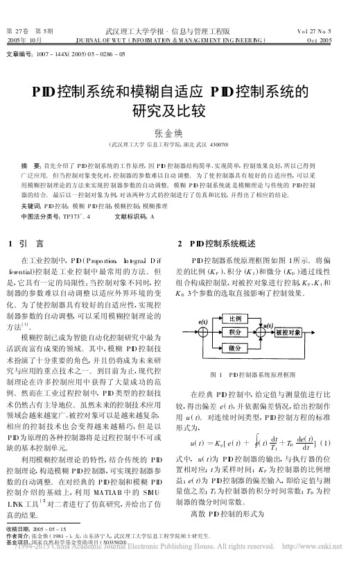
第27卷　第5期 武汉理工大学学报 信息与管理工程版 V o.l 27N o .52005年10月 J OU RNAL OF WU T (I NFO R M AT ION ＆M ANAG E M ENT E NG I NEER I NG ) O c.t 2005文章编号:1007-144X (2005)05-0286-05收稿日期:2005-05-15.作者简介:张金焕(1981-),女,山东济宁人,武汉理工大学信息工程学院硕士研究生.基金项目:国家自然科学基金资助项目(50335020).PI D 控制系统和模糊自适应PI D 控制系统的研究及比较张金焕(武汉理工大学信息工程学院,湖北武汉430070)摘　要:首先介绍了P ID 控制系统的工作原理,因P I D 控制器结构简单、实现简单,控制效果良好,所以已得到广泛应用。

但当控制对象变化时,控制器的参数难以自动调整。

为了使控制器具有较好的自适应性,可以采用模糊控制理论的方法来实现控制器参数的自动调整。

模糊P I D 控制系统就是模糊理论与传统的P ID 控制器的结合。

最后以一控制对象为例,对该两种方式的控制进行了仿真和比较,并得出了相应的结论。

关键词:P ID 控制;模糊P ID 控制;模糊控制;模糊推理中图法分类号:TP373+.4 文献标识码:A1　引　言在工业控制中,PI D (Propo rtion ,I n t e gra l ,D if -fer ential )控制是工业控制中最常用的方法。

但是,它具有一定的局限性:当控制对象不同时,控制器的参数难以自动调整以适应外界环境的变化。

为了使控制器具有较好的自适应性,实现控制器参数的自动调整,可以采用模糊控制理论的方法[1]。

模糊控制已成为智能自动化控制研究中最为活跃而富有成果的领域。

其中,模糊PI D 控制技术扮演了十分重要的角色,并且仍将成为未来研究与应用的重点技术之一。

到目前为止,现代控制理论在许多控制应用中获得了大量成功的范例。

基于LabVIEW模糊自适应PID的实现作者：齐小坤彭宇宁陆超何心孟凡钰来源：《计算技术与自动化》2011年第04期文章编号：1003-6199(2011)04-0038-摘要：通过LabVIEW与MATLAB进行混合编程的方式，借助两软件各自的优势，设计出具有模糊自适应PID控制算法的虚拟仪器，并对不同的对象特性进行控制系统的仿真与三容水箱液位的实时测控。

实验结果表明，模糊自适应PID控制系统的控制效果良好，具有较强的鲁棒性。

关键词：LabVIEW与MATLAB的混合编程；模糊自适应PID；鲁棒性；虚拟仪器中图分类号： TP273.4 文献标识码：AFuzzy Adaptive PID Realization Based on LabVIEW(School of Electrical Engineering, Guangxi University, Nanning 530004, China)Abstract:With advantage of LabVIEW and MATLAB, the paper which gets LabVIEW and MATLAB mixed, designs a fuzzy adaptive PID control algorithm of virtual instrument. It not only simulates of control system for different object characteristics, but also measures and controls three let water level of the real-time. According to the results of experiment, the effect of fuzzy adaptive PID control system control having the strong robustness is superior.PID;robustness;virtual instrument1 引言自PID算法诞生以来，以其结构简单、稳定性好、工作可靠、调整方便而成为工业应用中的首选控制策略之一，其在模型确定、线性系统中具有良好的控制效果，但在非线性、强耦合、大滞后、模型不确定的情况下则显得力不从心。

PID controller免费的百科全书Jump to: navigation, search跳转到:导航搜索A block diagram of a PID controller一个PID控制器的框图A proportional比例–integral积分–derivative 微分controller (PID controller) is a generic control loop feedback mechanism (controller) widely used in industrial control systems– a PID is the most commonly used feedback controller. A PID controller calculates an "error" value as the difference between a measured process variable and a desired setpoint. The controller attempts to minimize the error by adjusting the process control inputs.The PID controller calculation (algorithm) involves three separate constant parameters, and is accordingly sometimes called three-term control: the proportional, the integral and derivative values, denoted P,I, and D.Heuristically, these values can be interpreted in terms of time: P depends on the present error, I on the accumulation of past errors, and D is a prediction of future errors, based on current rate of change.[1] The weighted sum of these three actions is used to adjust the process via a control element such as the position of a control valve, or the power supplied to a heating element.In the absence of knowledge of the underlying process, a PID controller has historically been considered to be the best controller.[2] By tuning the three parameters in the PID controller algorithm, the controller can provide control action designed for specific process requirements. The response of the controller can be described in terms of the responsiveness of the controller to an error, the degree to which the controller overshoots the setpoint and the degree of system oscillation. Note that the use of the PID algorithm for control does not guarantee optimal control of the system or system stability.Some applications may require using only one or two actions to provide the appropriate system control. This is achieved by setting the other parameters to zero. A PID controller will be called a PI, PD, P or Icontroller in the absence of the respective control actions. PI controllers are fairly common, since derivative action is sensitive to measurement noise, whereas the absence of an integral term may prevent the system from reaching its target value due to the control action.Contents[hide]∙ 1 Control loop basics∙ 2 PID controller theoryo 2.1 Proportional term2.1.1 Droopo 2.2 Integral termo 2.3 Derivative term∙ 3 Loop tuningo 3.1 Stabilityo 3.2 Optimum behavioro 3.3 Overview of methodso 3.4 Manual tuningo 3.5 Ziegler–Nichols methodo 3.6 PID tuning software∙ 4 Modifications to the PID algorithm∙ 5 History∙ 6 Limitations of PID controlo 6.1 Linearityo 6.2 Noise in derivative∙7 Improvementso7.1 Feed-forwardo7.2 Other improvements∙8 Cascade control∙9 Physical implementation of PID control∙10 Alternative nomenclature and PID formso10.1 Ideal versus standard PID formo10.2 Basing derivative action on PVo10.3 Basing proportional action on PVo10.4 Laplace form of the PID controllero10.5 PID Pole Zero Cancellationo10.6 Series/interacting formo10.7 Discrete implementationo10.8 Pseudocode∙11 PI controller∙12 See also∙13 References∙14 External linkso14.1 PID tutorialso14.2 Special topics and PID control applications [edit] Control loop basics基本控制回路Further information更多信息: Control system控制系统A familiar example of a control loop is the action taken when adjusting hot and cold faucets (valves) to maintain the water at a desired temperature. This typically involves the mixing of two process streams, the hot and cold water. The person touches the water to sense or measure its temperature. Based on this feedback they perform a control action to adjust the hot and cold water valves until the process temperature stabilizes at the desired value.The sensed water temperature is the process variable or process value (PV). The desired temperature is called the setpoint (SP). The input to the process (the water valve position) is called the manipulated variable (MV). The difference between the temperature measurement and the set point is the error (e) and quantifies whether the water is too hot or too cold and by how much.After measuring the temperature (PV), and then calculating the error, the controller decides when to change the tap position (MV) and by how much. When the controller first turns the valve on, it may turn the hot valve only slightly if warm water is desired, or it may open the valve all the way if very hot water is desired. This is an example of a simple proportional control. In the event that hot water does not arrive quickly, the controller may try to speed-up the process by opening up the hot water valve more-and-more as time goes by. This is an example of an integral control.Making a change that is too large when the error is small is equivalent to a high gain controller and will lead to overshoot. If the controller were to repeatedly make changes that were too large and repeatedly overshoot the target, the output would oscillate around the setpoint in either a constant, growing, or decaying sinusoid. If the oscillations increase with time then the system is unstable, whereas if they decrease the system is stable. If the oscillations remain at a constant magnitude the system is marginally stable.In the interest of achieving a gradual convergence at the desired temperature (SP), the controller may wish to damp the anticipated future oscillations. So in order to compensate for this effect, the controller may elect to temper its adjustments. This can be thought of as a derivative control method.If a controller starts from a stable state at zero error (PV = SP), then further changes by the controller will be in response to changes in other measured or unmeasured inputs to the process that impact on the process, and hence on the PV. Variables that impact on the process other than the MV are known as disturbances. Generally controllers are used to reject disturbances and/or implement setpoint changes. Changes in feedwater temperature constitute a disturbance to the faucet temperature control process.In theory, a controller can be used to control any process which has a measurable output (PV), a known ideal value for that output (SP) and an input to the process (MV) that will affect the relevant PV. Controllers are used in industry to regulate temperature, pressure, flow rate, chemical composition, speed and practically every other variable for which a measurement exists.[edit] PID controller theoryThis section describes the parallel or non-interacting form of the PID controller. For other forms please see the section Alternative nomenclature and PID forms.The PID control scheme is named after its three correcting terms, whose sum constitutes the manipulated variable (MV). The proportional, integral, and derivative terms are summed to calculate the output of the PIDcontroller. Defining as the controller output, the final form of the PID algorithm is:where: Proportional gain, a tuning parameter: Integral gain, a tuning parameter: Derivative gain, a tuning parameter: Error: Time or instantaneous time (the present) [edit] Proportional termPlot of PV vs time, for three values of Kp (Kiand Kdheld constant)The proportional term makes a change to the output that is proportional to the current error value. The proportional response can be adjusted by multiplying the error by a constant K p, called the proportional gain.The proportional term is given by:A high proportional gain results in a large change in the output for a given change in the error. If the proportional gain is too high, the system can become unstable (see the section on loop tuning). In contrast, a small gain results in a small output response to a large input error, and a less responsive or less sensitive controller. If the proportional gain is too low, the control action may be too small when responding to system disturbances. Tuning theory and industrial practice indicate that the proportional term should contribute the bulk of the output change.[citation needed][edit] DroopA pure proportional controller will not always settle at its target value, but may retain a steady-state error. Specifically, drift in the absence of control, such as cooling of a furnace towards room temperature, biases a pure proportional controller. If the drift is downwards, as in cooling, then the bias will be below the set point, hence the term "droop".Droop is proportional to the process gain and inversely proportional to proportional gain. Specifically the steady-state error is given by:Droop is an inherent defect of purely proportional control. Droop may be mitigated by adding a compensating bias term (setting the setpoint above the true desired value), or corrected by adding an integral term.[edit] Integral termPlot of PV vs time, for three values of Ki (Kpand Kdheld constant)The contribution from the integral term is proportional to both the magnitude of the error and the duration of the error. The integral in a PID controller is the sum of the instantaneous error over time and gives the accumulated offset that should have been corrected previously. Theaccumulated error is then multiplied by the integral gain () and added to the controller output.The integral term is given by:The integral term accelerates the movement of the process towards setpoint and eliminates the residual steady-state error that occurs with a pure proportional controller. However, since the integral term responds to accumulated errors from the past, it can cause the present value to overshoot the setpoint value (see the section on loop tuning).[edit] Derivative termPlot of PV vs time, for three values of Kd (Kpand Kiheld constant)The derivative of the process error is calculated by determining the slope of the error over time and multiplying this rate of change by thederivative gain . The magnitude of the contribution of the derivative term to the overall control action is termed the derivative gain, . The derivative term is given by:The derivative term slows the rate of change of the controller output. Derivative control is used to reduce the magnitude of the overshoot produced by the integral component and improve the combinedcontroller-process stability. However, the derivative term slows thetransient response of the controller. Also, differentiation of a signal amplifies noise and thus this term in the controller is highly sensitive to noise in the error term, and can cause a process to become unstable if the noise and the derivative gain are sufficiently large. Hence an approximation to a differentiator with a limited bandwidth is more commonly used. Such a circuit is known as a phase-lead compensator.[edit] Loop tuningTuning a control loop is the adjustment of its control parameters (proportional band/gain, integral gain/reset, derivative gain/rate) to the optimum values for the desired control response. Stability (bounded oscillation) is a basic requirement, but beyond that, different systems have different behavior, different applications have different requirements, and requirements may conflict with one another.PID tuning is a difficult problem, even though there are only three parameters and in principle is simple to describe, because it must satisfy complex criteria within the limitations of PID control. There are accordingly various methods for loop tuning, and more sophisticated techniques are the subject of patents; this section describes some traditional manual methods for loop tuning.Designing and tuning a PID controller appears to be conceptually intuitive, but can be hard in practice, if multiple (and often conflicting) objectives such as short transient and high stability are to be achieved. Usually, initial designs need to be adjusted repeatedly through computer simulations until the closed-loop system performs or compromises as desired.Some processes have a degree of non-linearity and so parameters that work well at full-load conditions don't work when the process is starting up from no-load; this can be corrected by gain scheduling (using different parameters in different operating regions). PID controllers often provide acceptable control using default tunings, but performance can generally be improved by careful tuning, and performance may be unacceptable with poor tuning.[edit] StabilityIf the PID controller parameters (the gains of the proportional, integral and derivative terms) are chosen incorrectly, the controlled process input can be unstable, i.e., its output diverges, with or withoutoscillation, and is limited only by saturation or mechanical breakage. Instability is caused by excess gain, particularly in the presence of significant lag.Generally, stabilization of response is required and the process must not oscillate for any combination of process conditions and setpoints, though sometimes marginal stability (bounded oscillation) is acceptable or desired.[citation needed][edit] Optimum behaviorThe optimum behavior on a process change or setpoint change varies depending on the application.Two basic requirements are regulation (disturbance rejection – staying at a given setpoint) and command tracking(implementing setpoint changes) –these refer to how well the controlled variable tracks the desired value. Specific criteria for command tracking include rise time and settling time. Some processes must not allow an overshoot of the process variable beyond the setpoint if, for example, this would be unsafe. Other processes must minimize the energy expended in reaching a new setpoint.[edit] Overview of methodsThere are several methods for tuning a PID loop. The most effective methods generally involve the development of some form of process model, then choosing P, I, and D based on the dynamic model parameters. Manual tuning methods can be relatively inefficient, particularly if the loops have response times on the order of minutes or longer.The choice of method will depend largely on whether or not the loop can be taken "offline" for tuning, and the response time of the system. If the system can be taken offline, the best tuning method often involves subjecting the system to a step change in input, measuring the output as a function of time, and using this response to determine the control parameters.Choosing a Tuning MethodMethod Advantages DisadvantagesManual Tuning No math required. Online method. Requires experienced personnel.Ziegler–Nichols Proven Method. Online method. Process upset, sometrial-and-error, veryaggressive tuning.Software Tools Consistent tuning. Online oroffline method. May includevalve and sensor analysis. Allow simulation before downloading. Can support Non-Steady State(NSS) Tuning.Some cost and training involved.Cohen-Coon Good process models. Some math. Offline method. Only good forfirst-order processes.[edit ] Manual tuningIf the system must remain online, one tuning method is to first set and values to zero. Increase the until the output of the loop oscillates, then the should be set to approximately half of that valuefor a "quarter amplitude decay" type response. Then increaseuntil any offset is corrected in sufficient time for the process. However, too muchwill cause instability. Finally, increase , if required, until the loop is acceptably quick to reach its reference after a load disturbance. However, too much will cause excessive response and overshoot. A fast PID loop tuning usually overshoots slightly to reach the setpoint more quickly; however, some systems cannot accept overshoot, in which case an over-damped closed-loop system is required, which will require a setting significantly less than half that of the setting causing oscillation. Effects of increasing a parameter independently Parameter Rise time OvershootSettlingtime Steady-state error Stability [3] Decrease Increase Smallchange DecreaseDegrade Decrease [4] Increase Increase Decrease DegradesignificantlyMinor decrease Minor decrease Minor decrease No effect intheory Improve if small[edit ] Ziegler –Nichols methodFor more details on this topic, see Ziegler –Nichols method .Another heuristic tuning method is formally known asthe Ziegler –Nichols method , introducedbyJohnG.ZieglerandNathaniel B. Nichols in the 1940s. As in the method above, the and gains are first set to zero. TheP gain is increased until it reaches the ultimate gain,, at which the output of the loop starts to oscillate.and the oscillation periodare used to set the gains as shown:Ziegler –Nichols methodControl Type P- - PI-PID These gains apply to the ideal, parallel form of the PID controller. When applied to the standard PID form, the integral and derivative time parameters and are only dependent on the oscillation period . Please see the section "Alternative nomenclature and PID forms ".[edit ] PID tuning softwareMost modern industrial facilities no longer tune loops using the manual calculation methods shown above. Instead, PID tuning and loopoptimization software are used to ensure consistent results. These software packages will gather the data, develop process models, andsuggest optimal tuning. Some software packages can even develop tuning by gathering data from reference changes.Mathematical PID loop tuning induces an impulse in the system, and then uses the controlled system's frequency response to design the PID loop values. In loops with response times of several minutes, mathematical loop tuning is recommended, because trial and error can take days just to find a stable set of loop values. Optimal values are harder to find. Some digital loop controllers offer a self-tuning feature in which very small setpoint changes are sent to the process, allowing the controller itself to calculate optimal tuning values.Other formulas are available to tune the loop according to different performance criteria. Many patented formulas are now embedded within PID tuning software and hardware modules.Advances in automated PID Loop Tuning software also deliver algorithms for tuning PID Loops in a dynamic or Non-Steady State (NSS) scenario. The software will model the dynamics of a process, through a disturbance, and calculate PID control parameters in response.[edit] Modifications to the PID algorithmThe basic PID algorithm presents some challenges in control applications that have been addressed by minor modifications to the PID form.Integral windupFor more details on this topic, see Integral windup.One common problem resulting from the ideal PID implementations is integral windup, where a large change in setpoint occurs (say a positive change) and the integral term accumulates an error larger than the maximal value for the regulation variable (windup), thus the system overshoots and continues to increase as this accumulated error is unwound. This problem can be addressed by:∙Initializing the controller integral to a desired value∙Increasing the setpoint in a suitable ramp∙Disabling the integral function until the PV has entered the controllable region∙Limiting the time period over which the integral error is calculated ∙Preventing the integral term from accumulating above or below pre-determined boundsOvershooting from known disturbancesFor example, a PID loop is used to control the temperature of an electric resistance furnace, the system has stabilized. Now the door is opened and something cold is put into the furnace thetemperature drops below the setpoint. The integral function of the controller tends to compensate this error by introducing another error in the positive direction. This overshoot can be avoided by freezing of the integral function after the opening of the door for the time the control loop typically needs to reheat the furnace. Replacing the integral function by a model based partOften the time-response of the system is approximately known. Then it is an advantage to simulate this time-response with a model and to calculate some unknown parameter from the actual response of the system. If for instance the system is an electrical furnace the response of the difference between furnace temperature and ambient temperature to changes of the electrical power will be similar to that of a simple RC low-pass filter multiplied by an unknownproportional coefficient. The actual electrical power supplied to the furnace is delayed by a low-pass filter to simulate the response of the temperature of the furnace and then the actual temperature minus the ambient temperature is divided by this low-pass filtered electrical power. Then, the result is stabilized by anotherlow-pass filter leading to an estimation of the proportionalcoefficient. With this estimation, it is possible to calculate the required electrical power by dividing the set-point of thetemperature minus the ambient temperature by this coefficient. The result can then be used instead of the integral function. This also achieves a control error of zero in the steady-state, but avoids integral windup and can give a significantly improved controlaction compared to an optimized PID controller. This type ofcontroller does work properly in an open loop situation which causes integral windup with an integral function. This is an advantage if, for example, the heating of a furnace has to be reduced for some time because of the failure of a heating element, or if thecontroller is used as an advisory system to a human operator who may not switch it to closed-loop operation. It may also be useful if the controller is inside a branch of a complex control system that may be temporarily inactive.Many PID loops control a mechanical device (for example, a valve). Mechanical maintenance can be a major cost and wear leads to control degradation in the form of either stiction or a deadband in the mechanical response to an input signal. The rate of mechanical wear is mainly a function of how often a device is activated to make a change. Where wearis a significant concern, the PID loop may have an output deadband to reduce the frequency of activation of the output (valve). This is accomplished by modifying the controller to hold its output steady if the change would be small (within the defined deadband range). The calculated output must leave the deadband before the actual output will change.The proportional and derivative terms can produce excessive movement in the output when a system is subjected to an instantaneous step increase in the error, such as a large setpoint change. In the case of the derivative term, this is due to taking the derivative of the error, which is very large in the case of an instantaneous step change. As a result, some PID algorithms incorporate the following modifications:Derivative of the Process VariableIn this case the PID controller measures the derivative of themeasured process variable (PV), rather than the derivative of the error. This quantity is always continuous (i.e., never has a step change as a result of changed setpoint). For this technique to be effective, the derivative of the PV must have the opposite sign of the derivative of the error, in the case of negative feedbackcontrol.Setpoint rampingIn this modification, the setpoint is gradually moved from its old value to a newly specified value using a linear or first orderdifferential ramp function. This avoids the discontinuity present in a simple step change.Setpoint weightingSetpoint weighting uses different multipliers for the errordepending on which element of the controller it is used in. The error in the integral term must be the true control error to avoidsteady-state control errors. This affects the controller'ssetpoint response. These parameters do not affect the response to load disturbances and measurement noise.[edit] HistoryThis section requires expansion.PID theory developed by observing the action of helmsmen.PID controllers date to 1890s governor design.[2][5] PID controllers were subsequently developed in automatic ship steering. One of the earliest examples of a PID-type controller was developed by Elmer Sperry in 1911,[6] while the first published theoretical analysis of a PID controller was by Russian American engineer Nicolas Minorsky, in (Minorsky 1922). Minorsky was designing automatic steering systems for the US Navy, and based his analysis on observations of a helmsman, observing that the helmsman controlled the ship not only based on the current error, but also on past error and current rate of change;[7]this was then made mathematical by Minorsky. His goal was stability, not general control, which significantly simplified the problem. While proportional control provides stability against small disturbances, it was insufficient for dealing with a steady disturbance, notably a stiff gale (due to droop), which required adding the integral term. Finally, the derivative term was added to improve control.Trials were carried out on the USS New Mexico, with the controller controlling the angular velocity (not angle) of the rudder. PI control yielded sustained yaw (angular error) of ±2°, while adding D yielded yaw of ±1/6°, better than most helmsmen could achieve.[8]The Navy ultimately did not adopt the system, due to resistance by personnel. Similar work was carried out and published by several others in the 1930s.[edit] Limitations of PID controlWhile PID controllers are applicable to many control problems, and often perform satisfactorily without any improvements or even tuning, they can perform poorly in some applications, and do not in general provide optimal control. The fundamental difficulty with PID control is that it is a feed back system, with constant parameters, and no direct knowledge of the process, and thus overall performance is reactive and a compromise –while PID control is the best controller with no model of the process,[2] better performance can be obtained by incorporating a model of the process.The most significant improvement is to incorporate feed-forward control with knowledge about the system, and using the PID only to control error. Alternatively, PIDs can be modified in more minor ways, such as by changing the parameters (either gain scheduling in different use cases or adaptively modifying them based on performance), improving measurement (higher sampling rate, precision, and accuracy, and low-pass filtering if necessary), or cascading multiple PID controllers.PID controllers, when used alone, can give poor performance when the PID loop gains must be reduced so that the control system does not overshoot, oscillate or hunt about the control setpoint value. They also have difficulties in the presence of non-linearities, may trade-off regulation versus response time, do not react to changing process behavior (say, the process changes after it has warmed up), and have lag in responding to large disturbances.[edit] LinearityAnother problem faced with PID controllers is that they are linear, and in particular symmetric. Thus, performance of PID controllers innon-linear systems (such as HVAC systems) is variable. For example, in temperature control, a common use case is active heating (via a heating element) but passive cooling (heating off, but no cooling), so overshoot can only be corrected slowly –it cannot be forced downward. In this case the PID should be tuned to be overdamped, to prevent or reduce overshoot, though this reduces performance (it increases settling time).[edit] Noise in derivativeA problem with the derivative term is that small amounts of measurement or process noise can cause large amounts of change in the output. It is often helpful to filter the measurements with a low-pass filter in order to remove higher-frequency noise components. However, low-pass filtering and derivative control can cancel each other out, so reducing noise by instrumentation is a much better choice. Alternatively, a nonlinear median filter may be used, which improves the filtering efficiency and practical performance.[9]In some case, the differential band can be turned off in many systems with little loss of control. This is equivalent to using the PID controller as a PI controller.。

附件1：外文原文PID controllerZuo Xin and Sun Jinming(Research Institute ofAutomation, University of Petroleum,Belting 102249,China)Received April 2，2005Abstract:Performance assessment of a proportional-integral-derivative(PID)controller is condueted using the PID achievable minimum variance as abenchmark．When the process model is unknown，we carl estimate the P／D·achievable minimum variance and the corresponding parameters by routine closed-loop operation data．Simulation results show that the process output variance is reduced by retuning controller parameters．Key words：Performance assessment，PID control，minimum varianceA proportional–integral–derivative controller (PID controller) is a generic .control loop feedback mechanism widely used in industrial control systems.A PID controller attempts to correct the error between a measured process variable and a desired setpoint by calculating and then outputting a corrective action that can adjust the process accordingly.The PID controller calculation (algorithm) involves three separate parameters; the Proportional, the Integral and Derivative values. The Proportional value determines the reaction to the current error, the Integral determines the reaction based on the sum of recent errors and the Derivative determines the reaction to the rate at which the error has been changing. The weightedsum of these three actions is used to adjust the process via a control element such as the position of a control valve or the power supply of a heating element.By "tuning" the three constants in the PID controller algorithm the PID can provide control action designed for specific process requirements. The response of the controller can be described in terms of the responsiveness of the controller to an error, the degree to which the controller overshoots the setpoint and the degree of system oscillation. Note that the use of the PID algorithm for control does not guarantee optimal control of the system or systemstability.Some applications may require using only one or two modes to provide the appropriate system control. This is achieved by setting the gain of undesired control outputs to zero. A PID controller will be called a PI, PD, P or I controller in the absence of the respective control actions. PI controllers are particularly common, since derivative action is very sensitive to measurement noise, and the absence of an integral value may prevent the system from reaching its target value due to the control action.Note: Due to the diversity of the field of control theory and application, many naming conventions for the relevant variables are in common use.1.Control loop basicsA familiar example of a control loop is the action taken to keep one's shower water at the ideal temperature, which typically involves the mixing of two process streams, cold and hot water. The person feels the water to estimate its temperature. Based on this measurement they perform a control action: use the cold water tap to adjust the process. The person would repeat this input-output control loop, adjusting the hot water flow until the process temperature stabilized at the desired value.Feeling the water temperature is taking a measurement of the process value or process variable (PV). The desired temperature is called the setpoint (SP). The output from the controller and input to the process (the tap position) is called the manipulated variable (MV). The difference between the measurement and the setpoint is the error (e), too hot or too cold and by how much.As a controller, one decides roughly how much to change the tap position (MV) after one determines the temperature (PV), and therefore the error. This first estimate is the equivalent of the proportional action of a PID controller. The integral action of a PID controller can be thought of as gradually adjusting the temperature when it is almost right. Derivative action can be thought of as noticing the water temperature is getting hotter or colder, and how fast, and taking that into account when deciding how to adjust the tap.Making a change that is too large when the error is small is equivalent to a high gain controller and will lead toovershoot. If the controller were to repeatedly make changes that were too large and repeatedly overshoot the target, this control loop would be termed unstable and the output would oscillate around the setpoint in either a constant, growing, or decaying sinusoid. A human would not do this because we are adaptive controllers, learning from the process history, but PID controllers do not have the ability to learn and must be set up correctly. Selecting the correct gains for effective control is known as tuning the controller.If a controller starts from a stable state at zero error (PV = SP), then further changes by the controller will be in response to changes in other measured or unmeasured inputs to the process that impact on the process, and hence on the PV. Variables that impact on the process other than the MV are known as disturbances and generally controllers are used to reject disturbances and/or implement setpoint changes. Changes in feed water temperature constitute a disturbance to the shower process.In theory, a controller can be used to control any process which has a measurable output (PV), a known ideal value for that output (SP) and an input to the process (MV) that will affect the relevant PV. Controllers are used in industry to regulate temperature, pressure, flow rate, chemical composition, speed and practically every other variable for which a measurement exists. Automobile cruise control is an example of a process which utilizes automated control.Due to their long history, simplicity, well grounded theory and simple setup and maintenance requirements, PID controllers are the controllers of choice for many of these applications.2.PID controller theoryNote: This section describes the ideal parallel or non-interacting form of the PID controller. For other forms please see the Section "Alternative notation and PID forms".The PID control scheme is named after its three correcting terms, whose sum constitutes the manipulated variable (MV). Hence:Where Pout, Iout, and Dout are the contributions to the output from the PID controller from each of the three terms, as defined below.2.1. Proportional termThe proportional term makes a change to the output that is proportional to the current error value. The proportional response can be adjusted by multiplying the error by a constant Kp, called the proportional gain.The proportional term is given by:WherePout: Proportional outputKp: Proportional Gain, a tuning parametere: Error = SP − PVt: Time or instantaneous time (the present)Change of response for varying KpA high proportional gain results in a large change in the output for a given change in the error. If the proportional gain is too high, the system can become unstable (See the section on Loop Tuning). In contrast, a small gain results in a small output response to a large input error, and a less responsive (or sensitive) controller. If the proportional gain is too low, the control action may be too small when responding to system disturbances.In the absence of disturbances, pure proportional control will not settle at its target value, but will retain a steady state error that is a function of the proportional gain and the process gain. Despite the steady-state offset, both tuning theory and industrial practice indicate that it is the proportional term that should contribute the bulk of the output change.2.2.Integral termThe contribution from the integral term is proportional to both the magnitude of the error and the duration of the error. Summing the instantaneous error over time (integrating the error) gives the accumulated offset that should have been correctedpreviously. The accumulated error is then multiplied by the integral gain and added to the controller output. The magnitude of the contribution of the integral term to the overall control action is determined by the integral gain, Ki.The integral term is given by:Iout: Integral outputKi: Integral Gain, a tuning parametere: Error = SP − PVτ: Time in the past contributing to the integral responseThe integral term (when added to the proportional term) accelerates the movement of the process towards setpoint and eliminates the residual steady-state error that occurs with a proportional only controller. However, since the integral term is responding to accumulated errors from the past, it can cause the present value to overshoot the setpoint value (cross over the setpoint and then create a deviation in the other direction). For further notes regarding integral gain tuning and controller stability, see the section on loop tuning.2.3 Derivative termThe rate of change of the process error is calculated by determining the slope of the error over time (i.e. its first derivative with respect to time) and multiplying this rate of change by the derivative gain Kd. The magnitude of the contribution of the derivative term to the overall control action is termed the derivative gain, Kd.The derivative term is given by:Dout: Derivative outputKd: Derivative Gain, a tuning parametere: Error = SP − PVt: Time or instantaneous time (the present)The derivative term slows the rate of change of the controller output and this effect is most noticeable close to the controller setpoint. Hence, derivative control is used to reduce the magnitude of the overshoot produced by the integral component and improve the combined controller-process stability. However, differentiation of a signal amplifies noise and thus this term in the controller is highly sensitive to noise in the error term, and can cause a process to become unstable if the noise and the derivative gain are sufficiently large.2.4 SummaryThe output from the three terms, the proportional, the integral and the derivative terms are summed to calculate the output of the PID controller. Defining u(t) as the controller output, the final form of the PID algorithm is:and the tuning parameters areKp: Proportional Gain - Larger Kp typically means faster response since thelarger the error, the larger the Proportional term compensation. An excessively large proportional gain will lead to process instability and oscillation.Ki: Integral Gain - Larger Ki implies steady state errors are eliminated quicker. The trade-off is larger overshoot: any negative error integrated during transient response must be integrated away by positive error before we reach steady state.Kd: Derivative Gain - Larger Kd decreases overshoot, but slows down transient response and may lead to instability due to signal noise amplification in the differentiation of the error.3. Loop tuningIf the PID controller parameters (the gains of the proportional, integral and derivative terms) are chosen incorrectly, the controlled process input can be unstable, i.e. its output diverges, with or without oscillation, and is limited only by saturation or mechanical breakage. Tuning a control loop is the adjustment of its control parameters (gain/proportional band, integral gain/reset, derivative gain/rate) to the optimumvalues for the desired control response.The optimum behavior on a process change or setpoint change varies depending on the application. Some processes must not allow an overshoot of the process variable beyond the setpoint if, for example, this would be unsafe. Other processes must minimize the energy expended in reaching a new setpoint. Generally, stability of response (the reverse of instability) is required and the process must not oscillate for any combination of process conditions and setpoints. Some processes have a degree of non-linearity and so parameters that work well at full-load conditions don't work when the process is starting up from no-load. This section describes some traditional manual methods for loop tuning.There are several methods for tuning a PID loop. The most effective methods generally involve the development of some form of process model, then choosing P, I, and D based on the dynamic model parameters. Manual tuning methods can be relatively inefficient.The choice of method will depend largely on whether or not the loop can be taken "offline" for tuning, and the response time of the system. If the system can be taken offline, the best tuning method often involves subjecting the system to a step change in input, measuring the output as a function of time, and using this response to determine the control parameters.Choosing a Tuning MethodMethodAdvantagesDisadvantagesManual TuningNo math required. Online method.Requires experiencedpersonnel.Ziegler–NicholsProven Method. Online method.Process upset, sometrial-and-error, very aggressive tuning.Software ToolsConsistent tuning. Online or offline method. May includevalve and sensor analysis. Allow simulation before downloading.Some cost and training involved.Cohen-CoonGood process models.Some math. Offline method. Onlygood for first-order processes.3.1 Manual tuningIf the system must remain online, one tuning method is to first set the I and D values to zero. Increase the P until the output of the loop oscillates, then the P should be left set to be approximately half of that value for a "quarter amplitude decay" type response. Then increase D until any offset is correct in sufficient time for the process. However, too much D will cause instability. Finally, increase I, if required, until the loop is acceptably quick to reach its reference after a load disturbance. However, too much I will cause excessive response and overshoot. A fast PID loop tuning usually overshoots slightly to reach the setpoint more quickly; however, some systems cannot accept overshoot, in which case an "over-damped" closed-loop system is required, which will require a P setting significantly less than half that of the P setting causing oscillation.3.2Ziegler–Nichols methodAnother tuning method is formally known as the Ziegler–Nichols method, introduced by John G. Ziegler and Nathaniel B. Nichols. As in the method above, the I and D gains are first set to zero. The "P" gain is increased until it reaches the "critical gain" Kc at which the output of the loop starts to oscillate. Kc and the oscillation period Pc are used to set the gains as shown:3.3 PID tuning softwareMost modern industrial facilities no longer tune loops using the manual calculation methods shown above. Instead, PID tuning and loop optimization software are used to ensure consistent results. These software packages will gather the data, develop process models, and suggest optimal tuning. Some software packages can even develop tuning by gathering data from reference changes.Mathematical PID loop tuning induces an impulse in the system, and then uses the controlled system's frequency response to design the PID loop values. In loops with response times of several minutes, mathematical loop tuning is recommended, because trial and error can literally take days just to find a stable set of loop values.Optimal values are harder to find. Some digital loop controllers offer a self-tuning feature in which very small setpoint changes are sent to the process, allowing the controller itself to calculate optimal tuning values.Other formulas are available to tune the loop according to different performance criteria.4 Modifications to the PID algorithmThe basic PID algorithm presents some challenges in control applications that have been addressed by minor modifications to the PID form.One common problem resulting from the ideal PID implementations is integralwindup. This can be addressed by:Initializing the controller integral to a desired valueDisabling the integral function until the PV has entered the controllable region Limiting the time period over which the integral error is calculatedPreventing the integral term from accumulating above or below pre-determined boundsMany PID loops control a mechanical device (for example, a valve). Mechanical maintenance can be a major cost and wear leads to control degradation in the form of either stiction or a deadband in the mechanical response to an input signal. The rate of mechanical wear is mainly a function of how often a device is activated to make a change. Where wear is a significant concern, the PID loop may have an output deadband to reduce the frequency of activation of the output (valve). This is accomplished by modifying the controller to hold its output steady if the change would be small (within the defined deadband range). The calculated output must leave the deadband before the actual output will change.The proportional and derivative terms can produce excessive movement in the output when a system is subjected to an instantaneous "step" increase in the error, such as a large setpoint change. In the case of the derivative term, this is due to taking the derivative of the error, which is very large in the case of an instantaneous step change.5. Limitations of PID controlWhile PID controllers are applicable to many control problems, they can perform poorly in some applications.PID controllers, when used alone, can give poor performance when the PID loop gains must be reduced so that the control system does not overshoot, oscillate or "hunt" about the control setpoint value. The control system performance can be improved by combining the feedback (or closed-loop) control of a PID controller with feed-forward (or open-loop) control. Knowledge about the system (such as the desired acceleration and inertia) can be "fed forward" and combined with the PID output to improve the overall system performance. The feed-forward value alone can often provide the major portion of the controller output. The PID controller can then be used primarily to respond to whatever difference or "error" remains between the setpoint (SP) and the actual value of the process variable (PV). Since the feed-forward output is not affected by the process feedback, it can never cause the control system to oscillate, thus improving the system response and stability.For example, in most motion control systems, in order to accelerate a mechanical load under control, more force or torque is required from the prime mover, motor, or actuator. If a velocity loop PID controller is being used to control the speed of the load and command the force or torque being applied by the prime mover, then it is beneficial to take the instantaneous acceleration desired for the load, scale that value appropriately and add it to the output of the PID velocity loop controller. This means that whenever the load is being accelerated or decelerated, a proportional amount of force is commanded from the prime mover regardless of the feedback value. The PID loop in this situation uses the feedback information to effect any increase or decrease of the combined output in order to reduce the remaining difference between the process setpoint and thefeedback value. Working together, the combined open-loop feed-forward controller and closed-loop PID controller can provide a more responsive, stable and reliable control system.Another problem faced with PID controllers is that they are linear. Thus, performance of PID controllers in non-linear systems (such as HV AC systems) isvariable. Often PID controllers are enhanced through methods such as PID gain scheduling or fuzzy logic. Further practical application issues can arise from instrumentation connected to the controller. A high enough sampling rate, measurement precision, and measurement accuracy are required to achieve adequate control performance.A problem with the Derivative term is that small amounts of measurement or process noise can cause large amounts of change in the output. It is often helpful to filter the measurements with a low-pass filter in order to remove higher-frequency noise components. However, low-pass filtering and derivative control can cancel each other out, so reducing noise by instrumentation means is a much better choice. Alternatively, the differential band can be turned off in many systems with little loss of control. This is equivalent to using the PID controller as a PI controller.6. Cascade controlOne distinctive advantage of PID controllers is that two PID controllers can be used together to yield better dynamic performance. This is called cascaded PID control. In cascade control there are two PIDs arranged with one PID controlling the set point of another. A PID controller acts as outer loop controller, which controls the primary physical parameter, such as fluid level or velocity. The other controller acts as inner loop controller, which reads the output of outer loop controller as set point, usually controlling a more rapid changing parameter, flowrate or accelleration. It can be mathematically proved that the working frequency of the controller is increased and the time constant of the object is reduced by using cascaded PID controller.[vague]7. Physical implementation of PID controlIn the early history of automatic process control the PID controller was implemented as a mechanical device. These mechanical controllers used a lever, spring and a mass and were often energized by compressed air. These pneumatic controllers were once the industry standard.Electronic analog controllers can be made from a solid-state or tube amplifier, a capacitor and a resistance. Electronic analogPID control loops were often found within more complex electronic systems, for example, the head positioning of a disk drive, the power conditioning of a power supply, or even the movement-detection circuit of a modern seismometer. Nowadays, electronic controllers have largely been replaced by digital controllers implemented with microcontrollers or FPGAs.Most modern PID controllers in industry are implemented in software in programmable logic controllers (PLCs) or as a panel-mounted digital controller. Software implementations have the advantages that they are relatively cheap and are flexible with respect to the implementation of the PID algorithm.References[1]Byung，S.K.(2000)On Performance Assessment of Feedback Control Loops．Austin：The University of Texas Austin[2]Desborough，L．and Harris，T.(1992)Performance Assessment Measures for Univariate Feedback Control. The Canadian Journal of Chemical Engineering,70(12)．1186-1197[3]Ender,D.B.(1993)Process Control Performance：Not as Good as You Think．Control Engineering，40(10)[4]Harris,T(1993)Pefformance Assessment Measllres for Univariate Feedforward/Feedback Control．The Canadian Journal of Chemical Engineering，71(8)，1186-1197[5]Qin，S．J．(1 998)Contr01 Performance Monitoring： A Review and Assessment．Com．Chem．Eng．，(23)，173．186[6]Sun,Jinming(2004)PID Performance Assessment and Parameters Tuning．Beijing：China University of Petroleum[7]Xu，Xi；Li，Tao and Bo，Xiaochen(2000)Matlab Toolbox Application--Control Engineering．Bering：Electron Industry Press附件2：外文资料翻译译文PID控制器左信孙金明（石油大学自动化研究所，北京，102249，中国）发表于2005.4.2摘要：一个比例积分微分（PID）控制器的性能评价进行使用PID实现的最小方差作为参照。

步进电机模糊pid算法基本原理,c语言实现模糊PID（Proportional-Integral-Derivative）控制算法结合了模糊逻辑和传统PID控制算法，旨在提高系统的鲁棒性和稳定性。

步进电机作为一种常见的执行器，可以通过模糊PID算法实现精确的位置控制。

以下是模糊PID算法的基本原理以及C语言实现的简要步骤：模糊PID算法基本原理：1.模糊化输入和输出：将系统的输入（误差）和输出（控制量）进行模糊化，将其转换为模糊集合。

2.模糊规则库：建立模糊规则库，其中包含了一系列模糊规则，用于描述输入与输出之间的关系。

这些规则可以根据经验知识或系统模型来确定。

3.模糊推理：通过模糊规则库对模糊化的输入进行推理，得到模糊输出。

通常采用最大最小原则或加权平均等方法进行推理。

4.去模糊化：将模糊输出转换为确定性的控制量，即进行去模糊化操作。

常用的方法包括最大隶属度法、加权平均法等。

5.PID调节器：利用模糊输出和经典PID控制算法相结合，调节系统的控制量，使系统达到期望的运行状态。

C语言实现步骤：1.模糊化输入和输出：定义输入误差和输出控制量的模糊集合，并实现模糊化函数。

2.模糊规则库：定义一系列模糊规则，描述输入和输出之间的关系。

3.模糊推理：根据输入误差和模糊规则库进行推理，得到模糊输出。

4.去模糊化：实现去模糊化函数，将模糊输出转换为确定性的控制量。

5.PID调节器：结合经典PID控制算法，根据模糊输出和去模糊化后的控制量进行调节。

以下是一个简单的C语言实现示例：// 模糊化函数float fuzzyfication(float error) {// 省略具体实现，根据误差值计算归属度return fuzzy_value;}// 模糊规则库float fuzzy_rule(float error) {// 省略具体实现，定义模糊规则return fuzzy_output;}// 去模糊化函数float defuzzyfication(float fuzzy_output) {// 省略具体实现，根据模糊输出计算确定性的控制量return control_output;}int main() {float error = 0.0; // 输入误差float fuzzy_input = fuzzyfication(error); // 模糊化输入float fuzzy_output = fuzzy_rule(fuzzy_input); // 模糊推理float control_output = defuzzyfication(fuzzy_output); // 去模糊化输出// 利用确定性的控制量进行PID调节// 省略PID控制算法的实现// 控制步进电机运动return 0;}在实际应用中，模糊PID算法需要根据具体的系统和需求进行调试和优化，以实现良好的控制效果。

摘要由于变频技术的出现，交流调速一直冲击直流调速，但综观全局，尤其是我国在此领域的现状，再加上全数字直流调速系统的出现，提高了直流调速系统的精度及可靠性，直流调速仍将处于重要地位。

对于直流调速系统转速控制的要求有稳速、调速、加速或减速三个方面，而在工业生产中对于后两个要求已能很好地实现，但工程应用中稳速指标却往往不能达到预期的效果，稳速要求即以一定的精度在所需要的转速上稳定运行，在各种干扰下不允许有过大的转速波动。

稳速很难达到要求原因在于数字直流调速装置中的PID调节器对被控对象及其负载参数变化自适应能力差。

模糊控制不要求被控对象的精确模型且适应性强，为了克服常规数字直流调速装置的缺点，本文将模糊控制与PID调节器结合，着手fuzzy-PID复合控制方案理论研究和硬件的实现，设计出相关控制方案的直流调速系统，该方案以AT89C51单片机为主控单元，合适的驱动电路和一些外围电路构成硬件系统；以参数模糊自整定PID为控制策略。

本文对于系统的硬件及软件设计进行了详细的设计，包括电机控制模块、检测模块、电机驱动模块的设计等，以及软件的控制思想和编程方法。

本系统的设计顺应了目前国外直流调速朝着数字化，发展的趋势，充分利用了单片机的优点，使得通用性得到了提高。

经过理论分析和设计此控制器的各项性能指标优于模糊控制器和常规PID 控制器，具有很强的鲁棒性。

关键词：模糊控制；直流调速；稳态性能；单片机AbstractAfter Frequency Conversion Technology appeared，AC speed regulation method had always impacted DC Speed Regulation，but Generally speaking，especially the status in our country，in addition to digital DC Speed Regulation emerged，it improving the precision and the reliability in DC Speed Regulation System．DC Speed Regulation was also in the important status．Speed stability、speed ratio、acceleration、deceleration are the four factors in DC Speed Regulation System，the last two factors already reached well in industry application．But the Stability index does not match the desired purpose．Stability index is that the DC motor running in the precision range on desired speed，even if the system has uncertain disturbance．It is hard to realize because of adaptiveability digital DC Speed Regulation device is not enough when in the condition of the load parameters change unpredictably．Fuzzy control does not need precision mathematic model to conquer the shortcoming in routine digital DC Speed Regulation．We can combine with the PID adjuster and fuzzy control，focusing on theory research and realization of fuzzy-PID compound control scheme，design relevant DC Speed Regulation System was designed in the dissertation．This scheme is based on the core of AT89C51 single chip，appropriate driver circuit and some peripheral circuits，Fuzzy Self-tuning PID is the control strategy,This dissertation also introduce the plan of hardware and software，including DC motor control module、driver module、examine circuit and so on in detail，if explained the method of control and the thought of software，this system got used to the trend of digital power in the international，used the single micro—computer fully，and improveed the general use of the power．Theoretical analysis and design showed that all performance indexes of Parameter Self-Adjusting Fuzzy Logic PID Controller was in advance of those of the simple fuzzy controller and the conventional PID controller．Especially，the adaptive fuzzy controller is robust．Keywords：fuzzy logic control(FLC)；DC Speed Regulation；stability performance；Single micro-computer目 录摘 要 .................................................................................................................................................I Abstract ......................................................................................................................................... II 目 录 ............................................................................................................................................ I II第一章 绪论 (1)1.1 序言 (1)1.2 PID 控制中存在的问题 (1)1.3 模糊控制的发展状况 (2)模糊控制的发展过程 (2)模糊控制技术要解决的问题 (3)1.4 直流调速系统的发展概况 (4)1.5 本课题的研究内容及目的 (5)第二章 直流调速系统的理论分析 (6)2.1 控制理论在调速系统中的应用分析 (6)调速系统性能指标 (6)直流调速常用的方法 (7)2.2 传统直流调速系统中调节器参数的计算 (9)设计指标及要求 (9)固有、预置参数计算 (9)电流调节器参数计算 (10)转速调节器参数 (10)2.3 数字PID 调节器的原理及应用 (12)2.4 数字PID 控制器的算法实现 (14)第三章 模糊PID 控制算法设计 (16)3.1 模糊控制的原理 (16)模糊控制的理论基础 (16)模糊控制系统的组成 (16)模糊控制在实际中的适用性 (17)3.1.4 模糊控制器的设计方法 (17)3.2直流调速系统模糊PID 控制结构设计 .......................................................................... 18 被控过程对参数P K 、I K 、D K 的自整定要求 (19)3.3模糊自整定PID 参数控器设计 (20)确定控制器的输入、输出语言变量 (20)3.3.2确定各语言变量论域，在其论域上定义模糊量 .............................................. 21 确定P K 、I K 、D K 的调节规则 .. (21)模糊推理和模糊运算 (22)第四章 调速系统硬件设计 (24)4.1硬件总体方案设计 (24)4.2 主电路设计 (24)4.3 整流电力二极管参数的确定 (25)4.4 IGBT 的选择 (26)4.5 IGBT 驱动电路的设计 (26)IGBT 驱动电路的一般要求 (26)IGBT 的专用驱动集成电路 (26)4.6 泵升电压的抑制 (28)4.7 电流反馈信号检测装置设计 (29)概述 (29)4.7.2 电流检测装置的设计 (30)4.8转速检测环节及其与单片机接口电路的设计 (30)4.9 模拟量给定电流、转速反馈量与单片机的接口设计 (32)4.10 键盘与显示接口电路 (32)第五章系统软件设计 (34)5.1主程序 (34)5.2 A/D转换设计 (35)5.3键盘与显示子程序设计 (36)5.4模糊PID控制流程设计 (37)结论 (38)参考文献 (39)致谢 (42)第一章绪论1.1 序言在现代化的工业生产过程中，几乎无处不使用电力传动装置，生产工艺、产品质量的要求不断提高和产量的增长，使得越来越多的生产机械要求能实现自动调速。

1引言近年来电动执行器系统的控制策略得到了越来越多的研究，对系统的稳定运行发挥着关键作用。

电动执行器系统的控制方案主要包括驱动电机以及系统主要单元的控制策略。

系统需要提供相当多的转矩和转速，以控制阀门开度。

对于系统的动态调节，其响应速度应该相对够快，以达到系统控制精度要求。

传统阀门位置控制常采用PID 方法，该方案是基于比例、积分、微分输出控制量，来实现对系统的准确控制，具有相对简单、容易实现等特点。

然而，当被控对象的环境经常变化，即需频繁调整控制参数，对该方法的实际应用提出了限制。

因此，需要对以往的PID 策略进行改进，一种方案是改进传统控制结构，另一种则是采用智能控制方法[1]。

文献[2]研究了PID 控制方案，针对电子液压制动系统下电动执行器调节阀的控制，电动执行器流量调节阀采用传统的控制方法即可实现输出流量精确、快速的跟踪，然而系统具有较差的鲁棒性。

文献[3]采用校正控制，进一步减小了系统超调及稳态误差，大大提升了执行器系统的响应速度和抗扰动能力，并且明显改善了回差。

文献[4]研究了基于增量一种基于模糊自适应PID 的电动执行器智能控制方法李伟华（苏州博睿测控设备有限公司，苏州215143）摘要:电动执行器的系统控制方案研究在近年有较大进展。

传统控制方案基于PID 的控制策略易于在通常的实际控制系统中实现，但对于控制系统复杂程度较高的场合，传统控制方法已不能适应系统鲁棒性和实时性的要求。

为解决此问题，提出基于模糊自适应PID 的执行器系统智能控制方案。

实验结果表明，新方案有较好的动态表现以及较快的响应，并且具有较高的调节准确度，能够实现PID 参数的在线自调整，实时性更好，控制精度和鲁棒性更高，参数计算负荷小，设计方法易于实现。

关键词：模糊控制；自适应；PID 控制；智能控制DOI ：10.3969/j.issn.1002-2279.2021.02.015中图分类号:TP273+.4文献标识码:A 文章编号：1002-2279（2021）02-0058-04An Intelligent Control Method of Electric Actuator Based onFuzzy Adaptive PIDLI Weihua(Suzhou Bonray Measurement&Control Equipment Co.,Ltd,Suzhou 215143,China )Abstract:Recently,great progress has been made in the research of system control scheme of electric actuator.The PID-based control strategy of the traditional control scheme is easy to be realized in the common practical control system,but the traditional method can no longer meet the requirements of system robustness and real-time when the control system is complex.To solve the problem,an intelligent control scheme of actuator system based on fuzzy adaptive PID is proposed.Experimental results show that the new scheme has better dynamic performance and faster response,as well as higher adjustment accuracy,which can realize on -line self -adjustment of PID parameters,with better real -time,higher control accuracy and robustness and less parameter calculation load,and the design method is easy to realize.Key words:Electric actuator;Fuzzy control;Self-adaptation;PID control;Intelligent control作者简介：李伟华（1978—），男，陕西省西安市人，助理工程师，主研方向：测控技术及仪器。

类似于pid的控制方法
1. 模糊控制（fuzzy control）：模糊控制是一种基于模糊数学理论的控制方法，能够处理具有模糊性质的控制问题。

模糊控制通过模糊规则和模糊推理来实现控制目标。

2. 自适应控制（adaptive control）：自适应控制是一种根据系统状态实时调整控制策略的控制方法。

自适应控制可以实现对系统参数、外界干扰和随时间变化的系统参数进行自调节。

3. 预测控制（predictive control）：预测控制是一种基于预测模型的控制方式，它通过预测未来的状态和输出来实现控制目标。

预测控制能够处理非线性、非稳态、多变量系统等复杂系统。

4. 逆向控制（inverse control）：逆向控制是一种基于目标状态逆推控制策略的控制方法。

逆向控制先确定目标状态，然后通过逆推算法推导控制策略，最终达到控制目标。

5. 强化学习控制（reinforcement learning control）：强化学习控制是一种基于智能学习算法的控制方法。

它通过与环境交互，根据奖励机制自主学习最优策略，最终实现控制目标。