清华大学量子力学讲义Lecture14[1]

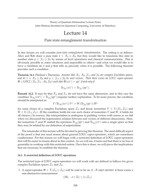
In this lecture we will consider pure-state entanglement transformation.The setting is as follows: Alice and Bob share a pure state x∈X A⊗X B,but they would like to transform this state to another state y∈Y A⊗Y B by means of local operations and classical communication.This is obviously possible in some situations and impossible in others—and what we would like is to have a condition on x and y that tells us precisely when it is possible.The following theorem provides such a condition.Theorem14.1(Nielsen’s Theorem).Assume that X A,X B,Y A,and Y B are complex Euclidean spaces, and let x∈X A⊗X B and y∈Y A⊗Y B be unit vectors.Then there exists an LOCC super-operator Φ∈LOCC(X A,Y A:X B,Y B)such thatΦ(xx∗)=yy∗if and only ifTr XB (xx∗)≺Tr YB(yy∗).Remark14.2.It may be that X A and Y A do not have the same dimension,and in this case thecondition Tr XB (xx∗)≺Tr YB(yy∗)requires further explanation.To be more precise,the conditionshould be interpreted asV(Tr XB (xx∗))V∗≺W(Tr YB(yy∗))W∗for some choice of a complex Euclidean space Z A and linear isometries V∈U(X A,Z A)and W∈U(Y A,Z A).(If the condition holds for one such choice of isometries V and W,it holds for all choices.)In essence,this interpretation is analogous to padding vectors with zeroes as we did when we discussed the majorization relation between real vectors of different dimensions.Here,the isometries V and W embed the operators Tr XB (yy∗)and Tr YB(zz∗)into a single space so thatthey may be related by our definition of majorization.The remainder of this lecture will be devoted to proving this theorem.The most difficult aspect of the proof is that one must reason about general LOCC super-operators,which are sometimes cumbersome.For this reason we will begin with a restricted definition of LOCC super-operators that will be easier to reason about in this context.As we will see,it turns out that there is no loss of generality in working with this restricted notion.Once this is done,we will prove the implications that are necessary to establish the theorem.14.1A restricted definition of LOCC operationsThe restricted type of LOCC super-operators we will work with are defined as follows for given complex Euclidean spaces Z A and Z B.1.A super-operatorΦ∈T(Z A⊗Z B)will be said to be an A→B super-operator if there exists anon-destructive measurement{M a:a∈Σ}⊂L(Z A)108p(a) X+U a Y ∗for each a∈Σ,where X+denotes the Moore–Penrose pseudo-inverse of X(which is discussed in theLecture1notes).For each a∈Σwe haveM∗a M a=p(a)X+U a(YY∗)U∗a(X+)∗,and therefore∑M∗a M a=X+XX∗(X+)∗= X+X X+X ∗=1−Πker(X).a∈ΣSo,{M a:a∈Σ}is not quite a non-destructive measurement,but we can turn it into one by adding an additional element in a similar way that we did in the proof of Theorem14.3—so let us assume0∈Σ,defineΣ′=Σ∪{0},and define M0=Πker(X).Then,{M a:a∈Σ′}is a non-destructive measurement,and therefore so too is its element-wise complex conjugateM a Z U∗a⊗p(a) U∗a XX+U a Y= p(a)Πim(U∗a X)Y=M a(AX)∗W∗a=M a A XW∗aDefiningV a=M a Afor each a∈Σtherefore gives N a XV T a=U a XM T a.It is clear that each V a is unitary and it is easily checked that∑a∈ΣN∗a N a=1ZA,implying that{N a:a∈Σ}is a valid non-destructive measurement.We have therefore proved that for every B→A super-operatorΦ∈T(Z A⊗Z B)and every vector u∈Z A⊗Z B,there exists an A→B super-operatorΨ∈T(Z A⊗Z B)such thatΨ(uu∗)=Φ(uu∗).A symmetric argument shows that for every A→B super-operatorΦand every vector u∈Z A⊗Z B,there exists a B→A super-operatorΨsuch thatΦ(uu∗)=Ψ(uu∗).Finally,notice that the composition of any two A→B super-operators is also an A→B super-operator,and likewise for B→A super-operators.Therefore,by applying the above arguments repeatedly for any given restricted LOCC super-operatorΦand vector u∈Z A⊗Z B,wefind that there exists an A→B super-operatorΨsuch thatΨ(uu∗)=Φ(uu∗),and likewise forΨbeing a B→A super-operator.We are now prepared tofinish the proof.We assume that there exists a restricted LOCC super-operatorΦ∈T(Z A⊗Z B)such thatΦ(xx∗)=yy∗,from which we conclude that there exists a B→A super-operatorΨ∈T(Z A⊗Z B)such thatΨ(xx∗)=yy∗.WriteΨ(Z)=∑a∈Σ(U a⊗M a)Z(U a⊗M a)∗,for{M a:a∈Σ}a non-destructive measurement on Z B and{U a:a∈Σ}a collection of unitary operators on Z A.M a X∗=XX∗. This shows that there exists a mixed unitary super-operatorΞsuch thatXX∗=Ξ(YY∗).which is equivalent toTr ZB (xx∗)=Ξ(Tr ZB(yy∗))as required.。

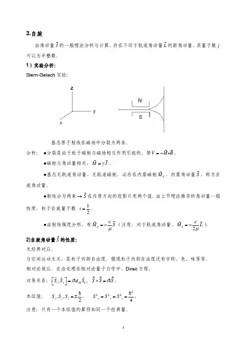
１量 子 力 学 讲 稿(Lecture Notes of Quantum Mechanics)重点参考书目:1.《量子力学》周世勋 1961；2.《量子力学》曾谨言 19823.《量子力学导论》曾谨言 19944.《量子力学》卷I 曾谨言 2000选择参考书目:1.《量子力学》郎道,栗弗席茨 上册 19802.《量子力学》蔡建华 上册 19803.《量子力学》沈仲钧,冯茂仁 19874.《A first course in quantum mechanics》 H. Clark5.《The Principles of Quantum Mechanics》 P. A. M. Dirac (有中译本)第一章 绪 论§1.1经典物理学的困难； §1.2光的波粒二象性§1.3原子结构的玻尔理论；§1.4微粒的波粒二象性第一章 绪 论一、量子力学的研究对象量子力学（Quantum Mechanics）是研究微观实物粒子（静止质量00≠m ）运动变化规律的科学。

二、量子力学在物理学中的地位量子力学在理论理论中占有一个很不平常的地位；它把经典力学作为一种极限形式而包含之，但在它自身表述中，同时又需要这一极限形式。

用方框图表示如下：２三、量子力学的诞生及产生基础1.量子力学的诞生量子力学是1925年诞生的，很快发展成为完整体系，若把旧量子论包括在内，应该说量子力学是1900年12月17日诞生的。

在这一天，德国物理学家Planck 在柏林科学院物理学会的一次会议上，作了有关尝试克服热辐射理论中困难的报告。

2.量子力学产生的基础它产生的基础是光和实物粒子的波粒二象性。

19世纪末、二十世纪初，经典物理学已经发展到了相当完善的阶段。

a.一切物体的低速机械运动规律，准确地遵循Newton 力学规律；b.电磁现象的规律被总结为Maxwell 方程；c.光现象有关的波动理论，最后也被归结为Maxwell 方程；d.热现象有完整的热力学及Boltzman、Gibbs 等人建立的统计力学。

量子力学讲义量子力学的通俗讲座一、粒子和波动我们对粒子和波动的概念来自直接的经验。

和粒子有关的经验对象：小到石子大到天上的星星等；和波动有关的经验对象：最常见的例子是水波，还有拨动的琴弦等。

但这些还不是物理中所说的模型，物理中所谓粒子和波动是理想化的模型，是我们头脑中抽象的对象。

1.1 粒子的图像在经典物理中，粒子的概念可进一步抽象为：大小可忽略不计的具有质量的对象，即所谓质点。

质量在这里是新概念，我们可将其定义为包含物质量的多少，一个西瓜，比西瓜仔的质量大，因为西瓜里包含的物质的量更大。

为叙述的简介，我们现在可把粒子等同于质点。

要描述一个质点的运动状态，我们需要知道其位置和质量（x,m ），这是一个抽象的数学表达。

但我们漏掉了时间，时间也是一个直观的概念，这里我们可把时间描述为一个时钟，我们会发现当指针指到不同位置时，质点的位置可能不同，于是指针的位置就定义了时刻t 。

有了时刻t ，我们对质点的描述就变成了（x,t,m ），由此可定义速度v ，现在我们对质点运动状态的描述是（x,v,t,m ）。

在日常经验中我们还有相互作用或所谓力的概念，我们在地球上拎起不同质量物体时肌肉的紧张程度是不同的，或者说弹簧秤拎起不同质量物体时弹簧的拉伸程度是不同的。

以上我们对质量、时间、力等的定义都是直观的，是可以操作的。

按照以上思路进行研究，最终诞生了牛顿的经典力学。

这里我们可简单地用两个公式：F=ma （牛顿第二定律）和2GMmF x（万有引力公式）来代表牛顿力学。

前者是质点的运动方程，用数学的语言说是一个关于位置x 的二阶微分方程，所以只需要知道初始时刻t=0时的位置x 和速度v 即可求出以后任意时刻t 质点所处的位置，即x(t)，我们称之为轨迹。

需要强调的是一旦我们知道t=0时x 和v 的精确值（没任何误差），x(t)的取值也是精确的，即我们得到是对质点未来演化的精确预测，并且这个求解对t<0也精确成立，这意味着我们还可精确地反演质点的历史。

（完整）量子力学14编辑整理：尊敬的读者朋友们：这里是精品文档编辑中心，本文档内容是由我和我的同事精心编辑整理后发布的，发布之前我们对文中内容进行仔细校对，但是难免会有疏漏的地方，但是任然希望（（完整）量子力学14）的内容能够给您的工作和学习带来便利。

同时也真诚的希望收到您的建议和反馈，这将是我们进步的源泉，前进的动力。

本文可编辑可修改，如果觉得对您有帮助请收藏以便随时查阅，最后祝您生活愉快业绩进步，以下为（完整）量子力学14的全部内容。

§3-6 力学量的平均值按照前面的假设，量子力学中表示力学量的算符为厄米算符,它们的本征函数组成正交归一完备函数系。

比如,力学量算符Fˆ的本征值方程为 )()(ˆx x F nn n ψλψ= 则{}()n x ψ构成正交归一完备本征函数系。

如果量子体系处于状态)(x ψ，则可把它向{}()n x ψ作展开，即∑=ψnn n x c x )()(ψ展开系数⎰ψ=dx x x c n n )()(*ψ如果)(x ψ已归一化，则∑∑∑⎰⎰===ψψ=nn mnmn n m mnn m n m c c c dx c c dx x x 2****)()(1δψψ可以看出，2n c 具有概率的意义，它表示在)(x ψ态下测得ˆF的本征值为n λ的概率。

特别地，如果)(x ψ是算符F ˆ的某一个本征函数()n x ψ,则上式中除21nc =外,其余系数皆为0，此时测量F 时得到的值必为n λ。

因此，力学量F 在)(x ψ态下的平均值为∑=nn n c F 2λ因为∑∑∑⎰∑⎰⎰====ψψnnn mnmn n nm mnn n m n m mnn m n m c c c dxc c dx F c c dx x F x 2******ˆ)(ˆ)(λδλψλψψψ所以,平均值公式又可写成⎰ψψ=dx x Fx F )(ˆ)(* 在三维空间时,平均值公式*ˆ()()F r Fr d τ=ψψ⎰ 例如，在(,)r t ψ态下，坐标的平均值为*(,)(,)r r r t r r t d τ∞-∞==ψψ⎰这一点容易理解，因为2(,)r t d τψ表示t 时刻在r d r r+→内找到粒子的概率,因此2*(,)(,)(,)r r t rd r t r r t d ψτψψτ∞∞-∞-∞==⎰⎰再如，在(,)r t ψ态下，动量的平均值为*ˆ(,)(,)p r t pr t d τ=ψψ⎰ 这一点也可以从动量算符本身推得。