Abstract The Minimum Area Spanning Tree Problem We define and study the Minimum Area Spanni

Using Rewriting-Logic Notation for Funcional Verification in Data-Stream Based Reconfigurable ComputingReiner W. Hartenstein1, Ricardo P. Jacobi2 1Fachbereich Informatik Kaiserslautern University of Technology hartenst@rhhk.uni-kl.de2Depto. De Ciência da ComputaçãoUniversidade de Brasíliarjacobi@cic.unb.br Maurício Ayala-Rincón3, Carlos H. Llanos4 3Departamento de Matemáticaayala@mat.unb.br4Departamento de Engenharia Mecânicallanos@unb.brUniversidade de BrasíliaBrasília - BrazilAbstractReconfigurable Systolic Arrays are a generalization of Systolic Arrays where node operations and interconnections can be redefined even at run time. This flexibility increases the range of systolic array’s application, making the choice of the best systolic architecture to a given problem a critical task. In this work we investigate the specification and verification of such architectures using rewriting-logic, which provides a high level design framework for architectural exploration. In particular, we show how to use ELAN rewriting system to specify reconfigurable systems which can perform both arithmetic and symbolic computations.1. IntroductionThe widespread popularization of mobile computing and wireless communication systems fostered the research on new architectures to efficiently deal with communications issues in hardware constrained platforms like PDAs, mobile phones and pagers, for instance. Some tasks such as data compression, encoding and decoding are better implemented through dedicated hardware modules than using standard general purpose processors (GPP). However, the exploding costs of integrated circuit fabrics associated with shorter devices lifetimes makes the design of ASIC (Application Specific Integrated Circuit) a very expensive alternative. The growing capacity of Field Programmable Gate Arrays (FPGA) and the possibility of reconfiguring them to implement different hardware architectures makes it a good solution to this rapid changing wireless market. An FPGA may be configured to implement a cipher algorithm at one moment and can be later reconfigured to implement a data compressing algorithm. This flexibility opens a wide range of architectural alternatives to implement algorithms directly in hardware. In this context, it is very important to provide methods and tools to rapidly model and evaluate different hardware architectures to implement a given algorithm.In this paper we propose the use of rewriting systems to model and evaluate reconfigurable systolic hardware architectures. After the seminal work of Knuth-Bendix about the completion of algebraic equational specifications, which allows for the automatic generation of a rewrite-based theorem prover for the equational reduct of the subjacent treated theories [KnBe70], rewriting has been successfully applied into different areas of research in computer science as an abstract formalism for assisting the simulation, verification and deduction of complex computational objects and processes. In particular, in the context of computer architectures, rewriting theory has been applied as a tool for reasoning about hardware design.To review only a reduced set of different approaches in this direction, we find of great interest the work of Kapur who has used his well-known Rewriting Rule Laboratory - RRL(the first successful prover assistant based on rewriting) for verifying arithmetic circuits [KaSu2000, Ka2000, KaSu1997] as well as Arvind’s group that treated the implementation of processors with simple architectures [ShAr98a,ShAr98b,ArSh99], the rewrite-based description and synthesis of simple logical digital circuits [HoAr99] and the description of cache protocols over memory systems [RuShAr99,ArStSh01]. Also contributions in this field have shown how rewriting theory can be applied for the specification of processors (as Arvind’s group does) as well as for the purely rewrite based simulation and analysis of the specified processors [ANJLH02]. To achieve this rewriting-logic has been applied, that extends the pure rewriting paradigm allowing for a logical control of the application of the rewriting rules bystrategies [Me00,CiKi99]. Important programming environments based on the rewriting-logic paradigm are ELAN [CiKi99,BKKM02], Maude [Me00,Cla02] and Cafe-OBJ [DiFu02]. The impact of rewriting-logic as a successful programming paradigm in computer science as well as of the applicability of the related programming environments is witnessed by [MOMe02]. All our implementations and experiments were done in ELAN, since we consider of great flexibility its easy manipulation of strategies. However, for effects of model checking Maude has been proved to be more adequate.Section 2 provides an introduction to basic concepts in rewriting theory and reconfigurable circuits. Section 3 presents the specification and simulation of reconfigurable systolic arrays. Section 4 discusses use of rewriting-logic for simulating reconfiguration and another approach for data driven systolic arrays and section 5 is the conclusion.2. BackgroundAn example of our typical target environments is mapping applications onto platforms like coarse-grained DPAs (DataPath Arrays) or rDPAs (reconfigurable DPAs). We assume, that such platforms are completely pre-debugged, so that only the related mapping source has to be verified. Using Term Rewriting Systems (s. section 2.1) in such an environment means to specify or verify designs from sources at abstraction levels being higher than that of languages like VHDL or Verilog. Such notations are much more compact and concise than with traditional hardware language source notations in EDA. An example is the input language of ELAN which is a parsable derivative of the math formula space.This paper uses systolic arrays as demo examples (section 2.2). Systolic arrays, however, are special cases of super-systolic platforms like DPAs or rDPAs [HaKrRe95], which are data-stream-based [Ha03] pipe networks. (By the way: such platforms may also be emulated on larger FPGAs.) The only difference between systolic and super-systolic is the mapping method [Ha97]. Algebraic mapping or linear projection methods yield only solutions with linear uniform pipes which is restricted to the special case of applications with strictly regular data dependencies. But using simulated annealing, genetic algorithms or other optimization methods, permits any heterogeneous networks with free form pipes like zigzag, circular, or any much more wild shapes, and may also include forks and joins. The methodology introduced by this paper may be used for all kinds of data-stream-based hardwired or reconfigurable platforms.2.1. Rewriting theoryWe include the minimal needed notions on rewriting theory and rewriting-logic. For a detailed presentation of rewriting see [BaNi98].A Term Rewriting System, TRS for short, is defined as a triple ·R, S, S0 Ò, where S and R are respectively sets of terms and of rewrite rules of the form l ’ r i f p(l)being l and r terms and p a predicate and where S0 is the subset of initial terms of S. l and r are called the left-hand and right-hand sides of the rule and p its condition.In the architectural context of [ShAr98b], terms and rules represent states and state transitions, respectively.A term s can be rewritten or reduced to the term t, denoted by s ’ t, whenever there exists a subterm s' of s that can be transformed according to some rewrite rule into the term s'' such that replacing the occurrence of s' in s with s'' gives t. A term that cannot be rewritten is said to be in normal or canonical form. The relation over S given by the previous rewrite mechanism is called the rewrite relation of R and is denoted by ’. Its inverse is denoted by ¨and its reflexive-transitive closure by ’*and its equivalence closure by ´*.The important notions of terminating property (or Noetherianity) and Church-Rosser property or confluence are defined as usual. These notions correspond to the practical computational aspects as the determinism of processes and their finiteness.•a TRS is said to be terminating if there are no infinite sequences of the form s0’ s1’ ...• a TRS is said to be confluent if for all divergence of the form s ’* t 1, s ’* t 2 there exists a term u such that t 1 ’* u and t 2 ’* u .The use of the subset of initial terms S 0, representing possible initial states in the architectural context (which is not standard in rewriting theory), is simply to define what is a "legal" state according to the set of rewrite rules R ; i.e., t is a legal term (or state) whenever there exists an initial state s Œ S 0 such that s ’* t .Using these notions of rewriting one can model the operational semantics of algebraic operators and functions. Although in the pure rewriting context rules are applied in a truly non deterministic manner in the practice it is necessary to have a control of the ordering in which rules are applied. Thus rewriting theory jointly with logic, that is known as rewriting-logic, has been showed of practical applicability in this context of specification of processors since they may be adapted for representing in the necessary detail many hardware elements involved in processors. Moreover, other important fields of hardware design such as verification and synthesis of logical circuits may be benefited from the simplicity and versatility of this theoretical framework.2.2. Systolic arrays and reconfigurable systemsA systolic array is a mesh-connected pipe network of DPUs (datapath units), using only nearest neighbor (NN) interconnect [Ku78, Ku87]. DPU functional units operate synchronously, processing streams of data that traverse the network. Systolic arrays provide a large amount of parallelism and are well adapted to a restrict set of computational problems, i.e., those which can be efficiently mapped to a regular network of operators.Figure 1 shows a simple systolic example of a matrix-vector multiplication. The vector elements are stored inthe cells and are multiplied by the matrix elements thatare shifted bottom-up. On the first cycle, the first cell(DPU1) computes x 1*a 11, while the second and third cells(DPU2 and DPU3) multiply their values by 0. On thesecond cycle, the first cell computes x 1*a 21, while thesecond cell computes x 1*a 11 + x 2*a 12, where the first termis taken from the first cell and added to the productproduced in second cell. In the third cycle, the third cellproduces the first result : y 1 = x 1*a 11 + x 2*a 12 + x 3*a 13. Inthe following two cycles y 2 and y 3 will be output by thethird cell.There are several alternative configurations of functional cells, each one tailored to a particular class of computing problems. However, one of the main critics to systolic arrays is its restriction to applications with strictly regular data dependencies, as well as its lack of flexibility. Once designed, it is suitable to support only one particular application problem.The limitations of systolic arrays may be circumvented by using reconfigurable circuits, the most representative of them being the FPGAs (Field Programmable Gate Arrays). An FPGA can have its behavior redefined in such a way that it can implement completely different digital systems on the same chip. Fine grain FPGAs may redefine a circuit at the gate level, working with bit wide operators. This kind of architecture provides a lot of flexibility, but takes more time to reconfigure than coarse grain reconfigurable platforms (rDPAs: reconfigurable DPAs). These work with word wide operators that are slightly less flexible but more area efficient and take much less time to reconfigure than the fine grain ones. The design of reconfigurable systolic architectures [HaKrRe95, HHHN00] aims to overcome the restriction of pure systolic circuits while keeping the benefits of a large degree of parallelism. In the reconfigurable approach, the operations performed by each functional unit as well as the interconnection among them may be reconfigured in order to be adapted to different applications. Moreover, it is possible to change the configuration of the circuit during run time, an approach called dynamic reconfiguration, which broadens even more the architectural alternatives to implement applications in hardware.a 21a 31a 12a 22a 32a 13a 23a 330y 1 = a 11x 1+a 12x 2+a 13x 3y 2 = a 21x 1+a 22x 2+a 23x 3y 3 = a 31x 1+a 32x 2+a 33x 3Figure 1: Vector – matrix computation.3. Specification and Simulation of Systolic Arrays via Rewriting-LogicHere we show how rewriting-logic can be applied to specify simple systolic arrays for vector andmatrix multiplication using the ELAN system. In these systems we can consider as the reconfigurablepart the constants in each component (DPU as in Figure 1), here called MAC (Multiplier/Adder).Vector multiplication: ELAN provides a very flexible programming environment where the user defines the syntax and semantics of data types (called sorts) and operations to be used in the program.Figure 2 shows the syntax of the data types in the ELAN program that models the vector multiplication.In the left side of a definition the data is specified using a combination of text and place holders which are represented by an ‘@’ character. For instance, an element of sort Port is defined as port(@, @). Thesort of the parameters as well as the sort of the element itself is defined in the right side of the definition.In this example, the two parameters of port are an integer and a Boolean, and the resulting element port(int, bool) is of sort Port. A MAC data is composed of six elements. The sort of the elements is, respectively, int, for the identifier, two of sort Port and two of sort Reg for the ports and registers andone of sort Const for the respective constant component of the multiplier vector. The processor sort Procconsists of four components: three of sort MAC and one of sort DataStream. The DataStream isdescribed as an object with three components of sort list[Data].operators global@ : ( int ) Const;port(@,@): ( int bool ) Port;reg(@,@): ( int bool ) Reg;'[' @,@,@,@,@,@ ']': ( int Port Port Reg Reg Const ) MAC;'<' @ @ @ @ '>' : ( MAC MAC MAC DataStream ) Proc;( @ @ @ ): ( list[Data] list[Data] list[Data] ) DataStream;@: ( int ) Data;endFigure 2. Sorts of the MAC in ELANThe rule named sole, used to describe the behavior of the processor during each cycle of the execution is given in figure 4. Informally, the rule is fired when the expression being processed matches the left side of the rule. It is replaced by the expression produced at the right side of the rule, which is again matched against the set of rules that define the program. Rules can be named for future reference when defining strategies. The rule name sole appears between square brackets in the beginning of the rule. Observe that after one-step of reduction applying this rule all necessary changes in the specified processor are executed. First, notice that the data d1, d2 and d3 at the top of the DataStream, are removed from the three lists of data and placed in the first ports of the three MACs.Figure 3. MAC Systolic Array ArchitectureThe multiplications between the contents of each first port vpi1 and the corresponding constant c i are placed in the first register of each MAC, for i=1,2 3 and 3 and the additions between the first register vri1 and the second port vpi2 are placed in the second port of each MAC, for i=1,2 and 3. Zeros preceding each operator v i are included to synchronize the two operations executed in each MAC. Finally, observe the data transfer from the second register vri2 of each MAC to the second port of the next component vp(i+1)2for i=1 and 2. All that is simultaneously done by only one application of the rewriting rule sole.With respect to the timing aspects of this example, the model assumes a clocked operation like traditional systolic architectures. There is no handshake between nodes and each application of rule sole corresponds to a single clock cycle. Thus, each node in fig. 3 takes two clock cycles to produce itsoutput. The synchronization between nodes for the first values is achieved introducing pairs of zero values, as illustrated in figure 3, and the Boolean flags used to synchronize nodes could be omitted.Executing all steps with a singe rewriting rule could appear artificial in other contexts of computer science, such as semantics of programming languages and in general theory of computing. Nice but relatively complex theoretical results can be related with the possibility of having a unique rewriting rule which simulates a (universal) Turing machine [Da1989, Da1992]. This nontrivial theoretical development may be better understood when we relate a sole rule with the execution of a "cycle" of a processor.rules for Procd1,d2,d3 : int; // variables for input datal1,l2,l3 : list[Data]; // lists of input datavp11, vp12, vp21, vp22, vp31, vp32 : int; // portsvr11, vr12, vr21, vr22, vr31, vr32 : int; // registersc1, c2, c3 : int; // constantsglobal[sole]<[1,port(vp11,true),port(0,true),reg(vr11,true),reg(vr12,true),c1][2,port(vp21,true),port(vp22,true),reg(vr21,true),reg(vr22,true),c2][3,port(vp31,true),port(vp32,true),reg(vr31,true),reg(vr32,true),c3 ](d1.l1 d2.l2 d3.l3) > =><[1, port(d1,true),port(0,true),reg(vp11*c1,true), reg(0+vr11,true),c1 ][2, port(d2,true),port(vr12,true),reg(vp21*c2,true), reg(vp22+vr21,true),c2 ][3, port(d3,true),port(vr22,true),reg(vp31*c3,true), reg(vp32+vr31,true),c3 ](l1 l2 l3) >endendFigure 4. ELAN Description of the Sole Rule.For our example we will consider as simple mechanism of reconfiguration the possibility of changing the constants in each MAC. Then a computation with our systolic array consists of two stages: a reconfiguration stage, where the constants are set and the subsequent processor execution with the previously defined rule sole.Figure 5 shows one additional rule created for the reconfiguration of a processor called conf. It simply changes the contents of the constant part of each MAC(in our case by the vector (1,0,0)). Observe that with the pure rewriting based paradigm this rule applies infinitely, because the resulting expression will match against the left side of the rule again and again. Thus, for controlling its application, we define a logical strategy, called withconf.withconf simply allows for the execution of one-step of reduction with the rule conf(the first reconfiguration stage) and a subsequent normalization with the rule sole (the second processor execution stage). This normalization is an available ELAN strategy, which applies the rewriting rules given as argument (in our case the rule sole) until a normal form is reached.[conf]< [1,port(vp11,true),port(0,true),reg(vr11,true),reg(vr12,true),c1][2,port(vp21,true),port(vp22,true),reg(vr21,true),reg(vr22,true),c2][3,port(vp31,true),port(vp32,true),reg(vr31,true),reg(vr32,true),c3](d1.l1 d2.l2 d3.l3) > =>< [1,port(vp11,true),port(0,true),reg(vr11,true),reg(vr12,true),1][2,port(vp21,true),port(vp22,true),reg(vr21,true),reg(vr22,true),0][3,port(vp31,true),port(vp32,true),reg(vr31,true),reg(vr32,true),0](d1.l1 d2.l2 d3.l3) >endstrategies for Procimplicit[] withconf => conf; normalise(sole) end[] simple => normalise(sole) endendFigure 5. conf Rule for ReconfigurationMatrix Multiplication:figure 6 shows the matriz multiplication structure and the description of its components is given in figure 7. Using the previous approach (that is, specifying a sole rule) implies the use of an excessive number of variables, which is not directly supported in ELAN. In fact, we would need different variables for the two ports, three registers and the constant belonging to each MAC, whichgives a total of 96 variables; additionally, we would need 16 variables for describing the two 4x data streams. This could be done by enlarging the ELAN capacity for dealing with variables before compiling the system. But a better solution is to split the cycle defining independent rewriting rules to be applied under a reasonable strategy, to simulate the internal process into each MAC component and the propagation of data between each component to their North and East connected MAC s.We define a rule for each of the sixteen components, which propagates the contents into their registers two and three to their North and East connected components, respectively. As a consequence of the form in which data should be transferred in the processor, these sixteen rules should be applied from the right to the left and top-down in order to complete a whole cycle of execution.Figure 6. Systolic Matrix-vector multiplicationoperators global@ : ( int ) Const;p(@) : ( int ) Port;r(@) : ( int ) Reg;'['@,@,@,@,@,@,@']' : ( int Port Port Reg Reg Reg Const ) MAC;'<' @@ @ @ @@ @ @ @@ @ @ @@ @ @ @@ '>: ( DataStringMAC MAC MAC MAC // MACs 13 14 15 16MAC MAC MAC MAC // MACs 09 10 11 11MAC MAC MAC MAC // MACs 05 06 07 08MAC MAC MAC MAC // MACs 01 02 03 04DataString ) Proc;( @ @ @ @ ) : ( list[Data] list[Data] list[Data] list[Data] )DataString;@ : ( int ) Data;endFigure 7. A 4¥4 Systolic array DescriptionAll these rules are very similar and a selected group of them is presented in the Figure 8. The rules for the South (mac01, mac02, mac03, mac04) and West (mac01, mac05, mac09, mac13) MAC s, called boundary components of the processor, load the data (dS and dW) in the head of the corresponding list of the data stream (lS1, lS2, lS3, lS4 and lW1, lW2, lW3 and lW4). Moreover, the rules for MAC s in the North (mac13, mac14, mac15, mac16) and East (mac04, mac08, mac12, mac16) boundaries of the processor only transfer data to the East and North corresponding boundary components; except, of course, for mac16. Consequently, different orderings for applying these rules completing a whole cycle of the processor are possible. For instance, we could take the ordering: mac16, mac12, mac08, mac04, mac15, mac11, mac07, mac03, mac14, mac13, mac10, mac09, mac06, mac05, mac02, mac01.In the Figure 9 we present a possible strategy called onecycle which defines an(other) ordering of application of these rules for completing a sole cycle of the processor. For completing the simulation of execution with this simple processor, one should define a normalization via this strategy: normalise(onecycle). In this rewriting-logical environment, our specification could be easily modified allowing the interpretation of parts of the processors as reconfigurable components.At first glance, one could look at the constants of the 16 MAC s as a reconfigurable component. In this way the processor can be adapted to be either a 4-vector versus 4x4-matrix multiplier or vice-versa and the 4x4-matrix may be modified to represent, for example, either the identity or the matrix F 4 of the Fast Discrete Fourier Transform (FFT).rules for Proc m01,m02,m03,m04,m05,m06,m07,m08: MAC; // 1-8 MACs m09,m10,m11,m12,m13,m14,m15,m16:MAC; //9-16 MACs dW, dS : int; // data East and SouthlW1,lW2,lW3,lW4,lS1,lS2,lS3,lS4:list[Data]; // West andSouthr1,r2, r3,rN1,rN2,rN3 : int; // Central North andrE1,rE2,rE3 : int; // East registers 1,2,3p1,p2,pN1,pN2,pE1,pE2: int; //Central,North and East portsc,cE,cN : int;global[mac16]< (lW1 lW2 lW3 lW4)m13 m14 m15 [16,p(p1),p(p2),r(r1),r(r2),r(r3),c ]m09 m10 m11 m12m05 m06 m07 m08m01 m02 m03 m04(lS1 lS2 lS3 lS4) > =>< (lW1 lW2 lW3 lW4)m13 m14 m15 [16,p(p1),p(p2),r(p1*c),r(r1+p2),r(p1),c ]m09 m10 m11 m12m05 m06 m07 m08m01 m02 m03 m04(lS1 lS2 lS3 lS4) >end ...[mac11]< (lW1 lW2 lW3 lW4)m13 m14 [15,p(pN1),p(pN2),r(rN1),r(rN2),r(rN3),cN ] m16m09 m10 [11,p(p1),p(p2),r(r1),r(r2),r(r3),c ][12,p(pE1),p(pE2),r(rE1),r(rE2),r(rE3),cE ]m05 m06 m07 m08m01 m02 m03 m04(lS1 lS2 lS3 lS4) > =>< (lW1 lW2 lW3 lW4) m13 m14 [15,p(pN1),p(r2),r(rN1),r(rN2),r(rN3),cN ] m16 m09 m10 [11,p(p1),p(p2),r(p1*c),r(r1+p2),r(p1),c ] [12,p(r3),p(pE2),r(rE1),r(rE2),r(rE3),cE ] m05 m06 m07 m08 m01 m02 m03 m04 (lS1 lS2 lS3 lS4) >end ...…… [mac01]< (dW.lW1 lW2 lW3 lW4) m13 m14 m15 m16 m09 m10 m11 m12 [05,p(pN1),p(pN2),r(rN1),r(rN2),r(rN3),cN ] m06 m07 m08 [01,p(p1),p(p2),r(r1),r(r2),r(r3),c ] [02, p(pE1),p(pE2),r(rE1),r(rE2),r(rE3),cE]m03 m04 (dS.IS1) IS2 IS3 IS$) > =>< (IE1 IE2 IE3 IE4) m13 m14 m15 m16 m09 m10 m11 m12 [05, p(pN1),p(r2) r(rN1) r(rN2) r(rN3), cN] m06 m07 m08 [01, p(dW), p(dS),r(p1*c), r((rE2), r(rE3), cE] m03 m04 (IS1 IS2 IS3 IS4)>end end Figure 8. A selected set of rules for matrix-vector multiplipy.Strategies for Procimplicit[] onecycle =>mac16;mac15;mac14;mac13;mac12;mac11;mac10;mac09;mac08;mac07;mac06;mac05;mac04;mac03;mac02;mac01 end end Figure 9. onecycle strategy for rule application.reconfF4 => F4;normalise(mac16;mac15;mac14;mac13; mac12;mac11;mac10;mac09; mac08;mac07;mac06;mac05; mac04;mac03;mac02;mac01)endFigure 10: strategy working over processor.The last is specified by a strategy additional, that is presented at the Figure 11, which before to the simulation of the normalization executes the rewrite rule F 4. F 4 transforms any given state of the processor into another where the reconfigurable constants are replaced with the corresponding powers of a primitive complex 4-root of the unity of F 4 (either i o r -i ) as illustrated in the Figure 11. In this specification the components of each MAC have been divided into the fixed ones and the reconfigurable constant [fxnn cnn]. This simple idea can be directly extended to different kind of MAC s , where other components are considered to be reconfigurable.[F4]< dstreamEast[fx13 c13] [fx14 c14] [fx15 c15] [fx16 c16][fx09 c09] [fx10 c10] [fx11 c11] [fx12 c12][fx05 c05] [fx06 c06] [fx07 c07] [fx08 c08][fx01 c01] [fx02 c02] [fx03 c03] [fx04 c04]dstreamSouth > =>< dstreamEast [fx13 i 0] [fx14 i 3] [fx15 i 6] [fx16 i 9] [fx09 i 0] [fx10 i 2] [fx11 i 4] [fx12 i 6] [fx05 i 0] [fx06 i 1] [fx07 i 2] [fx08 i 3] [fx01 i 0] [fx02 i 0] [fx03 i 0] [fx04 i 0]dstreamSouth >endFigure 11: rule for FFT Transformer4. Alternative Models4.1 Variable Size Systolic ArraysOne limitation of the ELAN models presented aboveis that the rules are defined for a specific systolicarchitecture. A more flexible description will allow thespecification of systolic arrays with an arbitrary numberof functional units. In this case, the rewriting rulesshould be defined independently of the array size ortopology.This is exemplified in this section through the modeling of a simple version of the KressArray architecture [HaKrHe95]. It is defined by a matrix of reconfigurable functional units (rDPUs: reconfigurabledatapath units) where both the operations and the interconnections may be redefined (compare fig. 12 c and d). Figure 12 illustrates a KressArray family design space, which covers a wide variety of reconfigurable connect fabrics: nearest neighbour interconnect (NN) and backbus fabrics (segmented and / or non-segmented). Figure 13 shows a detailed example of NN ports featuring individual path width and individual mode (in, out, or bi-directional).Mapping C expressions to KressArrays is performed by assigning C operators to the nodeswhile keeping the corresponding data dependency among them. One particularity is that a KressArray is a pipe network which implements a dataflow model of computation. Coming along with synthesis tools also supporting non-uniform non-regular pipe networks [HHHN00, Na01] (in contrast to classical systolic array synthesis methods accepting only applications with strictly regular data dependencies) the KressArray family is a generalization of the systolic array. In addition to the generalized NN interconnect the KressArray family also provides abackbus (BB) second level interconnect fabrics with resources like buses and bus segments (for familymember examples see fig. 12 e, f, g).The DPU nodes of both, systolic arrays and rDPAs,may operate in a clocked mode, or asynchronously,where each operation is triggered as soon as data isavailable at the node inputs. (The latter version ofsystolic arrays has been usually called wavefrontarrays). This asynchronous operation is accomplishedby a handshake between interconnected nodes, sinceeach operation may take several clock cycles(multiplication, for instance, is implemented in itstypical serial way, through sums and shifts).Modeling of KressArrays in ELAN takes a different approach. To allow the specification of variable size systolic arrays, the nodes are stored on a list of arbitrary length. The designer provides the interconnections among nodes through signals, implemented with variables that connect the registers at the inputs and outputs of the nodes. Thus, if node n i is connected to node n j , then the same variable is associated to n i output and n j input. The operations of the nodes are dynamically specified along with the data that is to be processed by the array. To illustrate this kind of modeling lets consider a practical example: a KressArray that computes the differential equation loop body, given in figure 14.This array is defined by a list of 12 nodes, numbered from left to right and top to bottom. The first 4nodes are presented in figure 15. Each rDPU node is a kind of rAlu (reconfigurable Arithmetic-Logic Unit). In this simplified version, each rDPU has two registers in the inputs and one register at the output.Each register is defined by the variable it holds, its value and a flag that indicates if the data it holds is valid. The flag models the signal used for handshake in hardware. Rule assign() is used by the designer to provide values to input variables, specified in the form “x=5.y=2…”. Then, rule dpu() is applied to the Figure 12. KressArray family design space:(a, b) NN fabrics examples; (e, f, g) backbus (BB) fabrics examples; rDPU configuration:c) routing only configuration, d) routing and function configuration Figure 13: a KressArray family member example illustrating individual port mode and path width。

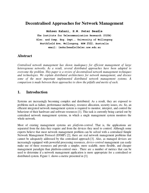
Decentralised Approaches for Network ManagementMohsen Kahani, H.W. Peter BeadleThe Institute for Telecommunication Research (TITR)Elec. and Comp. Eng. Dept., University of WollongongNorthfield Ave, Wollongong, NSW 2522, Australiaemail: {moka|beadle}@.auAbstractCentralised network management has shown inadequacy for efficient management of large heterogenous networks. As a result, several distributed approaches have been adapted to overcome the problem. This paper is a review of decentralised network management techniques and technologies. We explain distributed architectures for network management, and discuss some of the most important implemented distributed network management systems. A comparison is made between these approaches to show the pitfalls and merits of each.1.IntroductionSystems are increasingly becoming complex and distributed. As a result, they are exposed to problems such as failure, performance inefficiency, resource allocation, security issues, etc. So, an efficient integrated network management system is required to monitor, interpret, and control the behaviour of their hardware and software resources [1]. This task is currently being carried out by centralised network management systems, in which a single management system monitors the whole network.Most of existing management systems are platform-centred. That is, the applications are separated from the data they require and from the devices they need to control. Although some experts believe that most network management problem can be solved with a centralised Simple Network Management Protocol (SNMP) [2], there are real network management problems that cannot be adequately addressed by this centralised approach [3]. Also, as managed devices are increasingly equipped with powerful processing resources, device-centred management can easily make use of these resources and provide a simpler, more scalable, more flexible, and cheaper management paradigm than platform-centred ones . There are a number of metrics that can be used to determine if a network management application is more appropriate for a centralised or distributed system. Figure 1. shows a metric presented in [3].Figure 1. Metrics to determine decentralisationIn this paper, we focus on non-centralised approaches for network management, and discus several architectures proposed to accomplish this purpose. We initially, explain different architectures for network management systems. Then, we present background information on distributed systems and then discuss several implemented distributed network management systems. Finally, we will conclude the paper with a comparison between these systems and discuss their pitfalls and merits.work Management ArchitecturesThere are three basic approaches for network management systems: centralised, hierarchical and distributed [4]. Currently, most network management systems are centralised. That is, there is a single management machine which collects the information and controls the entire network (Figure 2.-a). This workstation is a single point of failure, and if it fails, the entire network could collapse. In case the management host does not fail, but a fault partitions the network, the other part of the network is left without any management functionality. Also, a centralised system cannot easily be scaled up when the size or complexity of the network increase [5].A variation of centralised systems is the platform approach [6] (Figure 2.-b), in which a single manager is divided into two parts: the management platform and the management application. The management platform is mainly concerned with information gathering and simple calculations, while management application uses the services offered by the management platform to handle decision support and higher functions [7]. The advantage of this approach is that applications do not need to worry about protocol complexity and heterogeneity. The drawback is that it still inherits limited scalibility from its centralised architecture.The hierarchical architecture uses the concept of “Manager of Managers” (MOM) and manager per domain paradigm[4, 6] (Figure 2.-c). Each domain manager is only responsible for the management of its domain, and is unaware of other domains. The manager of managers sits at a higher level and request information from domain managers. In this architecture, there is no directcommunication between domain managers. This architecture is quite scalable, and by adding another level of MOM a multiple level hierarchy can be achieved.The distributed approach (Figure 2.-d) is a peer-to-peer architecture[4]. Multiple managers, each responsible for a domain, communicate with each other in a peer-system. Whenever information from another domain is required, the corresponding manager is contacted and the information is retrieved. By distributing management over several workstations throughout the network, the network management reliability, robustness and performance increases, while the network management costs in communication and computation decrease [5]. This approach has also been adapted by ISO standards and the Telecommunication Management Network (TMN)architecture [8]. The Management model for ATM networks, adapted by ATM Forum, is based on this approach, too [9].A combination of the hierarchical and distributed architectures, known as ‘network architecture’,can also be used [6] (Figure 3.). This architecture uses both manager-per-domain and manager of managers concepts, but instead of a purely peer-system or hierarchical structure, the managers are organised in a network scheme. This approach preserves the scalibility of both systems and provides better functionality in diverse environments.ManagementWorkstation Network Agent Agent Agent (a)(Multiple-vendor)NetworkAgent Agent Agent(b)Management PlatformApplication Application (Multiple-protocol)Network Agent Agent Agent(c)Manager 1Manager n domain 1domain n Manager of Managers(MOM)NetworkAgent Agent Agent (d)Manager 1Manager n domain 1domain nFigure 2. Different management approaches: a) Centralised, b) Centralised Platform-based,c) Hierarchical and d) Distributed.Integrated Manager 1IntegratedManager 3 IntegratedManager 2Element Manager 1ElementManager 2ElementManager n Networkdomain 1domain nFigure 3. Network Architecture3.Distributed Systems and ServicesFault tolerance and parallelism are key properties of a distributed system [10]. A distributed system should use interconnected and independent processing elements to avoid having a single point of failure. There are also several other reasons why a distributed system should be used. Firstly, higher performance/cost ratio can be achieved with distributed systems. Also, they achieve better modularity, greater expansibility and scalibility, and higher availability and reliability [11]. Distribution of services should be transparent to users, so that they cannot distinguish between a local or remote service. This requires the system be consistent, secure, fault tolerant and have a bounded response time. The form of communication in such systems is referred to as client/server communication [12]. The client/server model is a request-reply communication that can be: synchronous and blocking, in which the client waits until it receives the reply; or asynchronous and non-blocking, in which the client can manage to receive the reply later.Remote Procedure Call (RPC) [13, 14] is well-understood control mechanism used for calling a remote procedure in a client/server environment. The idea is to extend the use of procedure call in local environment to distributed systems. This results in simple, familiar and general methods that can be implemented efficiently.The Object Management Group’s (OMG) Common Object Request Broker Architecture (CORBA) [15] is also an important standard for distributed object-oriented systems. It is aimed at the management of objects in distributed heterogenous systems. CORBA addresses two challenges in developing distributed systems: making the design of a distributed system not more difficult than a centralised one; and providing an infrastructure to integrate application components into a distributed system [16].4.Non-centralised Network ManagementIn this section, we will discuss some of the most important proposed systems for management of networks using non-centralised approaches. These systems include distributed big brother, from the University of Michigan; Distributed Management Environment, from the Open Software Foundation (OSF); hierarchical network management, from the Technical University of Vienna (TU-Wien); and management by delegation, from the University of Columbia. A comparison will be presented in the next section. There are several other approaches, which are not discussed in this paper. Interested readers can refer to [17-24].4.1.Distributed Big BrotherDistributed Big Brother (DBB) is a distributed network management system consisting of cooperative autonomous computing agents [5]. DBB has been designed with the goal of distributing management and organisational tasks, while maintaining a central location control over the whole system. It uses some technologies from the field of distributed AI, such as contracting information, organisational structuring, election for role management, and hierarchical control.DBB distributes the management tasks by using mid-level managers that can be executed in parallel. It also uses the Contract Net Protocol [25] to reduce the overhead in authority structure. As the computer networks changes dynamically, it is not desirable to distribute the tasks only at time of initialisation. So, DBB allows the system to undergo an organisational self-design [26], and changes the submanagers roles as the network structure varies.In DBB each agent consists of three basic functional modules: the communication process, the contracting process, and the task process. The communication process continuously checks whether a message has been sent to the agent, and if so, transmit it to the contracting process, which parses them and does appropriate actions. Finally, the task process carries out the agent’s management task.Agents' roles are not static. An agent does not have any management role as it enters the network. At the time of initialisation, or whenever required, the agents choose a chairman to elect the LAN manager. The chairman announces the election and selects the best nominate (eg. least busy host) and broadcasts its decision. After electing the LAN manager, all other agents become group managers and execute tasks for information gathering. The LAN manager, which is responsible for managing the whole LAN, uses contracting to assign tasks to group managers. Finally, there is a fixed top manager, which uses contracting to request reports from LAN managers.A network can have an arbitrary number of LAN managers and group managers. As LAN managers have some sort of autonomy and independency, more LAN manager means more autonomous and independent network management systems, which corresponds to higher robustness. Increasing the number of group managers increases the number of polling agents, which corresponds to a more frequent polling and more updated management information. However, there is trade off between increasing number of LAN and group managers and extratraffic caused by communication between top manager and LAN managers, and between each LAN manager and its group managers.4.2.Distributed Management Environment (DME)The Open Software Foundation’s (OSF) Distributed Management Environment (DME) is an attempt to represent a structure under which the management of systems and networks can be brought together [27]. It tries to provide a standard set of services to bring management to everything, from bridges and router to server-based operating systems and applications [28].DME is operating system-independent and supports several standards, such as SNMP and CMIP.DME is tailored to OSF Distributed Computing Environment (DCE) [29]. DCE is a comprehensive and integrated service that allows development, distribution and maintenance of distributed applications. It masks the physical complexity of the networked environment and provides a layer of logical simplicity. DCE uses RPC for communication and provides distributed directory services, security services, time services and thread services. Using services provided by DCE, DME provides manageability and allows network components and applications to be well maintained.DME consists of a framework that provides the building blocks for application development and some of the most critical system management functions, such as software management, licence management and printing services. The architecture of the DME allows the addition of new services. It consists of two key components: Manager Request Broker (MRB) and Object Server,as shown in Figure 4.The MRBs are central pieces in the DME framework; they implement the basic APIs that access the services furnished by the DME. The MRB establishes a standardised programming interface to SNMP and CMIP, known as Consolidated Management API (CM-API). The MRB also provides ObjectServer ObjectServer ManagementRequestBroker (MRB)Management Request Broker (MRB)Management Protocol SNMP/CMIPSNMP/CMIP AgentAgentManagementApplication Management ApplicationManagementApplication Object Server Figure 4. DME in detailsa way for management applications to invoke one of the methods associated with a DME object.The object server provides access to the data stored in the object and can create or delete instances of an object. Whenever the MRB receives a message, it sends it to an object server that is associated with the target object. The MRB finds the object by using the Distributed Computing Environment (DCE) directory services.The major problem of DME is that, if all network management platform vendors adapt their system to the DME framework, there will be no differentiating features [30]. As a result platform vendors haven’t attempted to conform to the it, and although DCE gained success and popularity in the market, DME has not.4.3Hierarchical Network ManagementHierarchical network management system [31] uses the concept of SubManager, similar to the manager-to-manager(M2M) protocol described in SNMPv2[32]. A SubManager is associated with a few agents, and collects the primitive information from them, performs some calculations,and produces more meaningful values that can be used by a superior manager. This method significantly reduces the amount of management traffics, because only high-level information is sent to the master manager.Whenever network operators need more, or high-level, information a downloaded Network Management Procedure (NMP) is dynamically assigned to the system. This allows dynamic reconfiguration at run-time, and removes the need to hard-wire everything at compile time [31].The NMPs are loaded into submanagers, and are stored in two tables: subMgrEntry and subMgrOps . Each procedure is Periodically activated and a “Worker” is created, which subMgrValue subMgrOpsControllersubMgr subMgr WorkerWorker AgentSubManager Manager Network ManagementProcedure (NMP)Presentationof resultget/response (SNMPv1/v2)subMgrEntry Create WorkerFigure 5. Internals of the SubManagerevaluates the procedure and stores the result into subMgrValue table This table is read by the manager. This procedure is illustrated in Figure 5.4.4.Management by Delegation (MbD)Most distributed management systems use a traditional client/server process interaction method, such as Remote Procedure Call (RPC). The current implementation of this architecture lacks the required flexibility and needs recompilation and reinstallation of the application whenever a modification is made [1]. Management by Delegation (MbD) [33, 34, 35] is a more flexible paradigm and uses the concept of elastic server [36], whose functionality can be extended at execution time by delegating new functional procedures to it.In MbD, instead of bringing a device’s data to the management platform application, applications are delegated to devices and executed in the same environment that data exists. The delegator entity (manager) uses a delegation protocol to download and control a delegated program (DP). An elastic server resides in each device, which maintains and executes DPs, as illustrated in Figure 6.DP Delegator Elastic ServerDelegation ProtocolFigure 6. Delegating to an elastic serverA DP may be delegated to a device at boot-time so that the device assumes autonomous responsibilities to handle port failure. This will reduce the need for communication at the times of stress. As automation of management functions distributes the load, the overall load on operation centre is reduced. Also, MbD does not require a uniform semantic model of device data, which simplifies the handling of heterogeneity problem across devices and eliminates barriers to management application development.MbD can inter-operate with current management protocols, extend their capabilities and even provide a complementary paradigm to them. The entire protocol agents may also be incorporated with an MbD-Kernel as a delegated program, which allows flexible programming for provision of device information. The other feature of delegation is that it may be used as a converter among different management protocol. For instance an SNMP device may be scripted to support CMIP accesses, as well.MbD improves the survivability of distributed systems by maximising their autonomy. Using MbD allows devices to acquire regional autonomous management capabilities, conditional on the network status. In case of losing communication with management entities, the device may activate management programs that permit fully autonomous management.parisonIn this section a comparison is made to show the advantages and drawbacks of the discussed systems. We focus our comparison on the performance of these systems for several requirements of distributed network management systems, such as polling method, communication between layers of management, extensibility and flexibility. The comparison is presented in Table 1 and will be explained in the following paragraphs.Centralised Management DistributedBig BrotherDistributedManagementEnvironmentHierarchicalNetworkManagementManagementby DelegationArchitecture Centralised Hierarchical Hierarchical Hierarchical Distributed/HierarchicalCommunica-tion method N/A ContractingProtocolRPC Client/Server DelegationProtocolPolling method Direct Indirect(via groupmanagers)Indirect(via objectservers)Indirect(viasubmanagers)Indirect(via elasticservers)PollingIntervalHigh Low Low Low Low Autonomy N/A Good Fair Fair Very good Extensibility Low Medium High High Very high Flexibility Low High Medium Medium Very highTable 1- Comparison of systemsAll of these systems share the feature of not polling management information for the whole network from a central location. Instead, they take in events, alarms and alerts from mid-level management platforms. As a result, the number of nodes that management information has to travel is significantly reduced. Although, the communication between each layer of management introduces a new bandwidth penalty, a much less amount of data has to be sent to the higher layer. This is because raw data gathered from network elements is processed before being sent to the higher level. In other words, the management traffic has been localised.Also, as these systems use parallel polling, they reduce the time to poll the whole network elements' status. Consequently, more recent management information is available. The time to poll the network is directly related to the number of sublayer managers. However, increasing the number of layers increases the traffic because of extra overhead required for manager to submanagers communication. So, there is a trade-off between polling interval and management traffic.The method of communication between each manager and its submanagers is different for each system. DME and hierarchical network management are based on client/server architecture. DME uses RPC for communication, and hierarchical network management utilises NMPs to download procedure into submanagers. Distributed Big Brother employs contracting protocol to distributed the task between submanagers. MbD, however, employs a completely new approach, known as delegation protocol.In current RPC-based systems, the communication is limited to the procedures defined at the time of implementation. Although some techniques, such as Dynamic Link Library (DLL), allow more flexibilty, still adding a new functionality to the system might require that the system being shutdown, recompiled and installed again, which cannot be an everyday task. NMP concept improves this situation by allowing the addition of script at run-time. However, MbD enjoys from dynamic reconfiguration by adding procedure at run-time, and delegating them to elastic servers. Managing a distributed network requires real-time access to the status of each network part. As polling several variables from each segment of the network is not efficient, these data should be compressed. One method of compressing operational data is computation of index functions, known as health functions [1]. Health functions, typically utilise a linear combination of some MIB variables, such as ifInOctets and ifOutOctets, at which status indicators change. Health functions are calculated at lower layers of management from the raw data, and the result is polled by the upper layers from time to time. Whenever a fault occurs in the system, it may be desirable to have a special health indicator which can help the manager localised the fault quickly. In systems other than MbD, the health functions are fixed and can not be changed easily. So, if the required indicator has not been already provided, the manager has to poll raw data which may add a significant amount of traffic.In terms of autonomy of submanagers, MbD and DBB provide more flexibility. Whenever a fault partitions the network, so that one part of the network becomes unreachable from the central management station, the manager agents in that segment can get full autonomy, and monitor and manage the network, until the connection is restored.Most commercial distributed network management systems, such as Cabletron’s Spectrum, IBM’s SystemView and Hewlett-Packard’s OpenView, are based on the concept of ‘manager of managers (M2M)’ [37]. This may be because of simplicity of this approach compared to the others. However, MbD provides a more flexible approach. The popularity of Java [38] as a platform-independent language has eased the implementation of MbD. As trend in network management is toward using flexible and scalable semi-autonomous area managers [39], it seems that MbD will get more popularity than any other available models.6.ConclusionIn this paper, we discuss several distributed approaches for network management. Four of most important architectures were discussed and compared with each other. Distributed Big Brother isa system based on some AI techniques, such as contracting protocol, and self-organising network. It has been implemented at the University of Michigan, and has shown some satisfactory results when appropriate numbers of LAN and GROUP managers were chosen.Distributed Management Environment (DME) is based on OSF Distributed Computing Environment (DCE) to bring the management of systems and networks together. DME does not seem to have successed.Hierarchical network management uses the concept of submanagers and manager of managers of SNMPv2, and utilises the manager-to-manager MIB to communicate between management agents. This idea has been implemented in several commercial systems, because of its simplicity and the popularity of SNMP.Management by Delegation (MbD) is a new approach for distributed management. It uses the concept of an elastic server, which reside in each management agent, and its functionality can be extended in run-time by delegating procedures to it. It provides significant flexibility and autonomy for management agents. Management of huge and diverse emerging broadband networks will justify the deployment of this approach, and the availability of platform-independent programming language, such as Java, will ease its implementation.AcknowledgmentThis work is supported by a postgraduate scholarship from ministry of culture and higher education of I.R. Iran granted to M. Kahani. The financial support of The Institute for Telecommunication Research (TITR) at the University of Wollongong is also hereby acknowledged.References[1]Goldszmidt, German, “On Distributed System Management”, In Proceedings of the Third IBM/CASConference, Toronto, Canada, October 1993.[2]Case, J., Fedor, M., Schffstall, M., Davin, J., “A Simple Network Management Protocol (SNMP)”, RFC1157, May 1990.[3]Meyer, K., Erlinger, M., Betser, J., Sunshine, C., Goldszmidt, G., Yemini, Y., “Decentralising Control andIntelligence in Network Management”, Proceedings of International Symposium on Integrated Network Management, May 1995.[4]Leinwand, A., Fang, K., “Network Management: A Practical Perspective”, Addison Wesley, 1993.[5]So, Y., Durfee, E., “Distributed Big Brother”, 8th International Conference on Artificial Intelligence andApplications, 1992, pp. 295-301.[6]Herman, J., “Enterprise management Vendors Shoot it Out”, Data Communication International,November 1990.[7]Stamatelopoulos, F., Chiotis, T., Maglaris, B., “A Scalable, Platform-Based Architecture for MultipleDomain Network Management”,[8]ITU-T Recommendation M.3010, “Principle and Architecture for the TMN”, Geneva, 1992.[9]Alexander, P., Carpenter, K., “ATM Net Management: A Status report”, Data Communication Magazine,September 1995.[10]Mullender, S., “Distributed Systems”, ACM Press Publication, Addison Wisley, 1990.[11]Spector, A., “Achieving Application Requirement on Distributed System Architecture”, in DistributedSystem Book, ACM Press, Addison Wisley, 1990.[12]Coulouris, G., Dollimore, J, Kindberg, T., “Distributed Systems: Concepts and Design”, Addison Wisley,1994.[13]Nelson, B., “Remote Procedure Call”, CSL-81-9, Xerox Palo Alto Research Center, 1981.[14]Weal, W., “Remote Procedure Call”, in Distributed System Book, ACM Press, Addison Wisley, 1990.[15]“The Common Object Request Broker: Architecture and Specification-Revision 2.0”, Available at URL/corbask.htm. July 1995.[16]Schmidth, D., “Object-Oriented Network programming: An Overview of CORBA”, Available at URL/~schmidt/corba4.ps.gz.[17]Agoulmine, N., “Distribution of Management Over Multi-Domains Network Management Systems”, IEEEGLOBECOM’93, 1993, pp. 1217-1221.[18]RACE Project - Research and Technology Development in Advanced Communications technologies inEurope, RCO-CEC, Brussels.[19]Ahrens, Mike, “Key Challenges in Distributed management of Broadband Transport Networks”, IEEEJournal on selected areas in communications, vol12, no. 6, August 1994, pp. 991-999.[20]Kiriha, Y., Nakai, S., Sakauchi, H., Okazaki, F., Okazaki, H., “Concurrent Network Management Systemusing Distributed Processing Techniques”, IEEE GLOBECOM’93, pp. 202-206.[21]Lee, k., “A Distributed Network Management System”, IEEE GLOBECOM’94, 1994, pp. 548-552.[22]Stamateopoulos, F., Roussopoulos, N., Maglaris, B., “Using a DBMS for Hierarchical networkmanagement”, Engineering Conference NETWORLD+INTEROP ‘95, March 95.[23]Madruga, E., Tarouco, L., “Fault management Tools for a Cooperative and Decentralised NetworkOperations Environment”, , IEEE Journal on selected areas in communications, vol. 12, no. 6, August 1994, pp. 1121-1130.[24]Zhang, X., Seret, D., “Supporting Network Management Through Distributed Directory Service”, , IEEEJournal on selected areas in communications, vol. 12, no. 6, August 1994, pp. 1000-1010.[25]Smith, R., “The Contract Net Protocol: High-level Communication and control in a distributed ProblemSolver”, IEEE Transaction on Computers, C-29(12), December 1980, pp. 1104-1113.[26]Corkill, D., “A Framework for Organisational Self-Design in Distributed Problem Solving Networks”, PhDthesis, University of Massachusetts, Feb 83.[27]“DME Overview”, OSF online document, OSF-DME-PD-0394-2, 1992.[28]Herman, J., “Distributed Network Management: Time runs for mainframe-based systems”, DataCommunications Magazine, June 1992, pp. 74-84.[29]“The OSF Distributed Computing Environment”, OSF online document, OSF-DCE-PD-1090-4, 1992.[30]Acosta, Victor S., “OSF/DME (Distributed Management Environment)”, Available at URL/~/vsa184/paper/osf-dme.htm.[31]Siegle, M., Trausmuth, G., “Hierarchical Network Management: A Concept and its Prototype in SNMPv2”,JENC6, 1995, pp. 122/1-10.[32]Case, J, McCloghrie, K, Rose, M, Waldbusser, S, “Introduction to version 2 of the Internet-standardNetwork management Framework”, RFC 1441, SNMP Research Inc. Highes LAN Systems Inc., Dover Beach Consulting Inc., Carnegie Mellon University, April 1993.[33]Yemini, Y., Goldszmidt, G., “Network Management by Delegation”, 2nd International symposium ofIntegrated Network Management, April 1991.[34]Goldszmidt, G., Yemini, Y., “Evaluating Management Decisions via Delegation”, 3rd Internationalsymposium of Integrated Network Management, April 1993.[35]Goldszmidt, German, “Distributed Management by Delegation”, Proceedings of 15th InternationalConference on Distributed Computer System, June 1995.[36]Goldszmidt, German, “Distributed System Management via elastic Servers”, Proceedings of 1st IEEEinternational Workshop on System Management, April 1993.[37]Jander, Mary, “Distributed Net Management: In search of Solution”, Data Communication Magazine,February 1996.[38]“Java Language Specification: version 1.0 Beta”, Sun Microsystem, 1995.[39]Wellens, C., Auerbach, K., “Towards Useful Management”, The Simple Times, Vol. 4, No. 3, July 1996.。

Generalized Network Design ProblemsbyCorinne Feremans1,2Martine Labb´e1Gilbert Laporte3March20021Institut de Statistique et de Recherche Op´e rationnelle,Service d’Optimisation,CP210/01, Universit´e Libre de Bruxelles,boulevard du Triomphe,B-1050Bruxelles,Belgium,e-mail: mlabbe@smg.ulb.ac.be2Universiteit Maastricht,Faculty of Economics and Business Administration Depart-ment,Quantitative Economics,P.O.Box616,6200MD Maastricht,The Netherlands,e-mail:C.Feremans@KE.unimaas.nl3Canada Research Chair in Distribution Management,´Ecole des Hautes´Etudes Com-merciales,3000,chemin de la Cˆo te-Sainte-Catherine,Montr´e al,Canada H3T2A7,e-mail: gilbert@crt.umontreal.ca1AbstractNetwork design problems consist of identifying an optimal subgraph ofa graph,subject to side constraints.In generalized network design prob-lems,the vertex set is partitioned into clusters and the feasibility conditionsare expressed in terms of the clusters.Several applications of generalizednetwork design problems arise in thefields of telecommunications,trans-portation and biology.The aim of this review article is to formally definegeneralized network design problems,to study their properties and to pro-vide some applications.1IntroductionSeveral classical combinatorial optimization problems can be cast as Network Design Problems(NDP).Broadly speaking,an NDP consists of identifying an optimal subgraph F of an undirected graph G subject to feasibility conditions. Well known NDPs are the Minimum Spanning Tree Problem(MSTP),the Trav-eling Salesman Problem(TSP)and the Shortest Path Problem(SPP).We are interested here in Generalized NDPs,i.e.,in problems where the vertex set of G is partitioned into clusters and the feasibility conditions are expressed in terms of the clusters.For example,one may wish to determine a minimum length tree spanning all the clusters,a Hamiltonian cycle through all the clusters,etc.Generalized NDPs are important combinatorial optimization problems in their own right,not all of which have received the same degree of attention by operational researchers.In order to solve them,it is useful to understand their structure and to exploit the relationships that link them.These problems also underlie several important applications areas,namely in thefields of telecommu-nications,transportation and biology.Our aim is to formally define generalized NDPs,to study their properties and to provide examples of their applications.We willfirst define an unified notational framework for these problems.This will be followed by complexity results and by the study of seven generalized NDPs.2Definitions and notationsAn undirected graph G=(V,E)consists of afinite non-empty vertex set V= {1,...,n}and an edge set E⊆{{i,j}:i,j∈V}.Costs c i and c ij are assigned to vertices and edges respectively.Unless otherwise specified,c i=0for i∈V and c ij≥0for{i,j}∈E.We denote by E(S)={{i,j}∈E:i,j∈S},the subset of edges having their two end vertices in S⊆V.A subgraph F of G is denoted2by F=(V F,E F),V F⊆V,E F⊆E(V F),and its cost c(F)is the sum of its vertex and edge costs.It is convenient to define an NDP as a problem P associated with a subset of terminal vertices T⊆V.A feasible solution to P is a subgraph F=(V F,E F),where T⊆V F,satisfying some side constraints.If T=V,then the NDP is spanning;if T⊂V,it is non-spanning.Let G(T)=(T,E(T))and denote by F P(T)the subset of feasible solutions to the spanning problem P de-fined on the graph G(T).Let S⊆V be such that S∩T=∅,and denote by F P(T,S)the set of feasible solutions of the non-spanning problem P on graph G(S∪T)that spans T,and possibly some vertices from S.In this framework,feasible NDP solutions correspond to a subset of edges satisfying some constraints.Natural spanning NDPs are the following.1.The Minimum Spanning Tree Problem(MSTP)(see e.g.,Magnanti andWolsey[45]).The MSTP is to determine a minimum cost tree on G that includes all the vertices of V.This problem is polynomially solvable.2.The Traveling Salesman Problem(TSP)(see e.g.,Lawler,Lenstra,RinnooyKan and Shmoys[42]).The TSP consists offinding a minimum cost cycle that passes through each vertex exactly once.This problem is N P-hard.3.The Minimum Perfect Matching Problem(MPMP)(see e.g.,Cook,Cun-ningham,Pulleyblank and Schrijver[8]).A matching M⊆E is a subset of edges such that each vertex of M is adjacent to at most one edge of M.A perfect matching is a matching that contains all the vertices of G.The problem consists offinding a perfect matching of minimum cost.This problem is polynomial.4.The Minimum2-Edge-Connected Spanning Network(M2ECN)(see e.g.,Gr¨o tschel,Monma and Stoer[26]and Mahjoub[46].The M2ECN consists offinding a subgraph with minimal total cost for which there exists two edge-disjoint paths between every pair of vertices.5.The Minimum Clique Problem(MCP).The MCP consists of determining aminimum total cost clique spanning all the vertices.This problem is trivial since the whole graph corresponds to an optimal solution.We also consider the following two non-spanning NDPs.1.The Steiner Tree Problem(STP)(see Winter[61]for an overview).TheSTP is to determine a tree on G that spans a set T of terminal vertices at minimum cost.A Steiner tree may contain vertices other than those of T.These vertices are called the Steiner vertices.This problem is N P-hard.32.The Shortest Path Problem(SPP)(see e.g.,Ahuja,Magnanti and Orlin[1]).Given an origin o and a destination d,o,d∈V,the SPP consists of deter-mining a path of minimum cost from o to d.This problem is polynomially solvable.It can be seen as a particular case of the STP where T={o,d}.In generalized NDPs,V is partitioned into clusters V k,k∈K.We now formally define spanning and non-spanning generalized NDPs.Definition1(“Exactly”generalization of spanning problem).Let G= (V,E)be a graph partitioned into clusters V k,k∈K.The“exactly”generaliza-tion of a spanning NDP P on G consists of identifying a subgraph F=(V F,E F) of G yieldingmin{c(F):|V F∩V k|=1,F∈F P( k∈K(V F∩V k))}.In other words,F must contain exactly one vertex per cluster.Two differ-ent generalizations are considered for non-spanning NDPs.Definition2(“Exactly”generalizations of non-spanning problem).Let G=(V,E)be a graph partitioned into clusters V k,k∈K,and let{K T,K S}be a partition of K.The“exactly”T-generalization of a non-spanning problem NDP P on G consists of identifying a subgraph F=(V F,E F)of G yielding min{c(F):|V F∩V k|=1,k∈K T,F∈F P( k∈K T(V F∩V k), k∈K S V k)}.The“exactly”S-generalization of a non-spanning problem NDP P on G consists of identifying a subgraph F=(V F,E F)of G yieldingmin{c(F):|V F∩V k|=1,k∈K S,F∈F P( k∈K T V k, k∈K S(V F∩V k))}.In other words,in the“exactly”T-generalization,F must contain exactly one vertex per cluster V k with k∈K T,and possibly other vertices in k∈K S V k.In the“exactly”S-generalization,F must contain exactly one vertex per cluster V k with k∈K S,and all vertices of k∈K T V k.We can replace|V F∩V k|=1in the above definitions by|V F∩V k|≥1 or|V F∩V k|≤1,leading to the“at least”version or“at most”version of the generalization.The“exactly”,“at least”and“at most”versions of a generalized NDP P are denoted by E-P,L-P and M-P,respectively.In the“at most”and in the“exactly”versions,intra-cluster edges are neglected.In this case,we call the graph G,|K|-partite complete.In the“at least”version the intra-cluster edges are taken into account.43Complexity resultsWe provide in Tables1and2the complexity of the generalized versions in their three respective forms(“exactly”,“at least”and“at most”)for the seven NDPs considered.Some of these combinations lead to trivial problems.Obviously,if a classical NDP is N P-hard,its generalization is also N P-hard.The indication“∅is opt”means that the empty set is feasible and is optimal for the correspond-ing problem.References about complexity results for the classical version of the seven problems considered can be found in Garey and Johnson[20].As can be seen from Table2,two cases of the generalized SPP are N P-hard by reduction from the Hamiltonian Path Problem(see Garey and Johnson[20]). Li,Tsao and Ulular[43]show that the“at most”S-generalization is polynomial if the shrunk graph is series-parallel but provide no complexity result for the gen-eral case.A shrunk graph G S=(V S,E S)derived from a graph G partitioned into clusters is defined as follows:V S contains one vertex for each cluster of G, and there exists an edge in E S whenever an edge between the two corresponding clusters exists in G.An undirected graph is series-parallel if it is not contractible to K4,the complete graph on four vertices.A graph G is contractible to an-other graph H if H can be obtained from G by deleting and contracting edges. Contracting an edge means that its two end vertices are shrunk and the edge is deleted.We now provide a short literature review and applications for each of the seven generalized NDPs considered.Table1:Complexity of classical and generalized spanning NDPs Problem MSTP TSP MPMP M2ECN MCP Classical Polynomial N P-hard Polynomial N P-hard Trivial,polynomial Exactly N P-hard[47]N P-hard Polynomial N P-hard N P-hard(with vertexcost)[35]At least N P-hard[31]N P-hard Polynomial N P-hard Equivalent toexactlyAt most∅is opt∅is opt∅is opt∅is opt∅is opt5Table2:Complexity of classical and generalized non-spanning NDPsProblem STP SPPClassical N P-hard PolynomialExactly T-generalization N P-hard PolynomialExactly S-generalization N P-hard N P-hardAt least T-generalization N P-hard PolynomialAt least S-generalization N P-hard N P-hardAt most T-generalization∅is opt∅is optAt most S-generalization N P-hard Polynomial if shrunk graphis series-parallel[43]4The generalized minimum spanning tree prob-lemThe Generalized Minimum Spanning Tree Problem(E-GMSTP)is the problemoffinding a minimum cost tree including exactly one vertex from each vertexset from the partition(see Figure1a for a feasible E-GMSTP solution).Thisproblem was introduced by Myung,Lee and Tcha[47].Several formulations areavailable for the E-GMSTP(see Feremans,Labb´e and Laporte[17]).The Generalized Minimum Spanning Tree Problem in its“at least”version(L-GMSTP)is the problem offinding a minimum cost tree including at least onevertex from each vertex set from the partition(see Figure1b for a feasible solu-tion of L-GMSTP).This problem was introduced by Ihler,Reich and Widmayer[31]as a particular case of the Generalized Steiner Tree Problem(see Section9)under the name“Class Tree Problem”.Dror,Haouari and Chaouachi[11]showthat if the family of clusters covers V without being pairwise disjoint,then theL-GMSTP defined on this family can be transformed into the original L-GMSTPon a graph G′obtained by substituting each vertex v∈ ℓ∈L Vℓ,L⊆K by|L| copies vℓ∈Vℓ,ℓ∈L,and adding edges of weight zero between each pair of thesenew vertices(clique of weight zero between vℓforℓ∈L).This can be done aslong as there is nofixed cost on the vertices,and this transformation does nothold for the“exactly”version of the problem.Applications modeled by the E-GMSTP are encountered in telecommuni-cations,where metropolitan and regional networks must be interconnected by atree containing a gateway from each network.For this internetworking,a vertexhas to be chosen in each local network as a hub and the hub vertices must be con-nected via transmission links such as opticalfiber(see Myung,Lee and Tcha[47]).6Figure 1a: E−GMSTP Figure 1b: L−GMSTPFigure1:Feasible GMSTP solutionsThe L-GMSTP has been used to model and solve an important irrigation network design problem arising in desert environments,where a set of|K|poly-gon shaped parcels share a common source of water.Each parcel is represented by a cluster made up of the polygon vertices.Another cluster corresponds to the water source vertex.The problem consists of designing a minimal length irriga-tion network connecting at least one vertex from each parcel to the water source. This irrigation problem can be modeled as an L-GMSTP as follows.Edges corre-spond to the boundary lines of the parcel.The aim is to construct a minimal cost tree such that each parcel has at least one irrigation source(see Dror,Haouari and Chaouachi[11]).Myung,Lee and Tcha[47]show that the E-GMSTP is strongly N P-hard, using a reduction from the Node Cover Problem(see Garey and Johnson[20]). These authors also provide four integer linear programming formulations.A branch-and-bound method is developed and tested on instances involving up to 100vertices.For instances containing between120and200vertices,the method is stopped before thefirst branching.The lower bounding procedure is a heuris-tic method which approximates the linear relaxation associated with the dual of a multicommodityflow formulation for the E-GMSTP.A heuristic algorithm finds a primal feasible solution for the E-GMSTP using the lower bound.The branching strategy performed in this method is described in Noon and Bean[48].A cluster isfirst selected and branching is performed on each vertex of this cluster.In Faigle,Kern,Pop and Still[14],another mixed integer formulation for the E-GMSTP is given.The linear relaxation of this formulation is computed for a set of12instances containing up to120vertices.This seems to yield an7optimal E-GMSTP solution for all but one instance.The authors also use the subpacking formulation from Myung,Lee and Tcha[47]in which the integrality constraints are kept and the subtour constraints are added dynamically.Three instances containing up to75vertices are tested.A branch-and-cut algorithm for the same problem is described in Feremans[15].Several families of valid inequalities for the E-GMSTP are introduced and some of these are proved to be facet defiputational results show that instances involving up to200vertices can be solved to optimality using this method.A comparison with the computational results obtained in Myung,Lee and Tcha[47]shows that the gap between the lower bound and the upper bound obtained before branching is reduced by10%to20%.Pop,Kern and Still[51]provide a polynomial approximation algorithm for the E-GMSTP.Its worst-case ratio is bounded by2ρif the cluster size is bounded byρ.This algorithm is derived from the method described in Magnanti and Wolsey[45]for the Vertex Weighted Steiner Tree Problem(see Section9).Ihler,Reich,Widmayer[31]show that the decision version of the L-GMSTP is N P-complete even if G is a tree.They also prove that no constant worst-case ratio polynomial-time algorithm for the L-GMSTP exists unless P=N P,even if G is a tree on V with edge lengths1and0.They also develop two polynomial-time heuristics,tested on instances up to250vertices.Finally,Dror,Haouari and Chaouachi[11]provide three integer linear programming formulations for the L-GMSTP,two of which are not valid(see Feremans,Labb´e and Laporte[16]). The authors also describefive heuristics including a genetic algorithm.These heuristics are tested on20instances up to500vertices.The genetic algorithm performs better than the other four heuristics.An exact method is described in Feremans[15]and compared to the genetic algorithm in Dror,Haouari and Chaouachi[11].These results show that the genetic algorithm is time consuming compared to the exact approach of Feremans[15].Moreover the gap between the upper bound obtained by the genetic algorithm and the optimum value increases as the size of the problem becomes larger.5The generalized traveling salesman problem The Generalized Traveling Salesman Problem,denoted by E-GTSP,consists of finding a least cost cycle passing through each cluster exactly once.The sym-metric E-GTSP was introduced by Henry-Labordere[28],Saskena[56]and Sri-vastava,Kumar,Garg and Sen[60]who proposed dynamic programming formu-lations.Thefirst integer linear programming formulation is due to Laporte and Nobert[40]and was later enhanced by Fischetti,Salazar and Toth[18]who in-8troduced a number of facet defining valid inequalities for both the E-GTSP and the L-GTSP.In Fischetti,Salazar and Toth[19],a branch-and-cut algorithm is developed,based on polyhedral results developed in Fischetti,Salazar and Toth [18].This method is tested on instances whose edge costs satisfy the triangular inequality(for which E-GTSP and L-GTSP are equivalent).Moreover heuristics producing feasible E-GTSP solutions are provided.Noon[50]has proposed several heuristics for the GTSP.The most sophis-ticated heuristic published to date is due to Renaud and Boctor[53].It is a generalization of the heuristic proposed in Renaud,Boctor and Laporte[54]for the classical TSP.Snyder and Daskin[59]have developed a genetic algorithm which is compared to the branch-and-cut algorithm of Fischetti,Salazar and Toth[19]and to the heuristics of Noon[50]and of Renaud and Boctor[53].This genetic algorithm is slightly slower than other heuristics,but competitive with the CPU times obtained in Fischetti,Salazar and Toth[19]on small instances, and noticeably faster on the larger instances(containing up to442vertices).Approximation algorithms for the GTSP with cost function satisfying the triangle inequality are described in Slav´ık[58]and in Garg,Konjevod and Ravi [21].A non-polynomial-time approximation heuristic derived from Christofides heuristic for the TSP[7]is presented in Dror and Haouari[10];it has a worst-case ratio of2.Transformations of the GTSP instances into TSP instances are studied in Dimitrijevi´c and Saric[9],Laporte and Semet[41],Lien,Ma and Wah[44],Noon and Bean[49].According to Laporte and Semet[41],they do not provide any significant advantage over a direct approach since the TSP resulting from the transformation is highly degenerate.The GTSP arises in several application contexts,several of which are de-scribed in Laporte,Asef-Vaziri and Sriskandarajah[38].These are encountered in post box location(Labb´e and Laporte[36])and in the design of postal deliv-ery routes(Laporte,Chapleau,Landry,and Mercure[39]).In thefirst problem the aim is to select a post box location in each zone of a territory in order to achieve a compromise between user convenience and mail collection costs.In the second application,collection routes must be designed through several post boxes at known locations.Asef-Vaziri,Laporte,and Sriskandarajah[3]study the problem of optimally designing a loop-shaped system for material transportation in a factory.The factory is partitioned into|K|rectilinear zones and the loop must be adjacent to at least one side of each zone,which can be formulated as a GTSP.The GTSP can also be used to model a simple case of the stochastic vehicle routing problem with recourse(Dror,Laporte and Louveaux[12])and some families of arc routing problems(Laporte[37]).In the latter application,a9symmetric arc routing problem is transformed into an equivalent vertex routing problem by replacing edges by vertices.Since the distance from edge e1to edge e2depends on the traversal direction,each edge is represented by two vertices, only one of which is used in the solution.This gives rise to a GTSP.6The generalized minimum perfect matching problemThe E-GMPMP and L-GMPMP are polynomial.Indeed,the E-GMPMP remains a classical MPMP on the shrunk graph,where c kℓ:=min{c ij:i∈V k,j∈Vℓ}for {k,ℓ}∈E S.Moreover the L-GMPMP can be reduced to the E-GMPMP.7The generalized minimum2-edge-connected network problemThe Generalized Minimum Cost2-Edge-Connected Network Problem(E-G2ECN) consists offinding a minimum cost2-edge-connected subgraph that contains ex-actly one vertex from each cluster(Figure2).Figure2:A feasible E-G2ECN solutionThis problem arises in the context of telecommunications when copper wire is replaced with high capacity opticfiber.Because of its high capacity,this new technology allows for tree-like networks.However,this new network becomes failure-sensitive:if one edge breaks,all the network is disconnected.To avoid this situation,the network has to be reliable and must fulfill survivability condi-tions.Since two failures are not likely to occur simultaneously,it seems reasonable to ask for a2-connected network.10This problem is a generalization of the GMSTP.Local networks have to be interconnected by a global network;in every local network,possible locations for a gate(location where the global network and local networks can be intercon-nected)of the global network are given.This global network has to be connected, survivable and of minimum cost.The E-G2ECNP and the L-G2ECNP are studied in Huygens[29].Even when the edge costs satisfy the triangle inequality,the E-G2ECNP and the L-G2ECNP are not equivalent.These problems are N P-hard.There cannot exist a polynomial-time heuristic with bounded worst-case ratio for E-G2ECNP.In Huy-gens[29],new families of facet-defining inequalities for the polytope associated with L-G2ECNP are provided and heuristic methods are described.8The generalized minimum clique problemIn the Generalized Minimum Clique Problem(GMCP)non-negative costs are associated with vertices and edges and the graph is|K|-partite complete.The GMCP consists offinding a subset of vertices containing exactly one vertex from each cluster such that the cost of the induced subgraph(the cost of the selected vertices plus the cost of the edges in the induced subgraph)is minimized(see Figure3).Figure3:A feasible GMSCP solutionThe GMCP appears in the formulation of particular Frequency Assignment Problems(FAP)(see Koster[34]).Assume that“...we have to assign a frequency to each transceiver in a mobile telephone network,a vertex corresponds to a transceiver.The domain of a vertex is the set of frequencies that can be assigned to that transceiver.An edge indicates that communication from one transceiver may interfere with communication from the other transceiver.The penalty of an11edge reflects the priority with which the interference should be avoided,whereas the penalty of a vertex can be seen as the level of preference for the frequen-cies.”(Koster,Van Hoesel and Kolen[35]).The GMCP can also be used to model the conformations occurring in pro-teins(see Althaus,Kohlbacher,Lenhof and M¨u ller[2]).These conformations can be adequately described by a rather small set of so-called rotamers for each amino-acid.The problem of the prediction of protein complex from the structures of its single components can then be reduced to the search of the set of rotamers, one for each side chain of the protein,with minimum energy.This problem is called the Global Minimum Energy Conformation(GMEC).The GMEC can be formulated as follows.Each residue side chain of the protein can take a number of possible rotameric states.To each side chain is associated a cluster.The vertices of this cluster represent the possible rotameric states for this chain.The weight on the vertices is the energy associated with the chain in this rotameric state. The weight on the edges is the energy coming from the combination of rotameric states for different side chains.The GMCP is N P-hard(Koster,Van Hoesel and Kolen[35]).Results of polyhedral study for the GCP were embedded in a cutting plane approach by these authors to solve difficult instances of frequency assignment problems. The structure of the graph in the frequency assignment application is exploited using tree decomposition approach.This method gives good lower bounds for difficult instances.Local search algorithms to solve FAP are also investigated. Two techniques are presented in Althaus,Kohlbacher,Lenhof and M¨u ller[2]to solve the GMEC:a“multi-greedy”heuristic and a branch-and-cut algorithm. Both methods are able to predict the correct complex structure on the instances tested.9The generalized Steiner tree problemThe standard generalization of the STP is the T-Generalized Steiner Tree Prob-lem in its“at least”version(L-GSTP).Let T⊆V be partitioned into clusters. The L-GSTP consists offinding a minimum cost tree of G containing at least one vertex from each cluster.This problem is also known as the Group Steiner Tree Problem or the Class Steiner Tree Problem.Figure4depicts a feasible L-GSTP solution.The L-GSTP is a generalization of the L-GMSTP since the L-GSTP defined on a family of clusters describing a partition of V is a L-GMSTP.This problem was introduced by Reich and Widmayer[52].The L-GSTP arises in wire-routing with multi-port terminals in physical Very Large Scale Integration(VLSI)design.The traditional model assuming sin-12Figure4:A feasible L-GSTP solutiongle ports for each of the terminals to be connected in a net of minimum length is a case of the classical STP.When the terminal is a collection of different pos-sible ports,so that the net can be connected to any one of them,we have an L-GSTP:each terminal is a collection of ports and we seek a minimum length net containing at least one port from each terminal group.The multiple port locations for a single terminal may also model different choices of placing a single port by rotating or mirroring the module containing the port in the placement (see Garg,Konjevod and Ravi[21]).More detailed applications of the L-GSTP in VLSI design can be found in Reich and Widmayer[52].The L-GSTP is N P-hard because it is a generalization of an N P-hard problem.When there are no Steiner vertices,the L-GSTP remains N P-hard even if G is a tree(see Section4).This is a major difference from the classical STP(if we assume that either there is no Steiner vertices or that G is a tree,the complexity of STP becomes polynomial).Ihler,Reich and Widmayer[31]show that the graph G can be transformed(in linear time)into a graph G′(without clusters)such that an optimal Steiner tree on G′can be transformed back into an optimal generalized Steiner tree in G.Therefore,any algorithm for the STP yields an algorithm for the L-GSTP.Even if there exist several contributions on polyhedral aspects(see among others Goemans[24],Goemans and Myung[23],Chopra and Rao[5],[6])and exact methods(see for instance Koch and Martin[33])for the classical problem, only a few are known,as far as we are aware,for the L-GSTP.Polyhedral aspects are studied in Salazar[55]and a lower bounding procedure is described in Gillard and Yang[22].13A number of heuristics for the L-GSTP have been proposed.Early heuris-tics for the L-GSTP are developed in Ihler[30]with an approximation ratio of |K|−1.Two polynomial-time heuristics are tested on instances up to250vertices in Ihler,Reich and Widmayer[31],while a randomized algorithm with polylog-arithmic approximation guarantee is provided in Garg,Konjevod,Ravi[21].A series of polynomial-time heuristics are described in Helvig,Robins,Zelikovsky [27]with worst-case ratio of O(|K|ǫ)forǫ>0.These are proved to empirically outperform one of the heuristic developed in Ihler,Reich and Widmayer[31].In the Vertex Weighted Steiner Tree Problem(VSTP)introduced by Segev [57],weights are associated with the vertices in V.These weights can be negative, in which case they represent profit gained by selecting the vertex.The problem consists offinding a minimum cost Steiner tree(the sum of the weights of the selected vertices plus the sum of the weights of the selected edges).This problem is a special case of the Directed Steiner Tree Problem(DSP)(see Segev[57]). Given a directed graph G=(V,A)with arc weights,afixed vertex and a subset T⊆V,the DSP requires the identification of a minimum weighted directed tree rooted at thefixed vertex and spanning T.The VSTP has been extensively studied(see Duin and Volgenant[13],Gorres[25],Goemans and Myung[23], Klein and Ravi[32]).As far as we know,no Generalized Vertex Weighted Steiner Tree Problem has been addressed.An even more general problem would be the Vertex Weighted Directed Steiner Tree Problem.10The generalized shortest path problemLi,Tsao and Ulular[43]describe an S-generalization of the SPP in its“at most”version(M-GSPP).Let o and d be two vertices of G and assume that V\{o,d}is partitioned into clusters.The M-GSPP consists of determining a shortest path from o to d that contains at most one vertex from each cluster.Note that the T-generalization is of no interest since it reduces to computing the shortest paths between all the pairs of vertices belonging to the two different clusters.In the problem considered by Li,Tsao and Ulular[43],each vertex is as-signed a non-negative weight.The problem consists offinding a minimum cost path from o to d such that the total vertex weight on the path in each traversed cluster does not exceed a non-negative integerℓ(see Figure5).This problem with ℓ=1and vertex weights equal to one for each vertex coincides with the M-GSPP.The problem arises in optimizing the layout of private networks embedded in a larger telecommunication network.A vertex in V\{o,d}represents a digital cross connect center(DCS)that treats the information and insures the transmis-sion.A cluster corresponds to a collection of DCS located at the same location14。

管理类专业术语一览( English )Aaccess discrimination 进入歧视action research 动作研究adjourning 解散adhocracy 特别结构administrative principle 管理原则artifacts 人工环境artificial intelligence 人工智能工巧匠avoiding learning 规避性学习ambidextrous approach 双管齐下策略Bbala nee sheet资产负债表BCG matrix 波士顿咨询集团矩阵bona fide oeeupation qualifieations 善意职业资格审查bounded rationality 有限理性bureaueraey 官僚机构benehmarking 标杆瞄准bounded rationality perspeetive 有限理性方法boundary-spanning roles 跨超边界作用CComputer-aided designAnd.eomputer-automated manufaeturing(CAD/CAM) 计算机辅助设计与计算机自动生产eonfrontation 对话eonsortia 企业联合ehange agent 变革促进者ehaos theory 混沌理论eharismatie leaders 魅力型领导者eharity prineiple 博爱原则eoereive power 强制权cohesive ness 凝聚力eollaborative management 合作型管理comparable worth 可比较价值competitive benchmarking 竞争性基准confrontation meeting 碰头会constancy of purpose 永久性目标contingency approach 权变理论corporate social performance 公司社会表现corporate social responsibility 公司社会责任corporate social resp on sive nes公司社会反应critical incident 关键事件curre nt assets 流动资产current liabilities 流动负债culture strength 文化强度creative department 创造性部门craft technology 技艺性技术contextual dimension 关联性维度continuous process production 连续加工生产collectivity stage 集体化阶段clan control 小团体控制clan culture 小团体文化coalition 联合团体collaborative 协作网络centrality 集中性centraliazation 集权化charismatic authority 竭尽忠诚的权力D decentralization 分权democracy man ageme nt 民主管理departmentalization 部门化differential rate system 差别报酬系统dialectical inquiry methods 辩证探求法division of labor 劳动分工downward mobility 降职流动dynamic engagement 动态融合dynamic network 动态网络domain 领域direct interlock 直接交叉divisional form 事业部模式differentiation strategy 差别化战略decision premise 决策前提dual-core approach 二元核心模式Eelectronic data-processing(EDP) 电子数据处理employee-oriented style 员工导向型风格empowerment 授权encoding 解码end-user computing 终端用户计算系统entrepreneurship 企业家精神equity 净资产equity theory 公平理论espoused value 信仰价值ethnocentric manager 种族主义的管理者expectancy theory 期望理论expe nse budget 支出预算expe nse center 费用中心external audit 外部审计external stakeholders 外部利益相关者extrinsic rewards 外部奖励ethic ombudsperson 伦理巡视官external adaption 外部适应性elaboration stage 精细阶段en trepre neurial stage 创」业阶段escalating commitment 顽固认同F family group 家庭集团financial statement 财务报表flat hierarchies 扁平型结构flexible budget 弹性预算force-field theory 场力理论formal authority 合法权力formal systematic appraisal 正式的系统评估franchise 特许经营权formalization stage 规范化阶段functional grouping 职能组合formal channel of communication 正式沟通渠道Ggame theory 博弈论general financial condition 一般财务状况geocentric manager 全球化管理者general manager 总经理globalization 全球化gossip chain 传言链grapevine 传言网global strategic partnership 全球战略伙伴关系general environment 一般环境generalist 全面战略geographic grouping 区域组合global company 全球公司global geographic structure 全球区域结构HHawthorne effect 霍桑效应heuristic principles 启发性原理hierarchy 科层制度hiring specification 招聘细则horizontal linkage model 横向联系模型hybrid structure 混合结构high tech 高接触high-velocity environments 高倍速环境Iimpoverished man ageme nt 放任式管理income statement 损益表information transformation 信息转换infrastructure 基础设施integrative process 整合过程intelligent enterprises 智力企业internal audit 内部审计internal stakeholder 内部相关者internship 实习intrapreneurship 内部企业家精神intrinsic reward 内在报酬inventory 库存, 存货internal integration 内部整合interorganization relationship 组织间的关系intergroup conflict 团体间冲突interlocking directorate 交叉董事会institutional perspective 机构的观点intuitive decision making 直觉决策idea champion 构思倡导者incremental change 渐进式变革informal organizational structure 非正式组织结构informal performance appraisal 非正式业绩评价Jjob description 职务描述job design 职务设计job enlargement 职务扩大化job enrichment 职务丰富化job rotation 职务轮换job specialization 职务专业化Kkey performa nee areas 关键业务区key result areas 关键绩效区Llabor produetivity index 劳动生产力指数laissez man ageme nt 自由化管理large bateh produetion 大批量生产lateral eommunieation 横向沟通leadership style 领导风格least preferred eo-worker(LPC) 最不喜欢的同事legitimate power 合法权力liability 负债liaison 联络者line authority 直线职权liquidity 流动性liaison role 联络员角色long-linked technology 纵向关联技术losses from conflict 冲突带来的损失low-cost leadership 低成本领先M management by objective 目标管理Managerial Grid 管理方格matrix bosses 矩阵主管man ageme nt champi on 管理倡导者materials-requirementsplanning(MRP) 物料需求计划Mslow,s hierarchy of needs 马斯洛需求层次论marketing argument 管理文化多元化营销观multiculturalism 文化多元主义multidivisional firm 多部门公司moral rules 道德准则management by walking around(MBWA) 走动式管理matrix structure 矩阵结构multinational enterprise(MNE) 跨国公司moral relativism 道德相对主义mechanistic system 机械式组织middle-of-the-road management 中庸式管理meso theory 常态理论multidomestic strategy 多国化战略mediating technology 调停技术Nna?ve relativism 朴素相对主义n eed-achieveme nt 成就需要norming 规范化norms 规范nonprogrammed decisions 非程序化决策nonsubstitutability 非替代性nonroutine technology 非例行技术niche 领地O off-the-job training 脱产培训on-the-job training 在职培训operational budget 运营预算order backlog 订单储备organic system 有机系统organizational development(OD) 组织发展orientation 定位outcome interdependence 结果的相互依赖性outplacement services 外延服务organization ecosystem 组织生态系统Pparadox of authority 权威的矛盾paradox of creativity 创造力的矛盾paradox of disclosure 开放的矛盾paradox of identify 身份的矛盾paradox of individuality 个性的矛盾paradox of regression 回归的矛盾partial productivity 部分生产率participative management 参与式管理path-goal model 路径目标模型peer recruiter 同级招聘political action committees(PACs) 政治活动委员会polycentricmanager 多中心管理者portfolio framework 业务组合框架portfolio investment 资产组合投资positive reinforcement 正强化production flexibility 生产柔性profitability 收益率programmed decisions 程序化决策psychoanalytic view 精神分析法paradigm 范式personal ratios 人员比例pooled depe ndence 集合性依存professional bureaucracy 专业官僚机构problem identification 问题识别problemistic search 问题搜寻population ecology model 种群生态模型Qquality 质量quality circle 质量圈question mark 问题类市场quid pro quo 交换物Rrational model of decision making 理性决策模式realistic job preview(RJP) 实际工作预览reciprocal interdependence 相互依存性resource depe ndence资源依赖理论routine technology 例行技术retention 保留rational approach 理性方法rational model 理性模型rational-legal authority 理性—合法权威semivariable cost 准可变成本sense of potency 力量感sensitivity training 敏感性训练sexual harassme nt 性骚扰short-run capacity changes 短期生产能力变化single-strand chain 单向传言链situational approach 情境方法situational force 情境力量situational leadership theory 情境领导理论sliding-scale budget 移动规模预算small-batch production 小规模生产sociotechnical approaches 社会科技方法spa n of man ageme nt 管理幅度staff authority 参谋职权standing plan 长设计划step budget 分步预算stewardship principle 管家原则stimulus 刺激storming 调整阶段strategic man ageme nt 战略管理strategic partnering 战略伙伴关系strategy formulation 战略制定strategy implementation 战略实施strategic control 战略控制strategic contingencies 战略权变satisficing 满意度subsystems 子系统subunits 子单位synergy 协同system boundary 系统边界structure dimension 结构性维度sequential interdependence 序列性依存self-directed team 自我管理型团队specialist 专门战略strategy and structure cha nges 战略与结构变革symptoms of structural deficiency 结构无效的特征Ttall hierarchies 高长型科层结构task force or project team 任务小组或项目团队task independence 任务的内部依赖性task man ageme nt任务型管理task-oriented style 任务导向型管理风格total productivity 全部生产率Total Quality Management 全面质量管理training positions 挂职培训training program 培训程序tran sacti on al leaders 交易型领导transformational leaders 变革型领导treatment discrimination 歧视待遇two-factory theory 双因素理论two-boss employees 双重主管员工technical or product champion 技术或产品的倡导者Uunfreezing 解冻unit production 单位产品Vvariation 变种子variety 变量valence 效价variable costs 可变成本vertical communication 纵向沟通vertical integration 纵向一体化vestibule training 仿真培训volume flexibility 产量的可伸缩性vertical linkage 纵向连接venture team 风险团队value based leadership 基于价值的领导Wwin-lose situation 输赢情境win-win situation 双赢情境workforce literacy 员工的读写能力work in progress 在制品work flow redesign 工作流程再造成work flow automation 工作流程自动化whistle blowing 揭发Z zero-sum 零---和zone of indifference（area of acceptanee无差异区域（可接受区域）。

AbstractofthesisTHESISABSTRACTWRITINGHerewetalkabouttheabstractasafinishedproduct,anecessary partofyourfinalsubmission,butwealsotalkaboutitasausefulworkin gtool.Moststudentsregardtheabstractasoneofthelastthings-alongwithacknowledgements,titlepageandthelike-thattheyaregoingtowrite.Indeed,thefinalversionoftheabstractwill needtobewrittenafteryouhavefinishedreadingyourthesisforthela sttime.However,ifyouthinkaboutwhatithastocontain,yourealizeth attheabstractisreallyaminithesis.Bothhavetoanswerthefollowings pecificquestions:Whatwasdone?Whywasitdone?Howwasitdone?Whatwasfound?Whatisthesignificanceofthefindings?Therefore,anabstractwrittenatdifferentstagesofyourworkwill helpyoutocarryashortversionofyourthesisinyourhead.Thiswillfoc usyourthinkingonwhatitisyouarereallydoing,helpyoutoseetherel evanceofwhatyouarecurrentlyworkingonwithinthebiggerpicture,andhelptokeepthelinkswhichwilleventuallyunifyyourthesis.Proce ssTheactualprocessofwritinganabstractwillforceyoutojustifyandcl earlystateyouraims,toshowhowyourmethodologyfitstheaims,tohi ghlightthemajorfindingsandtodeterminethesignificanceofwhaty ouhavedone.Thebeautyofitisthatyoucantalkaboutthisinveryshort paragraphsandseeifthewholeworks.Butwhenyoudoallofthesethin gsinseparatechaptersyoucaneasilylosethethreadornotmakeitexpl icitenough.Ifyouhavetroublewritinganabstractatthesedifferentst ages,thenthiscouldshowthatthepartswithwhichyouarehavingapr oblemarenotwellconceptualizedyet.Weoftenhearthatwritingana bstractcan''tbedoneuntiltheresultsareknownandanalyzed.Butthe pointwearestressingisthatitisaworkingtoolthatwillhelptogetyout here.Beforeyouknowwhatyou''vefound,youhavetohavesomeexp ectationofwhatyouaregoingtofindasthisexpectationispartofwhati sleadingyoutoinvestigatetheproblem.Inwritingyourabstractatdiff erentstages,anypartyouhaven''tdoneyoucouldwordasaprediction .Forexample,atonestageyoucouldwrite,"Theanalysisisexpectedto showthat…".Then,atthenextstage,youwouldbeabletowrite"Thean alysisshowedthat…."or"Contrarytoexpectation,theanalysisshowe dthat…..".Thefinal,finishedabstracthastobeasgoodasyoucanmake it.Itisthefirstthingyourreaderwillturntoandthereforecontrolswhat thefirstimpressionofyourworkwillbe.Theabstracthastobeshort-nomorethanabout700words;tosaywhatwasdoneandwhy,howitwasdone,themajorthingsth atwerefound,andwhatisthesignificanceofthefindings(rememberi ngthatthethesiscouldhavecontributedtomethodologyandtheory aswell).Inshort,theabstracthastobeabletostandaloneandbeundersto odseparatelyfromthethesisitself.FormatofanAbstract:Between150-200wordsinlength,abstractstellwhatthetopicis,howitwillbediscuss ed,brieflyexemplify,andpointtotheconclusion(thegoalofyourpap er).WhatdoIkeepinmindwhenwritingmyabstract?Topic:Statewhatthepaperisaboutandhowittiesinwiththetopic oftheconferenceorsectionyouareapplyingto(1-2sentences)Argument:Statewhatitisyouaregoingtoshowinyourtalkandho w(1sentence)Exemplification:Illustratethisanalyticalmethodbriefly(2-3sentences)Goal:Tellwhatyouwillconcludewith--whatyouhopetoshowGoodploystomakesureyouhavesummedupwhatyouaredoing:Giveabstracttootherstoreadandaskthemwhattheythinkthepa perisaboutandwhatthepointis.Havesomeoneunderline2-3keywordsorphrasesinyourabstract.Checkagainstyourownpredet erminedkeywordselections.Takethetitleseriously--rememberthatitmuchcatchtheinterestofpotentialattendeesandti einexplicitlytotheconferenceorsectionPlanyour6-7pagetalkatthesametimeyouwriteyourabstract.Writethelongerpaper(15to25pages)forpublicationnolatertha nimmediatelyaftergivingthetalk.Applyfortravelfundsifaccepted!摘要的写作?１摘要的概念和作用摘要又称概要、内容提要。

Surmounting the Effects of Lossy Compression on SteganographyDaniel L. Currie, III Fleet Information Warfare Center 2555 Amphibious DriveNAB Little CreekNorfolk, V A 23521-3225currie@iCynthia E. IrvineComputer Science DepartmentCode CS/IcNaval Postgraduate SchoolMonterey, CA 93943-5118irvine@ AbstractSteganographic techniques can be used to hide data within digital imageswith little or no visible change in the perceived appearance of the imageand can be exploited to export sensitive information. Since images are fre-quently compressed for storage or transmission, effective steganographymust employ coding techniques to counter the errors caused by lossy com-pression algorithms. The Joint Photographic Expert Group (JPEG) com-pression algorithm, while producing only a small amount of visualdistortion, introduces a relatively large number of errors in the bitmapdata. It is shown that, despite errors caused by compression, informationcan be steganographically encoded into pixel data so that it is recoverableafter JPEG processing, though not with perfect accuracy.1. IntroductionTwo techniques are available to those wishing to transmit secrets using unprotected communications media. One is cryptography, where the secret is scrambled and can be reconstituted only by the holder of a key. When cryptography is used, the fact that the secret was transmitted is observable by anyone. The second method is steganography1. Here the secret is encoded in another message in a manner such that, to the casual observer, it is unseen. Thus, the fact that the secret is being transmitted is also a secret.Widespread use of digitized information in automated information systems has resulted in a renaissance for steganography. Information which provides the ideal vehicle for steganography is that which is stored with an accuracy far greater than necessary for the data’s use and display. Image, Postscript, and audio files are among those that fall into this category, while text, database, and executable code files do not.It has been demonstrated that a significant amount of information can be concealed in bitmapped image files with little or no visible degradation of the image[4]. This process, called steganography, is accomplished by replacing the least significant bits in the pixel bytes with the data to be hidden. Since the least significant pixel bits contribute very little1. The term steganography derives from a method of hidden writing discussed by Trimetheus in histhree-volume Steganographia, published in 1499 [3].to the overall appearance of the pixel, replacing these bits often has no perceptible effect on the image. To illustrate, consider a 24 bit pixel which uses 8 bits for each of the red,green, and blue color channels. The pixel is capable of representing 224 or 16,777,216 color values. If we use the lower 2 bits of each color channel to hide data (Figure 1), the maximum change in any pixel would be 26 or 64 color values; a minute fraction of the whole color space. This small change is invisible to the human eye. To continue the example, an image of 735 by 485 pixels could hold 735*485 * 6 bits/pixel * 1byte/8 bits =267,356 bytes of data.Kurak and McHugh [4] show that it is even possible to embed one image inside another. Further, they assert that visual inspection of an image prior to its being downgraded is insufficient to prevent unauthorized flow of data from one security level to a lower one.A number of different formats are widely used to store imagery including BMP, TIFF,GIF, etc. Several of these image file formats “palletize” images by taking advantage of the fact that the color veracity of the image is not significantly degraded to the human observer by drastically reducing the total number of colors available. Instead of over 16 million possible colors, the color range is reduced and stored in a table. Each pixel, instead of containing a precise 24-bit color, stores an 8-bit index into the color table. This reduces the size of the bitmap by 2/3. When the image is processed for display by a viewer such as “xv”[1], the indices stored at the location of each pixel are used to obtain the colors to be displayed from the color table. It has been demonstrated that steganography is ineffective Figure 1:Secret DataOriginal Image PixelMasked Image PixelTransmitted Steganographed PixelRG B RG B R G Bwhen images are stored using this compression algorithm[2]. Difficulty in designing a general-purpose steganographic algorithm for palletized images results from the following factors: a change to a “pixel” results in a different index into the color table, which could result in a dramatically different color, changes in the color table can result in easily perceived changes to the image, and color maps vary from image to image with compression choices made as much for aesthetic reasons as for the efficiency of the compression.Despite the relative ease of employing steganography to covertly transport data in an uncompressed 24-bit image, lossy compression algorithms based on techniques from digital signal processing, which are very commonly employed in image handling systems, pose a severe threat to the embedded data. An excellent example of this is the ubiquitous Joint Photographic Experts Group (JPEG) [7][5] compression algorithm which is the principle compression technique for transmission and storage of images used by government organizations. It does a quite thorough job of destroying data hidden in the least significant bits of pixels. The effects of JPEG on image pixels and coding techniques to counter its corruption of steganographically hidden data are the subjects of this paper.2. JPEG CompressionJPEG has been developed to provide efficient, flexible compression tools. JPEG has four modes of operation designed to support a variety of continuous-tone image applications. Most applications utilize the Baseline sequential coder/decoder which is very effective and is sufficient for many applications.JPEG works in several steps. First the image pixels are transformed into a luminance/ chrominance color space [6] and then the chrominance component is downsampled to reduce the volume of data. This downsampling is possible because the human eye is much more sensitive to luminance changes than to chrominance changes. Next, the pixel values are grouped into 8x8 blocks which are transformed using the discrete cosine transform (DCT). The DCT yields an 8x8 frequency map which contains coefficients representing the average value in the block and successively higher-frequency changes within the block. Each block then has its values divided by a quantization coefficient and the result rounded to an integer. This quantization is where most of the loss caused by JPEG occurs. Many of the coefficients representing higher frequencies are reduced to zero. This is acceptable since the higher frequency data that is lost will produce very little visually detectable change in the image. The reduced coefficients are then encoded using Huffman coding to further reduce the size of the data. This step is lossless. The final step in JPEG applications is to add header data giving parameters to be used by the decoder.3. Stego Encoding ExperimentsAs mentioned before, embedding data in the least significant bits of image pixels is a simple steganographic technique, but it cannot survive the deleterious effects of JPEG. To investigate the possibility of employing some kind of encoding to ensure survivability ofembedded data it is necessary to identify what kind of loss/corruption JPEG causes in an image and where in the image it occurs.At first glance, the solution may seem to be to look at the compression algorithm to try to predict mathematically where changes to the original pixels will occur. This is impractical since the DCT converts the pixel values to coefficient values representing 64 basis signal amplitudes. This has the effect of spatially “smearing” the pixel bits so that the location of any particular bit is spread over all the coefficient values. Because of the complex relationship between the original pixel values and the output of the DCT, it is not feasible to trace the bits through the compression algorithm and predict their location in the compressed data.Due to the complexity of the JPEG algorithm an empirical approach to studying its effects is called for. To study the effects of JPEG, 24 bit Windows BMP format files were compressed, decompressed, with the resulting file saved under a new filename.Figure 2:The BMP file format was chosen for its simplicity and widespread acceptance for image processing applications. For the experiments, two photographs, one of a seagull and one of a pair of glasses (Figure 2 and Figure 3), were chosen for their differing amount of detail and number of colors. JPEG is sensitive to these factors. Table 1 below shows the results of a byte by byte comparison of the original image files and the JPEG processed versions, normalized to 100,000 bytes for each image. Here we see that the seagull picture has fewer than half as many errors in the most significant bits (MSB) as the glasses picture. While the least significant bits (LSB) have an essentially equivalent number of errors.Table 2 shows the Hamming distance (number of differing bits) between corresponding pixels in the original and JPEG processed files normalized to 100,000 pixels for each image. Again, the seagull picture has fewer errors.Given the information in Table 1, it is apparent that data embedded in any or all of the lower 5 bits would be corrupted beyond recognition. Attempts to embed data in these bits and recover it after JPEG processing showed that the recovered data was completely garbled by JPEG.Figure 3:MSB8765432LSB 1Glasses7444032102472127333644423272719648554Seagull 2579912821751415039299414159346640Table 1:1-34-67-910-1213-1516-1819-2122-24Glasses15581371353033711976220517240Seagull 24188387101756446314094310Table 2:Since a straightforward substitution of pixel bits with data bits proved useless, a simple coding scheme to embed one data bit per pixel byte was tried. A bit was embedded in the lower 5 bits of each byte by replacing the bits with 01000 to code a 0 and 11000 to code a 1. On decoding, any value from 00000 to 01111 would be decoded as a 0 and 10000 to 11111 as a 1. The hypothesis was that perhaps JPEG would not change a byte value by more than 7 in an upward direction and 8 in a downward direction or, if it did, it would make drastic changes only occasionally and some kind of redundancy coding could be used to correct errors. This approach failed. JPEG is indiscriminate about the amount of change it makes to byte values and produced enough errors that the hidden data was unrecognizable.The negative results of the first few attempts to embed data indicated that a more subtle approach to encoding was necessary. It was noticed that, in a JPEG processed image, the pixels which were changed from their original appearance were similar in color to the original. This indicates that the changes made by JPEG, to some extent, maintain the general color of the pixels. To attempt to take advantage of this, a new coding scheme was devised based on viewing the pixel as a point in space (Figure 4) with the three color channel values as the coordinates.The coding scheme begins by computing the distance from the pixel to the origin (0,0,0). Then the distance is divided by a number and the remainder (r = distance mod n) is found. The pixel value is adjusted such that its remainder is changed to a number corresponding to the bit value being encoded. Qualitatively, this means that the length of the vector representing the pixel’s position in three-dimensional RGB color space is modified to encode information. Because the vector’s direction is unmodified, the relative sizes of the color channel values are preserved.Suppose we choose an arbitrary modulus of 42. When the bit is decoded, the distance to origin will be computed and any value from 21 to 41 will be decoded as a 1 and any value from 0 to 20 will be decoded as a 0. So we want to move the pixel to a middle value in one of these ranges to allow for error introduced by JPEG. In this case, the vector representing the pixel would have its length modified so that the remainder is 10 to code a 0 or a 31 to code a 1. It was hoped that JPEG would not change the pixel’s distance from the origin by more than 10 in either direction thus allowing the hidden information to be correctly decoded.Blue(R, G, B)GreenRedFigure 4:For example, given a pixel (128, 65, 210) the distance to the origin would be computed:. The value of d is rounded to the nearest integer.Next we find , which is 2. If we are coding a 0 in this pixel, the amplitude of the color vector will be increased by 8 units to an ideal remainder of 10 (d = 262) and moved down 13 (d = 241) units to code a 1. Note that the maximum displacement any pixel would suffer would be 21. Simple vector arithmetic permits the modified values of the red,green, and blue components to be computed. The results of using this encoding are described in the next section.Another similar technique is to apply coding to the luminance value of each pixel in the same way as was done to the distance from origin. The luminance, y, of a pixel is computed as y = 0.3R + 0.6G + 0.1B [6]. Where R, G, and B are the red, green, and blue color values respectively. This technique appears to hold some promise since the number of large changes in the luminance values caused by JPEG is not a high as with the distance from origin. One drawback of this technique is that the range of luminance value is from 0to 255 whereas the range of the distance from origin is 0 to 441.67.4. Discussion of ExperimentsWith ordinary embedding techniques which simply replace image bits with data bits one is forced to use an enormous amount of redundancy to achieve a suitably low error rate after JPEG compression. Also, since the lowest few bits are so badly scrambled by JPEG,higher order bits must be used which increases the visible distortion of the image. This is contrary to steganography’s goal of being a covert communication channel.The distance from origin technique results in a lower error rate, but requires the addition of repetitive redundancy to even attempt to achieve a reasonable error rate.Specifically, the average displacement by JPEG of pixels in the seagull picture with respect to the origin is 2.36. But, if a modulus of 62 is assumed, the number of pixels displaced by 30 (enough to cause an error) is 3100 or 0.8678%. Given this figure and applying triple redundancy in embedding data (i.e. embed each bit three times in a row) yields a theoretical error rate of (.008678)3 + 3(0.008678)2(0.991322) = 0.000225 per bit or 1 - (1 - 0.000225)8= 0.001799 per byte.Unfortunately, these calculations do not take into account the peculiar and obstreperous nature of JPEG processing. JPEG produces the most errors in areas of an image where the pixel values vary the most, i.e. color transients produce local errors the number of which is proportional to the amount of the transients. The process of embedding data invariably causes a different pattern and amount of color transients. So embedding data actually causes more errors in the area where data is embedded.Despite the active way in which the JPEG algorithm garbles embedded data we were able to demonstrate a recovery rate of approximately 30% of embedded data using RGB coding coupled with multiple redundancy coding.d 12826522102++254.38==r d mod 42≡5. SummaryAs an anti-steganography technique, JPEG is very effective. In order to achieve anything approaching an acceptable error rate, a great deal of redundancy must be applied. With the distance-to-origin and luminance modulo coding techniques the error rate can be brought down. But these techniques must be coupled with multiple redundancy to lower the error rate. Although the amount of data which can be hidden may be relatively small compared to the size of the image, the security threat that steganography poses cannot be completely eliminated by application of a transform-based lossy compression algorithm.This paper describes preliminary research. Future work will examine the internal details of the JPEG algorithm to determine the effects of the discrete cosine transform and the quantization factors on the information content of images with and without steganographic embedding. We are also investigating potential techniques to detect steganography in images.6. AcknowledgementsThe authors would like to thank Hannelore Campbell, Hal Fredericksen, and David Wootten for many helpful ideas, criticisms, and discussions.References1.Bradley, J., XV - Version 3.00, Rev. 3/30/93.2.Cha, S.D., Park, G.H., and Lee, H.K., “A Solution to the On-Line ImageDowngrading Problem,”in Proceedings of the Eleventh Annual Computer Security Applications Conference, New Orleans, LA, pp. 108-112, December 1995.3.Kahn, D.,The Codebreakers, MacMillan Company, 1967.4.Kurak, C., McHugh, J., “A Cautionary Note on Image Downgrading,”inProceedings of the 8th Annual Computer Security Applications Conference, pp 153-59.5..Wallace, Gregory K., “The JPEG Still Picture Compression Standard”,Communications of the ACM, Vol. 34, No. 4, April 1991.6.Pennebaker, William B., Mitchell, Joan L.,JPEG Still Image Compression Standard,Van Nostrand Reinhold, New York, 1993.7.Joint Photographic Experts Group (JPEG) Compression for the National ImageryTransmission Format Standard, MIL-STD-188-198A, December 1993.。

Abstract一、在摘要中直接提出论文主题的句型和句式1、In this paper,we present a… approach to…本文提出了一种针对…的…方法。

2、In this paper,we describe improved… models for…本文介绍几种针对…的改进的…模型。

3、We propose a new… model and…algorithm that enables us to…我们提出一种新的…模型和…算法，它让我们能够…4、We present a…model that enables…我们提出了一种…模型，它使我们能够…5、This paper demonstrates the ability of …to perform robust and accurate…本文证明了…进行…可靠准确的…的能力。

6、In this paper we report results of a…approach to…本文报导了…的…方法的实验结果。

7、This paper demonstrates that…can effectively…with very high accuracy.本文证明，…能够有效地准确地…8、The purpose/goal/intention/objective/object/emphasis/aim of this paper is…本文的目的是…9、The primary/chief/overall/main object of this study is to survey…本研究的首要目标是考察…10、The chief aim of this paper/research/study/experiment/the present work is…本文的主要目标是…11 、The emphasis of this study lies in …我们的研究重点是…12、The work presented in this paper focuses on…本文所述工作重点放在…13、Our goal has been to provide…我们的目标是提供…14、The main objective of our investigation has been to obtain some knowledge of …我们的研究目标是获取有关…的知识。