Incorporating Computational Fluid Dynamics Into The Preliminary Design Cycle” M.S. thesis

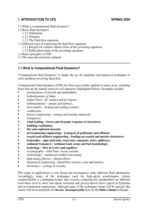
Computational Fluid Dynamics – or How to Make a Good Boat FastDavid VacantiThe term CFD is showing up more often these days in articles describing the design efforts used to make Volvo 60 round the world racers and America’s Cup yachts faster. Computational Fluid Dynamics or CFD actually covers a great many engineering specialties and is not the sole domain of boat and ship design. In this article we will review what types of CFD products exist and hopefully provide some understanding of when and how CFD products are best suited to a project. Computational Fluid Dynamics is the application of computers to the modeling of fluid characteristics when either the fluid is in motion or when an object disturbs a fluid. A few examples of a fluid in motion are water or chemical flow in pipes, heating and ventilation systems conducting cooling, heating or fresh air supplies to a building. Fluids in motion also include flame and fire effects in combustion or jet engines. Surprised by these fields of interest?What about examples of an object disturbing a fluid? Examples include stirring paddles submerged in a tank of water and effluent in a waste treatment plant, aircraft of all kinds, cars and trucks at highway or racing speeds and even monohull sailboats, ship, multihull sailboats to name but a few. Obviously, an open mind is important when considering what constitutes a fluid. Fluids can exist in gaseous and liquid states and science has recently found that even some solids can exhibit fluid like characteristics under right conditions. Scientists have found that some of the most spectacular and deadly landslides or rock falls behave as a fluid while the mass of stone and soil or sand is in motion, only to return to a most decidedly solid form when the motion subsides.The general field of fluid dynamics differs from the field of boat design in one critical way. Onlyboat design deals with a vehicle passing through the two fluids of air and water simultaneously.Our atmosphere is a compressible fluid, though not at yachting or even high-powered boat racing speeds. Air can change in density according to altitude, temperature and humidity. Water is an incompressible fluid that can vary in viscosity according to its salinity and temperature.For most of us, small effects such as variable salinity and temperature are not of concern, but can make the difference between winning and loosing a major international yacht race.How do CFD programs Work?CFD programs are based on the laws of physics, such as the law of conservation of momentum, and special “boundary conditions”. The law of conservation of momentum states that the total momentum of a system remains constant regardless of how the system may change. A boundary condition limits how and where a fluid can travel. A simple example is that motion of the fluid must remain tangent or parallel to the surface of an object passing through it. Another example is that pressure applied by the fluid against the object must be perpendicular to the surface at all points. These laws and conditions are critical to the development of a CFD program because they allow an aerodynamicist to write equations that describe the system that is being studied. Without the physical laws and boundary conditions there would be no way to write equations that describe fluid motion. The complex equations that result take into account the viscosity, mass and other characteristics of the fluid. The equations are written using integral and differential calculus and require specialized computer techniques to solve them. Typically the programmer writes an algorithm that makes a series of estimates using algorithms that iteratively solve the sets of equations by looking for “balance” in the system of equations. A final answer is obtained when the algorithm converges on a solution with an error that is sufficiently small for the desired accuracy. Once an algorithm has been developed to implement the laws of momentum and boundary conditions, it cannot be applied to the entire surface of the hull and appendages at once. The surface area of the hull, keel and rudder are broken into thousands of small patches (collectively called a mesh) and the algorithm applied to each patch. Each patch in turn influences the fluid flow on the patch area of its neighbors and therefore the solution must account for the conditions surrounding the patch currently being solved. As a result the program must solve and resolve the equations for all of the patches until the solution obeys the physical laws and boundary conditions. Sometimes the complexities of the laws of physics are too difficult to implement all at the same time. As a result the aerodynamicists choose to write programs that make certain limiting assumptions that permit the programming to become more practical and still result in reasonable results. A specific example arises in the case of what actually happens to fluids very near the surface of an object. The boundary layer as it is called experiences shear forces in the objects direction of travel that result in viscous drag. These shear forces are described in a special set of equations called the Navier Stokes relationships. The Navier Stokes equations are sufficiently complex themselves that attempting to include them within every aerodynamics or hydrodynamics program would make the solutions nearly impossible. As a result there are Navier Stokes based programs that specifically address viscous drag and Panel method programs that compute lift, wave drag and induced drag. A complete estimate of the drag encountered by a boat requires the data supplied by both programs.What do CFD programs Calculate?The most obvious calculation that would be of interest in boat design is the determination of drag forces. But drag comes in several forms that can include, wave, viscous, and induced drag. Therefore, a designer must evaluate the effects of his design in each of these drag areas. The second general area of calculation is lift. The term lift arises from its application to aircraft and becomes a bit confusing when applied to the field of boat design. Lift applies to the forces generated by a keel or centerboard to resist the side force of sails and the driving force of the sails themselves. It also applies to the turning forces of a rudder, and the supportive force acting on “foils” to elevate a hydrofoil sail or powerboat above the water surface.There is also a distinction between 2 and 3 dimensional fluid dynamics analysis. Specifically, there are programs that predict the performance of foils as if they existed on a wing of infinite length. Here the term “foil” is used to define the shape of a keel or rudder along the chord from the leading to the trailing edge. Foil shapes are best known by the alphanumerical names given to them such as NACA 63A012. So a 2D fluids program would compute the lift, drag, velocity distribution, turbulence onset and the generation of bubbles similar to cavitation for a 2D shape such as a wing or keel foil, and would not include any 3D information such as keel span or thickness distribution or the presence of a bulb. A 3D fluids program would compute wave and induced drag from a hull, keel and rudder, including the effects of a bulbed keel carrying winglets.CFD codes are critical for more than optimizing the performance of a top-notch America’s Cup class racing yacht. These codes can be of great value to determine loads placed on boat structures of all types and are invaluable when applied to unique marine structures such as oil platforms that are frequently subjected to the world’s worst storms.Lift and drag effects translate directly into loads that must be sustained by the boat or oil derrick if it is to remain intact in its intended operational conditions. For example, several years ago when the race was known as the Whitbread Round The World Race, many boats developed life threatening hull delamination when subjected to the continuous pounding of high speed downwind surfing and upwind beating. While delamination of a boat at sea is definitely related to structural design errors, those errors were caused by a lack of detailed information about the fluid forces experienced by the boats. Knowledge of these forces would have enabled designers to prevent the hull damage in the first place.Therefore, the potential application of CFD to your design project should depend on whether or not the design regime that your vessel will operate in has well understood engineering data available to prevent hull damage in addition to overall performance of the vessel. For example, the last few years have seen the development of high-speed hydrofoil sailboats for the consumer market. These top performance boats experience not only significant speeds and loads, but the potential for unstable characteristics could make it highly dangerous to ride in one. However, the judicious use of field-testing and computer analysis has produced a crop of very exciting hydrofoil sport boats that are a joy to fly in.Finally, several years ago a multihull sailboat arrived in port after participating in a trans-Atlantic race. When the centerboards were raised in the outer hulls of the trimaran, the skipper wasshocked to learn that the boards had been sheered off just below hull depth and he had not had their use for some indeterminate time during the later portion of the race. Clearly, the structural design of the boards had not taken into account the true forces of lift, drag or perhaps cavitation that would be experienced at sea.CFD programs do not calculate how fast a boat of any type will pass through the water or predict the time to complete a course around the buoys. Predicting speed on a racecourse is the domain of another class of programs called Velocity Prediction Programs or VPP. The VPP makes use of lift and drag numbers calculated in a CFD program to estimate the speed about will sail a course given the sail drive forces and the stability or righting moment of the hull. The VPP is a closed loop simulation continuously varies estimated speed and resulting lift, drag and righting forces until retarding and driving forces are balanced and a stable speed results. A CFD program on the other hand is an open loop simulation that simply states that given an angle of heel and speed for a specified hull and appendage configuration, here are the forces that will result for that instant in time. No consideration is given to how the vessel achieved that speed or sailing condition.In summary then, CFD programs not only calculate lift and drag forces of a hull with appendages, they can also be used to compute pressure loads due to waves and wave impact at speed. The forces of lift, drag and pressure can be translated into structural requirements and provide the means to optimize a hull working in concert with its appendages to produce lift in the most efficient manner possible while satisfying the needs for stability. Predictions of lift and drag at various speeds can be used to develop a mathematical model needed to accurately close the analysis loop of a velocity prediction program.When is a CFD Computer Program Required?CFD codes are not always required or justified however, when simpler means of estimating the forces involved are available. In the case of a typical sailboat design, the forces generated by the keel and rudder can be easily estimated if the keel lacks a bulb and if the keel and rudder shape are essentially straight leading and trailing edges. It is possible to make use of analytical methods that are easily implemented on personal computers. A simple example is the program I wrote called LOFT that makes use of analytical methods developed by NASA and the US Air Force for initial performance prediction of wing designs.However, while simple programs like LOFT can adequately address typical bulb-less keels and rudders they cannot analyze the performance of an America’s Cup racing keel with bulb and winglets. Only 3D CFD programs can address that complex task.Who can operate a CFD program?While CFD programs can be of tremendous value, getting accurate and meaningful results is not typically within the reach of amateur and many professional boat designers. A degreed Naval Architect or a fluids dynamicist is required to generate the key initial input to a CFD program called a mesh.The mesh is a mathematical description of the hull and appendages that are to be analyzed. It is not sufficient or even possible to use standard stations, waterlines and buttocks as inputs to a CFD program. The detailed shapes of the hull and appendages must be defined by a mesh of squarepatches that adjoin one another and whose dimensions are chosen according to the local curvature of the hull or appendage or by the occurrence of the intersection of the hull and a keel, rudder or lifting strut of a hydrofoil. The generation of a mesh is a science unto itself and can require iterations by the analysts running successive trials to be sure that the mesh is sufficiently dense in critical areas. Some meshing can be done automatically and then refined by hand.Typically the developers run complex 3D CFD programs or thosetrained in their use and as result are not really meant for use by therest of us. However, 2D fluids programs designed for the analysisand development of 2D air or hydrofoil shapes (recall the 63A010example) are sufficiently easy to use for a designer with basicmathematics skills and general knowledge of airfoil characteristics.Analytical programs such as Vacanti Yacht Design’s FOIL programcan aero / hydrofoil lift, drag, turbulence onset and bubbleformation characteristics for anyone with basic computer skills anda working knowledge of basic foil design.What CFD Programs Exist?Panel Method and Navier Stokes programs are two generalclasses of CFD programs that apply to the issues of boat design.The most commonly used and most available are Panel Method programs. Panel methods allow the prediction of wave drag, free surface effects and induced drag due to lift generated by a keel or rudder but they do not account for viscous drag. Programs using panel methods assume that there are only forces normal to the surface of the hull within the fluid. However, due to viscosity, the fluid is subject to forces in shear – more or less parallel to the hull surface that causes turbulence. Therefore the panel programs are referred to as “inviscid” analysis methods. As a result they compute wave and induced drag but not the effects of viscous drag. Viscous drag computations are computed by specialized codes known as Navier Stokes programs. These programs are difficult to use and apply and are best left to a professional skilled in their use. When a designer has a task that justifies the use of CFD programs, he should be using design tools that that can export true 3D surface shapes in the form of common Computer Aided Design (CAD) file formats. Designing in a typical CAD program such as AutoCAD using lines and polylines, even though in 3D are not sufficient for use with CFD programs. True surface definitions such as Non-Uniform Rational B-spline (NURB) surfaces are required. Most professional versions of the commonly known yacht design programs (AeroHydro, AutoShip, Maxsurf, New Wave, PROLINES) all provide this kind of file exchange.Licensing costs or consulting time is available from the companies or sources listed below.Company Name Program(s) Web AddressAerologic Cmarc,Postmarc/dwt.htmlAnalytical Methods Inc VSAERO,FSWAVEFluent FLUENT/solutions/marine/index.htm South BaySimulationsSPLASH /~brosenVacanti YachtDesignFOIL 97 Virginia Technical University Several Freesimple programs– Code Compilermay be required/aoe/faculty/marchman/softwareCFD Online Very extensivelinks to manysuppliers of CFDprograms ofevery possibletypeSpecialized consulting companies include:Bruce RosenSouth Bay Simulations44 Sumpwams AveBabylon, NY 11702 631 587 3770, brosen@Joe LaisoaFluid Motion Analysis Consulting, Inc.3062 Queensberry Dr.Huntingtown, MD 20639, 410 535 0307 X3351, laiosa@ConclusionCFD programs are best applied when there are either significant engineering unknown effects or load levels or where design optimization for a specific application in specific conditions are essential to the goal. For instance, there are many books of scantlings or building standards for typical sailboat or powerboat designs intended for inland cruising. But an attempt at the world record speed sailing at the “ditch” in France at speeds approaching 50 knots clearly calls for specialized analysis to prevent catastrophic failure that could risk lives or incur that last bit of drag that could prevent success in inching the speed record that much higher.Some CFD codes are only usable in the hands of a skilled practioner and others are designed and intended for use by those with reasonable technical skills and willingness to do a bit of reading or research to help them understand the results and limitations of their modeling efforts. CFD andanalytical programs are very important to the development of high performance vessels from the perspective of optimization for speed and safety. High speed sailing craft and those destined for offshore use can benefit the most from computer analysis methods. One final key point here is that we have only discussed vessels in displacement mode and have not referred to high performance planning powerboats. The prediction of planning vessel performance is an art unto itself and is the domain of yet another class of programs. I refer those of you who wish to know more about that subject area to research the Society of Naval Architects and Marine Engineers() web site.。

NX Flow uses computational fluid dynamics (CFD)to accurately and efficiently simulate fluid flow and convection.An element-based,finite volume CFD scheme is used to compute 3D fluid velocity,temperature and pressure by solving the Navier-Stokes equations.The NX Flow technology allows a user to model complex fluid flow problems.The solver and modeling features include:•Steady-state and transient analysis (adaptive correction multigrid solver)•Unstructured fluid meshes (supports tetrahedral,brick and wedge element types)•Skin mesh (boundary layer mesh)•Complete set of automatic and/or manual meshing options for the selected fluid domains•T urbulent (k-ε,mixing length),laminar and mixed flows•CFD solution intermediate results recovery and restart•Heat loads and temperature restraints on the fluid•Forced,natural and mixed convection•Fluid buoyancy•Multiple enclosures•Multiple fluids•Internal or external flows•Complete and seamless coupling to NX Thermal for simulation of conjugate heat transfer (handlesdisjoint meshes at fluid/solid boundaries)•Losses in fluid flow due to screens,filters and other fluid obstructions (including orthotropicporous blockages)•Head loss inlets and openings (fixed or proportional to calculated velocity or squared velocity)•Fluid swirl at inlet and internal fans NX FlowComputational fluid dynamics (CFD)to accurately and efficiently simulate fluid flowand convectionNX/plmfact sheetBenefitsAllows for investigation of multiple ‘what-if’scenarios involving complex assembliesAllows the selection of a bounding volume around complex geometry to specify external boundaries of the fluid domainProvides extensive set of tools for creating CFD analysis-ready geometryBy default,all 2D and 3D solids will transfer heat to the fluid they adjoin and serve as obstruction to the fluid ers can control the surface roughness and walls convective properties globally and locally Features Automatic connection between disjoint fluid meshes within an assembly Option for automatic fluid mesh created at run time NX integrated CFD solution toolset Geometry modeling and abstraction toolset All solid surfaces obstructing the fluid can automatically transfer heat to the fluid they adjoin Handling of disjoint meshes at the fluid/solid boundaries for conjugate heat transferSummaryNX ®Flow software is a computational fluid dynamics (CFD)solution that is fully integrated into the native NX Advanced Simulation environment.It provides sophisticated tools to simulate fluid flow and heat transfer for complex parts and assemblies.The integrated CFD solution allows fast and accurate fluid flow simulations and provides insight into product performance during all design development phases,limiting costly,time consuming prototype testing cycles.NX Flow simulation requirements and applications are typical to these industries:aerospace and defense,automotive,consumer products,high-tech electronics,medical,power generation and process.Siemens PLM Softwaresolid surfaces will automaticallyadjoin.Similarly,all volumes thatnot already defined as flowfrom their surfaces as well.suite of Advanced Simulation applications available within theeither NX Advanced FEM or NX Advanced Simulation as awith NX Thermal,NX Flow provides a coupled multi-physicsapplications.hardware platforms and operating systems including Unix,Windows ContactSiemens PLM SoftwareAmericas8004985351Europe44(0)1276702000Asia-Pacific852********/plm©2007Siemens Product Lifecycle Management Software Inc.All rights reserved.Siemens and the Siemens logo are registered trademarks of Siemens AG.T eamcenter,NX,Solid Edge,T ecnomatix,Parasolid,Femap,I-deas,JT,UGS Velocity Series and Geolus are trademarks or registered trademarks of Siemens Product Lifecycle Management Software Inc.or its subsidiaries in the United States and in other countries.All other logos,trademarks,registered trademarks or service marks used herein are the property of their respective holders.10/07。

CFD的含义Computational Fluid Dynamics, 即计算流体动力学。

CFD软件(Computational Fluid Dynamics, 即计算流体动力学, 简称CFD [ 1 ] ) 是目前国际上一个强有力的研究领域, 是进行传热、传质、动量传递及燃烧、多相流和化学反应研究的核心和重要技术, 广泛应用于航天设计、汽车设计、生物医学工业、化工处理工业、涡轮机设计、半导体设计、HAVC&R 等诸多工程领域, 板翅式换热器设计是CFD 技术应用的重要领域之一。

CFD 在最近20 年中得到飞速的发展, 除了计算机硬件工业的发展给它提供了坚实的物质基础外, 还主要因为无论分析的方法或实验的方法都有较大的限制, 例如由于问题的复杂性, 既无法作分析解, 也因费用昂贵而无力进行实验确定, 而CFD 的方法正具有成本低和能模拟较复杂或较理想的过程等优点。

经过一定考核的CFD 软件可以拓宽实验研究的范围, 减少成本昂贵的实验工作量。

在给定的参数下用计算机对现象进行一次数值模拟相当于进行一次数值实验, 历史上也曾有过首先由CFD 数值模拟发现新现象而后由实验予以证实的例子。

CFD 软件一般都能推出多种优化的物理模型[ 2 ] , 如定常和非定常流动、层流、紊流、不可压缩和可压缩流动、传热、化学反应等等。

对每一种物理问题的流动特点, 都有适合它的数值解法, 用户可对显式或隐式差分格式进行选择, 以期在计算速度、稳定性和精度等方面达到最佳。

CFD 软件之间可以方便地进行数值交换, 并采用统一的前、后处理工具, 这就省却了科研工作者在计算机方法、编程、前后处理等方面投入的重复、低效的劳动, 而可以将主要精力和智慧用于物理问题本身的探索上。

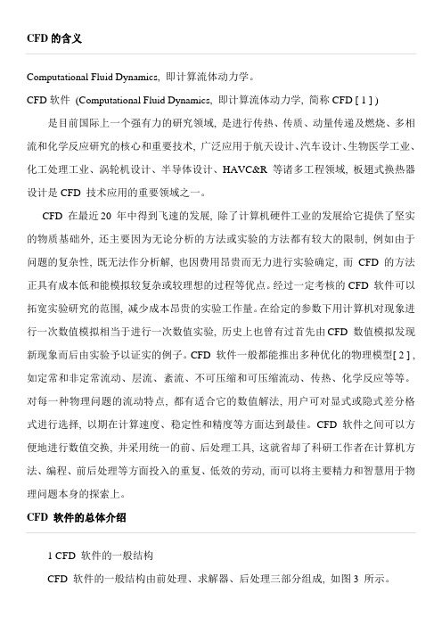
CFD 软件的总体介绍1 CFD 软件的一般结构CFD 软件的一般结构由前处理、求解器、后处理三部分组成, 如图3 所示。

前处理、求解器及后处理三大模块, 各有其独特的作用, 分别表示如下:一般结构前处理a. 几何模型b. 划分网格求解器a. 确定CFD 方法的控制方程b. 选择离散方法进行离散c. 选用数值计算方法d. 输入相关参数后处理速度场、温度场、压力场及其它参数的计算机可视化及动画处理商业软件介绍自从1981 年英国CHAM 公司首先推出求解流动与传热问题的商业软件PHO EN ICS以来, 迅速在国际软件产业中形成了通称为CFD 软件的产业市场。

CADFEM eNewsletterA tri-annual newsletter from CADFEM India September 2010 Volume 3, Issue 1Massive Parallel Programming in LS-DYNAIllustration: Speed up using SMP and MPPNonlinearities of Anisotropic MaterialsIllustration: 3-point bending – Force vs. deformationHybrid Simulations for Hybrid VehiclesC ONTENTSNonlinearities of 2Anisotropic MaterialsHybrid Simulations for 4 Hybrid VehiclesElectro-thermal 6 simulations for batteries Robustness Study – 7 Automotive ApplicationMassive Parallel Prog. 8in LS-DYNA CAE News & Events 11About Us 12We welcome you to a brand new edition of the CADFEM eNewsletter that shall update you some of our articles along withthe latest news & events from the CAE industry. High performance computing is the order of today. It only makes sense to utilize the available computational power for running our simulation tasks. One of the key articles in this edition of the newsletter talks just about massive parallel processing (MPP) specifically for LS-DYNA users. Several other articles in eclectic analysis areas are also discussed. Hope you enjoy reading this edition too and find it informative. Please feel free to send us your suggestions for improvement. If you wish to contribute to the newsletter as a guest author, then please feel free to contact us.S UBSCRIBEVisit our Subscription Center E VENTS2010 ANSYS India ConferenceOctober26 – 27, 2010 Bangalore, India October29, 2010 Pune, IndiaANSYS Conference & 28th CADFEM Users’ Meeting November 3 – November 5, 2010Aachen, GermanyIt is a well known fact in the automotive industry that the future breed of vehicles will largely carry electric traction and hybrid-electric propulsion. With the improved technology there is no wonder that the high level of intricacy and wide variety of domains involved in this kind of design has appropriate simulation and analysis tools.… (details on page 4)Theanisotropic,nonlinear,strain-ratedependency, the interface between polymer matrix and fiber, fiber length, fiber orientation in the composite makes the composite material complex enough for the engineering study. Howone can model the material and ensure accurate structural modeling is discussed here.… (continued on page 2)There are two versions of LS-DYNA, Shared MemoryParallelization (SMP) and Massive Parallel Processing(MPP). The MPP version of LS-DYNA has been developed by LSTC throughout the 1990‟s. A primary goal for the code has been superior scalability, enabling many processors to work together efficiently in the execution of LS-DYNA.… (continued on page 8)2 CADFEM eNewsletterSeptember 2010 Volume 3, Issue 1Nonlinearities of Anisotropic MaterialsMulti-Scale Material & Structural Modeling using DIGIMATThe accurate linear and nonlinear modeling of complex composite structures pushes the limitsof finite element analysis with respect to element formulation, solver performance and phenomenological material models. The finite element analysis of injection molded structures made of nonlinear and/or time-dependent anisotropic reinforced polymer is increasingly complex. In this case, the material behavior can significantly vary from one part to another throughout the structure and even from oneintegration point to the next in the plane and across the thickness of the structure due to the fiber orientation induced by the polymer flow. The accurate modeling of such structures and materials is possible with LS-DYNA using LS-DYNA‟s Usermat subroutine to call the DIGIMAT micromechanical modeling software.(1)(2) In addition to enabling accurate and predictive modeling of such materials and structures, thismulti-scale approach provides the FEA analyst and part designer with an explicit link between the parameters describing the microstructure (e.g. fiber-orientation predicted by injection molding software and the final part performance.Material DescriptionAs material, which is investigated in this work, a PA66+PA6I/6T LGF50 is chosen. The material is supplied by the EMS-CHEMIE AG, where the material with the name GRIVORY GVL-5H can be characterized as a high performance long glass fiber reinforced thermoplastic for applications with medium temperature, high strength and stiffness requirements combined with excellent processing and low warpage behavior.Long fiber reinforced thermoplastics (LFRT) have in comparison to short fiber reinforced thermoplastics(SFRT)longerfibers.Forexample, the fiber length of a SFRT granulate is between 0.2 and 0.8 mm. On the other hand the fiber length of a LFRT granulates is app. 10 mm (see Fig. 1). Theanisotropic,nonlinear,strain-ratedependency, the interface between polymer matrix and fiber, fiber length, fiber orientation in the composite makes the composite material complex enough for the engineering study. In the traditional simulations (see Fig. 2), the material models will not consider the local material parameter in the simulation. This results in the study of the composite material at the macro level. In the multi-scale material modeling simulation (Integrative Simulation) the local material parameter will be considered. This helps to understand the behavior of polymer matrix, fiber material separately (micro scale) and also analyze the composite material (macro scale).Multi-Scale Material Modeling Platform The software solution, DIGIMAT, offers the user a complete set of tools that allows the coupling between injection molding simulation and structural analysis for the fiber-reinforced plastic parts. DIGIMAT takes the locally different microscopic glass fiber orientations of the part into consideration. These differences are caused by the viscous flow of molten plastic during processing of the part leading to a variation of the microstructure over the plastic part which getssolidifiedaftercoolingtoroomtemperature. The material is anisotropic because of the locally oriented fibers. In principle, for each element in the structural analysis an individual material description has to be used (see Fig. 3).(continued in the next page)AuthorChandra Sekhar KattamuriInterested in more details?Email us atconsulting@cadfem.in for further information.Fig 1: Comparison between 3 mm SFRT(left) and 11 mm LFRT granulate (right) Image courtesy: EMS Grivory AGFig 2: Traditional Simulation vs.Integrative SimulationFig 3: Multi-scale Material ModelingPlatform - DIGIMATCADFEM eNewsletter 3 September 2010 Volume 3 Issue 1Nonlinearities of Anisotropic MaterialsMulti-Scale Material & Structural Modeling using DIGIMATWorkflow of a coupled DIGIMAT analysis The standard workflow of an integrated DIGIMAT analysis commonly starts with the reverse engineering of material properties within DIGIMAT-MF. In DIGIMAT-MF, the constitutional behavior of the matrix and the filler phase is defined separately through a set of parameters for predefined mathematical functions. These parameters are derived from the experimental stress strain curves for the respective material. Often only measurements for the complete composite material are at hand. In these cases the average microstructure of the test specimen is taken as a set value and the composite material parameters can be reverse engineered by the use of DIGIMAT-MF.Once the parameters are known they are kept fixed and the influence of the microstructure on the material behavior can be investigated. It is this sensitivity towards a change in the microscopic fiber orientation which is taken into account by setting up a coupled analysis with results from injection molding simulations. MAP is a 3D mapping software used to transfer the fiber orientation, residual stresses and temperatures from the injection molding mesh to the structural analysis mesh.Once the material parameters and fiber orientation files are ready, this information has to be linked with the structural simulation. DIGIMAT to CAE is the multi-scale structural modeling tool that groups the interfaces between injection molding software, DIGIMAT-MF and structural analysis software.SimulationsGeneral purpose finite element software LS-DYNA is used for running traditional simulations. *MAT_MODIFIED_PIECEWISE_LINEAR_PLASTICI considered. This material model has beenselected upon validating the test results withvarious material models available in LS-DYNA. Inthe automotive industry this is one of the mostpopularly used material models for FRP materials.Three different tests have been considered –Uniaxial Tensile test, Three-Point Bending Testand Impact Test.∙Uniaxial Tensile test shows that bothtraditional simulation using LS-DYNA andintegrative simulation using DIGIMAT to LS-DYNA interface produce good results. Thesimulation results fit very well with theexperiment (see Fig. 4).∙The result of the Three-Point Bending testclearly shows that the traditional simulation isnot able to capture the material behaviortransversal to the fiber direction. This isbecause *MAT_123 is basically an isotropicmaterial model and anisotropic materialbehavior cannot be captured. Results of theintegrative simulation, on the other hand, fitswell with the experiment (see Fig. 5).∙Traditional Simulation result of the Impact testtells us the material fails much earlier thanwhat is seen in the experiment. Withintegrative simulation, the material behavior iscaptured properly (see Fig. 6).ConclusionsThe material considered, GRIVORY GVL-5H, along glass fiber reinforced thermoplastic is seento be an anisotropic, nonlinear, strain-ratesensitive material. Traditional results do not givecomplete confidence which can otherwise begained through integrative simulation. DIGIMATis seen to be a proven tool for capturing materialbehavior in an accurate manner.Fig 4: Uniaxial Tensile Test Results –Comparison between Traditional andIntegrative SimulationFig 5: Three Point Bending TestResults – Comparison betweenTraditional and Integrative SimulationFig 6: Impact Test – Comparisonbetween Traditional and IntegrativesimulationReferences1.http://www.cadfem.in/products/digimat.html2./3.L. Adam, A. Depouhon & R.Assaker: Multi Scale Modeling ofCrash & Failure of ReinforcedPlastics Parts with DIGIMAT to LS-DYNA interface 7th European LS-DYNA Conference, 2009.4.Dr. Jan Seyfarth, Dr.-Ing. MatthiasHörmann, Dr.-Ing. Roger AssakerChandra S. Kattamuri, BastianGrass: Taking into Account GlassFiber Reinforcement in PolymerMaterials: the Non LinearDescription of AnisotropicComposites via the DIGIMAT to LS-DYNA Interface, 7th European LS-DYNA Conference, 2009.4 CADFEM eNewsletterSeptember 2010 Volume 3, Issue 1Hybrid Simulations for Hybrid VehiclesImportance of co-simulation for modeling vehicle propulsionGrowing importance of Hybrid vehicles It is a well known fact in the automotive industry that the future breed of vehicles will largely carry electric traction and hybrid-electric propulsion. These kind of propulsion are inherently more complicated than conventional vehicles which are built exclusively with internalcombustion engines.Importance of simulationsDifferent technologies grow at different parts of the world, forming a decentralized design process. The complete assembly of a vehicle consists of several subsystems that must work together in the vehicle. Each of these subsystems are manufactured at different continents and finally assembled into a single vehicle. In this trend, it is logistically complex and tedious to bring the testing equipment together to validate the behavior of complete assembly. The only feasible method to explore design variations is numerical simulations . With the improved technology there is no wonder that the high level of intricacy and wide variety of domains involved in this kind of design hasappropriate simulation and analysis tools.The hybrid vehicle propulsionIn particular, there has been much attention paid to the modeling of automotive drivetrains or powertrains. In hybrid vehicles, there is a dominating number of electrical systems. For example, a typical hybrid drivetrain consists of all the components that generate power, convert power and deliver it to the wheels. This includes the engine, transmission, energy storage device, motors and motor controller, driveshafts, differentials, and the wheels.Simulations at different levelsNumerical modeling and simulation of these subsystems can be carried out at different levelsof details. For example, there are simulations for calculation of efficiency maps of electric machines (fig. 2). In an another way of modeling the motor which is at a system level the motor is just a black box that generates specific outputs in response to inputs.Simulating complete drivetrainsMany other vehicular subsystems such as electronic inverters, regenerative brakes, and various kinds of actuators can be modeled the same way. System level models can now predict how the overall system will behave. The system level simulation gets inputs and works with detailed electrical models of component parts (fig. 1). Use of these simulation packages lets automotive engineers work in a single integrated design environment. Software can help predict efficiency and fuel economy of vehicle designs, power management strategies, and guide the electricaldesign.Engineerscansimulatecomplete drivetrains by combining fuel cells, batteries, power electronics, and electric motors in one environment. Most of such components are modeled and available for use as multiple designs.Complex vehicle detailsThe electrical components for vehicles can be extremely sophisticated due to the increased technology. They are manufactured with a lot of design features to minimize costs and optimize efficiency. Similarly, it is important for drivetrain simulations to accurately model these features to the level of electric field properties, torque qualities, and other details. These details provide a foundation for system level simulations allowing accurate simulation for the behavior of complete assembly.(continued in the next page)Fig 4: Different levels of modelingFig 5: Calculation of efficiency maps ofelectric machines (component model with real time capabilty)Fig 6: Motor design in RM-Expert (component model with high computational effort)Interested?For details, you may contact us at info@cadfem.inAuthorSreekanth NallaboluCADFEM eNewsletter 5 September 2010 Volume 3 Issue 1Hybrid Simulations for Hybrid VehiclesImportance of co-simulation for modeling vehicle propulsionCapabilities for co-simulationDue to the lack of a distinct comprehensive environment for combining all the models, one can synergize several simulation tools to give designers feel of how motors, drives, and other electromechanical systems will interact. The software, RMxprt is a specialized software for the design of rotating electric machines (fig.2) which has the capability to calculate key performance metrics of electric motors. One can evaluate design tradeoffs early in the design process. It computes performance of specific designs through a combination of classical analytical motor theory and equivalent magnetic circuit methods. RMxprt also can create statespace system models incorporating the physical dimensions of the machine being designed, winding topologies and nonlinear material properties. These factors can then be transferred to another simulation package called Maxwell 3D.Maxwell3D uses finite-element methods to solve electromagnetic-field problems in the time and frequency domains. It is typically used to analyze the fields (fig.3) associated with electromagnetic actuators and components. Using Maxwell 3D, one can solve for electromagnetic-field quantities such as force, torque, capacitance, inductance, resistance, and impedance. One can also generate state-space models using this tool to help optimize design performance.Engineers can use the Rmxprt state-space model to explore electronic control topologies, loads, and interactions with drive-system components in another simulation package called Simplorer (fig 5). Simplorer is a simulator specifically for system simulation including power electronics.In Simplorer one can model at a system levelusing several standard languages like VHDL-AMS,SPICE, SML,C/C++ etc. VHDL-AMS is alanguage standard for the description andsimulation of multidisciplinary mixed-signalsystems. RMxprt design and Maxwell can work ina Simplorer environment to define the behaviorof rotational actuators in the hybrid drivetrain.Models developed this way can be configured indifferent design domains at different levels ofabstraction. This sort of description also lets themodel be co-simulated with specializedsimulation packages and proprietary code,linking to Maxwell for high-fidelity modeling ofelectromechanical components.Within Simplorer one can model componentsusing several modeling techniques like Blockdiagrams, State machines or Circuits. One canalso perform optimization at system level. Inaddition one can co-simulate with third partytools like Matlab Simulink, MathCAD etc.Simplorer has a unique capability to combinedifferent modeling techniques in a singleenvironment. A very nice example is theintegration of a Lithium-ion cell with thecomplete battery. One would like to model thecomplete battery pack using block diagrams inorder to combine it with the other vehiclesubsystems. But modeling the detailedelectrochemistry at cell level is done usingequivalent circuits or programming the physicsusing VHDL-AMS. Once can then make thisphysics based cell model with the block diagrambased battery model with in Simplorerseamlessly. All these examples gives a brief ideaof the multidomain and multilevel capabilitiespossible with co-simulation, though there ismuch more to explore.Fig 4: Electro-magnetic analysis of electricmachine design (component model with highcomputational effort)Fig 5:Co-simulation in SimplorerImages courtesyFig. 3, 4 & 5 – Ansoft Inc.AuthorSreekanth NallaboluInterested?For details, you may contactus at info@cadfem.in6 CADFEM eNewsletterSeptember 2010 Volume 3, Issue 1Electro-thermal simulations for batteriesA reviewIntroductionElectrochemical batteries are of significant importance in electrical power systems since they give a means for energy storage in a way that is immediately available and pollution free.Few key applications that have grew fast during last decade are: Batteries within Uninterrupted Power Supplies (UPS), Battery Energy Storage Plants (BESP) to be installed in power grids, electric vehicles. There are several battery technologies that are currently being used, the more widespread being the lead-acid and Li-ion technologies.Simulation driven development of Battery One would like to simulate a battery at two different levels. The first being detailed cell level simulation involving the electrochemistry and the other being system level simulation of the entire battery consisting of several cells. On battery cell level, the focus is on detailed heat generationand temperature distribution within a battery cell. This type of study is pursued mainly by battery manufacturers and battery researchers. Experimental data reveals that the rate of heat generation varied substantially with time over the course of charging and discharging. Heat can be generated from internal losses of Joule heating and local electrode overpotentials, the entropy of the cell reaction, heat of mixing, and side reactions. Considering only Joule heating andlocalelectrodeoverpotentials,heatgeneration can be expressed by open circuit potential and potential difference between the positive and negative electrodes.One can model the cell either as a detailed physics based model or as an equivalent circuit. Physics based electrochemistry model, can be used to investigate the impact of battery design parameters on battery performance, which includes the geometry parameters, properties,and temperature. Equivalent circuits are a workaround for detailed time consuming physical modeling.Challenges in Battery designThe lithium-ion battery is ideally suitable as a power source for hybrid electric vehicle (HEV) and electric vehicle (EV) due to its uniqueness such as high energy density, high voltage, low self-discharge rate, and good stability among others. There are several causes of failure of a battery. Heat is a major battery killer, either excess of it or lack of it, and Lithium secondary cells need careful temperature control to avoid thermal runaway. Due to likelihood of significant temperature increase in large batteries during high power extraction safety is currently one of the major concerns confronting development of lithium batteries for electric vehicles. A properly designed thermal management system will be crucial to prevent overheating and uneven heating across a large battery pack, which can lead to degradation or mismatch in cell capacity. Design of the thermal management system requires knowledge about the cooling system as well as the amount of heat that will be generated by cells within the battery pack.The so called battery aging is also one of the interesting aspects for battery specialists. Battery life and reliability forms a key feature of interest in the automotive industry. For product designers, an understanding of the factors affecting battery life is vitally important for managing both product performance and warranty liabilities particularly with high cost, high power batteries. Offer too low a warranty period and you won't sell any batteries/products. Overestimate the battery lifetime and you could lose a fortune. In spite of being so important decision maker modeling of battery aging is still ambiguous is the market.Fig 7: Electrochemistry in Lithium-ion cellFig 8: Electrothermal simulation of batteryInterested?For details, you may contact us at consulting@cadfem.inAuthorSreekanth NallaboluCADFEM eNewsletter 7 September 2010 Volume 3 Issue 1Robustness Study – Automotive applicationStochastic studies to determine robustness of NVH of a Brake SystemThe automotive industry is one of the drivers of CAE-based virtual product development. Due to a highly competitive market, development of innovative, high quality products within a short time is necessary and it is only possible by using virtual prototyping. It is important to note that increased application of virtual prototyping itself increases the necessity to perform robustness studies.Brake noise is one of the most important problems in the automobile industry due to the high warranty costs. The generation of brake noise is due to the development of instabilities in the brake system. The analysis of brake squeal is highly complex, which is very sensitive to the operation conditions. Robustness analysis is primarily carried out to determine the variation range of significant response variables and their evaluation by using definitions of system robustness due to the imperfections of design parameters. The imperfections are usually modelled by either random variables that are constant in space or random fields that vary in space.Occurrence of squeal is intermittent or perhaps even random. Many different factors appear to affect squeal. Out of which, one of the factor is existence of tolerances in material of the brake system (see Fig. 1) in reality. Therefore, robustness analysis has been carried out by considering the material tolerances for thorough understanding of brake squeal. Robustness analysis is carried out by stochastic modelling of material tolerances by random variables by software called optiSLang.Keywords:Stochastic Finite Elements, Robustness Analysis, Brake Squeal. Robustness Analysis Using MaterialTolerancesDesign parameters are the Young‟s modulus ofeach component. Components and theretolerances of Young‟s modulus are given in Table1. The coefficient of variation and distributions ofYoung‟s Modules of different components isselected based on engineering experiences. Thetruncated normal function is chosen as the PDFfor all parameters with the bounds equal to twotimes coefficient of variation.Robustness analysis is carried out for 100 designsin this case, to get a clear idea about thevariation of response parameter w.r.t thevariation of design parameters. From Fig. 2 it isobserved that the variation of design parametersleads to a high variation is the responseparameter which is the squeal propensity.From analysis Pad G33, which means stiffness ofpad in out of plane direction is the mostinfluential design parameter and it has linearcorrelation with the response. The mean ofdamping ratio (from Fig. 3) for all designs is0.048 which is high in terms of squeal noise. It isalso observed that the coefficient of variation(CV) is about 45% which in turn indicates thatthe brake system is not robust.SummaryIn the virtual model, the phenomenon which isfound in the tests could be retrieved byrobustness analysis. Primary result of therobustness evaluation is the estimation of thescatter of important result variables. Furthermoresensitive scattering input variables can beidentified as well as the determination of resultvariables can be examined.Fig 9. Complete brake systemTable 1. Components and theirRespective Material TolerancesFig 2.Squeal Propensity for all DesignsFig 3.Histogram of Squeal PropensityInterested in moredetails?Email us atconsulting@cadfem.in forfurther information._______________________AuthorKarthik Chittepu8 CADFEM eNewsletter September 2010 Volume 3, Issue 1Massive Parallel Programming in LS-DYNAFundamentals and basic steps of MPP version of LS-DYNAThere are two versions of LS-DYNA,SharedMemoryParallelization (SMP) and MassiveParallel Processing (MPP). The MPP version ofLS-DYNA has been developed by LSTCthroughout the 1990‟s. A primary goal for thecode has been superior scalability, enablingmany processors to work together efficiently inthe execution of LS-DYNA.Why MPP?∙More number of algorithms in the code can berun in parallel∙Communication time between the processorsis less∙Memory is distributed among the processors∙MPP code can run a task in one or morecomputers each with one or more processors∙MPP results are quite scalable and theperformance is very effectiveHow MPP works?∙ A domain is divided into sub-domains basedon number of processors; it is so calleddomain decomposition which is the major stepof MPP code∙Each processor is responsible for solving itssub-domain∙MPP code needs to communicate to otherprocessors only two times at each timestep.o When the contact forces are beingcalculatedo When the nodal forces are being updated∙The computational efficiency will go up if theratio of elements located at boundaries ofsub-domains to internal elements is reducedSome important aspects which affectperformance of the MPP version are processorspeed, model characteristics (size, number ofelements and type of element formulations),communication, and load balance. But modelcharacteristics are not included in this studybecause it is mainly depend upon the type ofproblem. Processor performance has a verydirect impact on MPP LS-DYNA elapsed time, butonly two processors are considered for this study.Automatic Domain DecompositionThe domain decomposition is the main functionof MPP LS-DYNA, as it determines the final loadbalance on each of the compute nodes. Thedefault (and most widely used) decompositionmethod is Recursive Coordinate Bisection (RCB),which recursively halves the model using thelongest dimension of the input model. Apart fromthe longest length, it also considers the followingaspects to achieve better load balance among theprocessors∙Weighting of element count, each processorwill result with equal number of elements asshown in Fig 1.∙Weighting of element formulation, it alsoconsiders the type of element formulations toachieve perfect load balance as shown in Fig 2.∙Weighting of integration points (IPs) along thethickness as shown in Fig 3.∙It also considers the complexity of materialmodel to achieve perfect load balance asshown in Fig 4.Manual Domain DecompositionThe default decomposition (automatic) may notbe the optimum one for every case, so the enduser has an opportunity to decompose the modelmanually with additional commands. Thefollowing commands are used for manualdecomposition:*CONTROL_MPP_DECOMPOSITION_TRANSFORMATIONBy default, RCB method finds the longestdimension and halves the model and again findsthe longest dimension in each half model andhalves them.(continued in the next page) Fig 1. Domain decomposition based onelement count with different number ofprocessorsFig 2. Domain decomposition based onelement formulation with two processorsFig 3.Domain decomposition based onnumber of IPs with two processorsFig 4:Domain decomposition based on typeof material model with two processorsInterested?For details, you may contactour consulting division atinfo@cadfem.in。

Computational Fluid Dynamics Computational Fluid Dynamics (CFD) is a branch of fluid mechanics that uses numerical methods and algorithms to solve and analyze problems that involve fluid flows. It has become an essential tool in various industries, including aerospace, automotive, and environmental engineering. CFD allows engineers and scientists to simulate and visualize the behavior of fluids in complex systems, leading to improved designs and better understanding of fluid dynamics. One of the key benefits of CFD is its ability to provide insights into the behavior of fluids in situations where experimental testing is difficult or impossible. For example, CFD can be used to study the airflow around an aircraft wing or the cooling of a computer chip. By simulating these scenarios, engineers can optimize designs and improve performance without the need for costly and time-consuming physical testing. In the aerospace industry, CFD plays a crucial role in the design and analysis of aircraft and spacecraft. Engineers use CFD to study the aerodynamics of aircraft, including lift, drag, and stability. By simulating different design configurations, they can optimize the performance of the aircraft and reduce fuel consumption. CFD is also used to study the re-entry of spacecraft into the Earth's atmosphere, helping to ensure the safety and success of space missions. In the automotive industry, CFD is used to analyze the airflow around vehicles and optimize their aerodynamics. By reducing drag and improving cooling, CFD simulations can lead to more fuel-efficient and faster cars. CFD is also used to study the behavior of fluids in internal combustion engines, leading to improvements in fuel efficiency and emissions. In environmental engineering, CFD is used to study air and water pollution, as well as natural phenomena such as wind patterns and ocean currents. By simulating the dispersion of pollutants or the movement of water, scientists can better understand and mitigate environmental impacts. CFD is also used to design and optimize systems for wastewater treatment and air pollution control. Despite its many benefits, CFD also has itslimitations and challenges. One of the main challenges is the computational cost of simulating complex fluid flows. High-fidelity simulations of turbulent flows or multiphase flows can require significant computational resources and time. As a result, engineers and scientists often need to make trade-offs between simulationaccuracy and computational cost. Another challenge is the validation and verification of CFD simulations. While CFD can provide valuable insights, it is essential to validate the results with experimental data whenever possible. This can be challenging, especially in situations where experimental testing is difficult or impractical. As a result, engineers and scientists need to be cautious when interpreting CFD results and be aware of the limitations of their simulations. In conclusion, Computational Fluid Dynamics is a powerful tool that has revolutionized the way engineers and scientists study fluid flows. It has applications in a wide range of industries, from aerospace and automotive engineering to environmental science. While CFD offers many benefits, it also comes with challenges that need to be carefully considered. By addressing these challenges and using CFD responsibly, engineers and scientists can continue to harness its power to improve designs, optimize performance, and better understand the complex behavior of fluids.。

ｄｏｉ:１０.３９６９/ｊ.ｉｓｓｎ.１００１￣８３５２.２０２３.０４.００４固体含能材料烤燃过程的数值仿真计算❋朱曈钰㊀彭㊀旭㊀徐㊀森㊀李㊀斌南京理工大学化学与化工学院(江苏南京ꎬ２１００９４)[摘㊀要]㊀烘箱试验有时无法获得物料在烘烤过程中的详细温度分布ꎮ基于计算流体力学仿真手段ꎬ针对某高氯酸盐与奥克托今(ＨＭＸ)两种不同固体含能材料的烘箱试验烤燃过程ꎬ开展了三维数值仿真研究ꎮ通过数值仿真ꎬ获得了烘箱试验升温过程中的热传递规律以及物料内部各区域温度的分布与变化情况ꎮ结果表明:两种样品在当前体系下发生热爆炸之前ꎬ最高温的热点位置都处于样品中轴线偏上位置ꎻ高氯酸盐的热爆炸时间为４６５５１ｓꎬＨＭＸ的热爆炸时间为１４７０３ｓꎮ仿真结果与烘箱试验结果基本一致ꎮ[关键词]㊀计算流体力学ꎻ热爆炸ꎻ仿真模拟ꎻ烘箱试验[分类号]㊀ＴＪ５５ＮｕｍｅｒｉｃａｌＳｉｍｕｌａｔｉｏｎＣａｌｃｕｌａｔｉｏｎｏｆＣｏｏｋ￣ｏｆｆＰｒｏｃｅｓｓｏｆＳｏｌｉｄＥｎｅｒｇｅｔｉｃＭａｔｅｒｉａｌｓＺＨＵＴｏｎｇｙｕꎬＰＥＮＧＸｕꎬＸＵＳｅｎꎬＬＩＢｉｎＳｃｈｏｏｌｏｆＣｈｅｍｉｓｔｒｙａｎｄＣｈｅｍｉｃａｌＥｎｇｉｎｅｅｒｉｎｇꎬＮａｎｊｉｎｇＵｎｉｖｅｒｓｉｔｙｏｆＳｃｉｅｎｃｅａｎｄＴｅｃｈｎｏｌｏｇｙ(ＪｉａｎｇｓｕＮａｎｊｉｎｇꎬ２１００９４) [ＡＢＳＴＲＡＣＴ]㊀Ｉｎｔｈｅｏｖｅｎｔｅｓｔꎬｉｔｉｓｉｍｐｏｓｓｉｂｌｅｔｏｏｂｔａｉｎｔｈｅｄｅｔａｉｌｅｄｔｅｍｐｅｒａｔｕｒｅｄｉｓｔｒｉｂｕｔｉｏｎｏｆｍａｔｅｒｉａｌｓｄｕｒｉｎｇｂａ￣ｋｉｎｇ.Ｔｈｅｒｅｆｏｒｅꎬｂａｓｅｄｏｎｃｏｍｐｕｔａｔｉｏｎａｌｆｌｕｉｄｄｙｎａｍｉｃｓｓｉｍｕｌａｔｉｏｎｍｅｔｈｏｄꎬｔｈｒｅｅ￣ｄｉｍｅｎｓｉｏｎａｌｎｕｍｅｒｉｃａｌｓｉｍｕｌａｔｉｏｎｒｅｓｅａｒｃｈｗａｓｃａｒｒｉｅｄｏｕｔｆｏｒｔｈｅｂａｋｉｎｇｐｒｏｃｅｓｓｏｆｔｗｏｄｉｆｆｅｒｅｎｔｓｏｌｉｄｅｎｅｒｇｅｔｉｃｍａｔｅｒｉａｌｓꎬａｐｅｒｃｈｌｏｒａｔｅａｎｄＨＭＸ.Ｔｈｒｏｕｇｈｎｕｍｅｒｉｃａｌｓｉｍｕｌａｔｉｏｎꎬｔｈｅｈｅａｔｔｒａｎｓｆｅｒｌａｗｄｕｒｉｎｇｔｈｅｈｅａｔｉｎｇｐｒｏｃｅｓｓｏｆｔｈｅｏｖｅｎｔｅｓｔａｎｄｔｈｅｄｉｓｔｒｉｂｕｔｉｏｎａｎｄｖａｒｉａｔｉｏｎｏｆｔｅｍｐｅｒａｔｕｒｅｉｎｖａｒｉｏｕｓａｒｅａｓｉｎｓｉｄｅｔｈｅｔｗｏｍａｔｅｒｉａｌｓｗｅｒｅｏｂｔａｉｎｅｄ.Ｔｈｅｒｅｓｕｌｔｓｉｎｄｉｃａｔｅｔｈａｔꎬｂｅｆｏｒｅｔｈｅｒｍａｌｅｘｐｌｏｓｉｏｎｏｃｃｕｒｓｉｎｔｈｅｃｕｒｒｅｎｔｓｙｓｔｅｍꎬｔｈｅｈｏｔｔｅｓｔｈｏｔｓｐｏｔｓｏｆｂｏｔｈｓａｍｐｌｅｓａｒｅｌｏｃａｔｅｄａｂｏｖｅｔｈｅａｘｉｓｏｆｔｈｅｓａｍｐｌｅｓ.Ｔｈｅｔｈｅｒｍａｌｅｘｐｌｏｓｉｏｎｔｉｍｅｏｆｔｈｅｐｅｒｃｈｌｏｒａｔｅｉｓ４６５５１ｓꎬｗｈｉｌｅｔｈａｔｏｆＨＭＸｉｓ１４７０３ｓ.Ｔｈｅｓｉｍｕｌａｔｉｏｎｒｅｓｕｌｔｓａｒｅｂａｓｉｃａｌｌｙｃｏｎｓｉｓｔｅｎｔｗｉｔｈｔｈｅｏｖｅｎｔｅｓｔｒｅｓｕｌｔｓ.[ＫＥＹＷＯＲＤＳ]㊀ｃｏｍｐｕｔａｔｉｏｎａｌｆｌｕｉｄｄｙｎａｍｉｃｓꎻｔｈｅｒｍａｌｅｘｐｌｏｓｉｏｎꎻｓｉｍｕｌａｔｉｏｎꎻｏｖｅｎｔｅｓｔ引言在研究含能材料烤燃特性时ꎬ通过烘箱试验能获得有效的数据ꎬ并且判断出含能材料的响应等级ꎮ但是ꎬ由于试验危险性较大ꎬ无法直接观察到烘烤过程中发生的现象ꎮ通过数值模拟的手段ꎬ可以避免烘箱试验条件的局限性ꎬ只需设置相应的计算条件ꎬ获得的仿真结果就会与实际结果相近ꎻ同时也能获得三维空间温度分布等细节性的数据ꎬ达到缩短试验周期以及减少试验成本的作用ꎮ数值仿真技术在爆炸领域已经得到广泛的运用[１￣５]ꎮ通过集成好的算法ꎬ用户只需要更改特定的参数ꎬ就可以得到相应的模拟结果ꎬ提高问题研究的深度和广度[６]ꎮ现常用于热爆炸相关的三维仿真软件包括ＬＳ￣ＤＹＮＡ㊁Ａｕｔｏｄｙｎ㊁Ｆｌｕｅｎｔ等ꎮ赵未平等[７]用Ａｕｔｏｄｙｎ软件模拟了不同参数时破片对雷达的毁伤效果ꎻ范一清等[８]采用Ａｕｔｏｄｙｎ软件模拟了传爆序列爆炸冲击波对见证板冲击响应的影响作用ꎻ赫明等[９]利用Ｆｌｕｅｎｔ软件模拟了割嘴外部流场的喷雾燃烧过程ꎮ将烘箱试验视为非恒温系统ꎬ基于计算流体力学方法ꎬ使用Ｆｌｕｅｎｔ软件ꎬ对某高氯酸盐与奥克托今(ＨＭＸ)两种固体含能材料在烘箱试验中的烤燃过程开展数值仿真研究ꎮ为研究两种物料在烤燃过程第５２卷㊀第４期㊀㊀㊀㊀㊀㊀㊀㊀㊀㊀㊀㊀㊀㊀㊀㊀㊀爆㊀破㊀器㊀材㊀㊀㊀㊀㊀㊀㊀㊀㊀㊀㊀㊀㊀㊀㊀㊀Ｖｏｌ.５２㊀Ｎｏ.４㊀２０２３年８月㊀㊀㊀㊀㊀㊀㊀㊀㊀㊀㊀㊀㊀㊀㊀㊀㊀ＥｘｐｌｏｓｉｖｅＭａｔｅｒｉａｌｓ㊀㊀㊀㊀㊀㊀㊀㊀㊀㊀㊀㊀㊀㊀㊀㊀㊀Ａｕｇ.２０２３❋收稿日期:２０２２￣０６￣０７第一作者:朱曈钰(１９９５－)ꎬ男ꎬ硕士研究生ꎬ主要从事爆炸力学的相关研究ꎮＥ￣ｍａｉｌ:ｚｈｔｔｔｙ９９９＠１６３.ｃｏｍ通信作者:李斌(１９８４－)ꎬ男ꎬ博士ꎬ副研究员ꎬ主要从事多相流和云雾爆轰的研究ꎮＥ￣ｍａｉｌ:ｌｉｂｉｎ＠ｎｊｕｓｔ.ｅｄｕ.ｃｎ中的温度分布特性与热爆炸参数提供参考ꎮ１㊀数值仿真建模１.１㊀基本假设需要做出以下基本假设ꎬ以满足计算需求:１)忽略样品的晶型转变和黏结剂的分解[１０]ꎬ不考虑气体产物在热量传递过程中的影响ꎻ２)样品的自热反应遵循Ａｒｒｈｅｎｉｕｓ定律ꎬ忽略前期低速化学反应过程中的反应物消耗ꎻ３)样品视为均质固相ꎬ相态变化不会在热爆炸之前发生ꎻ４)物料和模拟弹体(容器)内壁㊁物料和空气㊁容器外壁和空气均无接触热阻[１１]ꎻ５)样品与容器壁之间无缝隙ꎬ样品各组分不发生运动ꎬ反应区内仅存在热传导ꎻ６)反应过程中ꎬ样品的物理性质参数㊁Ａｒｒｈｅｎｉｕｓ方程化学反应动力学参数不随温度的改变而变化ꎬ均为常数ꎮ１.２㊀数学模型采用式(１)作为烘箱试验模拟计算所采用的数学模型ꎮρＣ Ｔ ｔ＝λ ２Ｔ ｘ２＋ ２Ｔ ｙ２＋ ２Ｔ ｚ２æèçöø÷＋ρＱＺｅ－ＥａＲＴꎮ(１)式中:ｘ㊁ｙ㊁ｚ为直角空间坐标ꎻｔ为时间ꎻＴ为系统温度ꎻＣ为比热容ꎻλ为热导率ꎻρ表示样品密度ꎻＱ表示放热量ꎻＺ表示指前因子ꎻＥａ表示活化能ꎻＲ表示摩尔气体常数ꎮ其中ꎬ涉及到的化学反应源项汇编成ＵＤＦ程序后ꎬ通过Ｆｌｕｅｎｔ软件的模块功能加载到软件中进行耦合计算ꎮ１.３㊀计算条件设定计算过程中ꎬ样品按照烘箱试验的实际情况设置成圆柱域ꎬ并给定相关物理性质参数(如比热容㊁密度等)ꎮ物料外部容器设置为固体域ꎬ厚度与试验设定的一致ꎮ容器外壁为加热边界ꎬ边界条件设置为ｃｏｎｖｅｃｔｉｏｎ(对流换热)ꎬ容器外部的空气温度设定为环境温度曲线稳定后的温度ꎬ并给定容器外壁的对流换热系数ꎮ样品与容器壁紧密接触ꎬ不存在空隙ꎮ交界面满足热流连续性以及温度连续性ꎬ热边界条件选择ｃｏｕｐｌｅｄ耦合边界ꎮ１.４㊀计算工况针对某高氯酸盐以及ＨＭＸ两种样品ꎬ设置两种工况ꎬ分别开展烤燃过程的数值仿真ꎮ工况１＃:容器１＃装载样品为高氯酸盐ꎮ容器的规格为ϕ８０ｍｍˑ１００ｍｍꎬ壁厚为５ｍｍꎬ顶部开口ꎬ材料为Ａｌ２Ｏ３ꎬ密度为３９００ｋｇ/ｍ３ꎬ热导率为８.４Ｗ/(ｍ Ｋ)ꎬ比热容为８５７Ｊ/(ｋｇ Ｋ)ꎮ环境温度为１８７ħꎮ工况２＃:容器２＃装载样品为ＨＭＸꎮ容器规格为ϕ６０ｍｍˑ５０ｍｍꎬ壁厚为３ｍｍꎬ顶部开口ꎬ材料为Ａｌꎬ密度为２７１９ｋｇ/ｍ３ꎬ热导率为２０２.４Ｗ/(ｍ Ｋ)ꎬ比热容为８７１Ｊ/(ｋｇ Ｋ)ꎮ环境温度为１９８ħꎮ两种样品的物理性质参数按实测情况给出ꎮ１.５㊀几何模型与网格基于不同工况下的烘箱试验ꎬ通过前处理软件分别构建１︰１全尺寸的仿真模型ꎬ确保仿真与试验的一致性ꎮ为了提高计算精度ꎬ减少网格映射误差ꎬ采用共节点法对壳体和样品划分网格ꎮ图１为不同工况下的三维烘箱计算模型ꎬ包括样品和容器两部分ꎮ㊀㊀㊀图１㊀不同工况下的几何模型Ｆｉｇ.１㊀Ｇｅｏｍｅｔｒｉｃｍｏｄｅｌｓｕｎｄｅｒｄｉｆｆｅｒｅｎｔｗｏｒｋｉｎｇｃｏｎｄｉｔｉｏｎｓ㊀㊀如图１所示ꎬ计算域全局采用全六面体网格的划分方式ꎬ计算网格总数为２３万ꎮ为方便观测ꎬ容器部分采用半透明网格线方式显示ꎬ装药部分采用不同颜色实体显示ꎮ２㊀计算结果㊀㊀高氯酸盐与ＨＭＸ的烤燃试验均在密闭烘箱中进行ꎬ采用电阻丝加热ꎬ利用温度传感器控制烘箱内的温度ꎬ盛放样品的圆柱形容器通过铁丝固定于烘箱中间位置ꎮ根据试验结果绘制升温曲线ꎮ分别对两种物料的烘箱试验过程进行数值仿真ꎮ仿真计算与烤燃试验的工况一致ꎮ获得计算结果的升温曲线以及不同时刻的三维温度云图ꎬ并进７２ ２０２３年８月㊀㊀㊀㊀㊀㊀㊀㊀固体含能材料烤燃过程的数值仿真计算㊀朱曈钰ꎬ等㊀㊀㊀㊀㊀㊀㊀㊀行讨论分析ꎮ２.１㊀高氯酸盐计算结果三维数值仿真过程中ꎬ高氯酸盐样品中心温度的数值仿真曲线与试验曲线见图２ꎮ㊀㊀㊀图２㊀高氯酸盐中心升温曲线对比Ｆｉｇ.２㊀Ｃｏｍｐａｒｉｓｏｎｏｆｃｅｎｔｒａｌｔｅｍｐｅｒａｔｕｒｅｒｉｓｅｃｕｒｖｅｓｏｆａｐｅｒｃｈｌｏｒａｔｅ㊀㊀从图２可以看出ꎬ在烤箱内部的加热环境中ꎬ高氯酸盐样品的内部首先经过一段较长时间加热升温过程ꎬ达到烤箱内的环境温度ꎮ在烘箱环境温度下ꎬ高氯酸盐初始反应速率较慢ꎬ内部开始热累积并升温ꎻ当升温达到一定程度时ꎬ反应速率明显加快ꎬ直至引发热爆炸ꎮ数值仿真中引发热爆炸的时间为４６５５１ｓꎬ与试验结果的误差为２.８％ꎮ不同时刻高氯酸盐样品内部的温度云图如图３所示ꎮ㊀㊀从图３可以看出:容器壁有良好的导热性ꎬ因此ꎬ初始高温区位于容器壁附近区域ꎻ高氯酸盐样品上表面直接与空气接触ꎬ因此升温也较为明显ꎮ在１７６００ｓ前ꎬ样品中心温度逐渐上升至接近环境温度ꎬ且上升趋势逐渐减缓ꎻ到达１７６００ｓ时刻ꎬ样品中心温度开始保持平稳ꎬ此时ꎬ从温度分布云图可以看出ꎬ样品内部的温度分布基本均衡ꎬ温度梯度较小ꎻ在３５２００ｓ时刻ꎬ由于反应加剧ꎬ最高温度区域转移至样品的中轴线偏上位置ꎻ而后ꎬ由于样品内部热量不能及时导出ꎬ直至４６５５１ｓ时刻ꎬ温度骤升ꎬ样品发生热爆炸ꎮ２.２㊀ＨＭＸ计算结果㊀㊀三维数值仿真过程中ꎬＨＭＸ样品中心温度的数值仿真曲线与试验曲线见图４ꎮ㊀㊀㊀图４㊀ＨＭＸ中心升温曲线对比Ｆｉｇ.４㊀ＣｏｍｐａｒｉｓｏｎｏｆｃｅｎｔｒａｌｔｅｍｐｅｒａｔｕｒｅｒｉｓｅｃｕｒｖｅｓｏｆＨＭＸ㊀㊀从图４的升温曲线可以看出ꎬ在烤箱内部的加热环境中ꎬＨＭＸ中心温度不断上升ꎬ在６５００ｓ之前ꎬ样品升温较快ꎻ后面一段时间相对平缓ꎻ当物料内部热累积达到一定程度后ꎬ直接引发热爆炸ꎮ数值仿真中引发热爆炸的时间为１４７０３ｓꎬ与试验结果的误差为６.１％ꎮ不同时刻ＨＭＸ样品中心的温度云图见图５ꎮ㊀㊀从图５可以看出ꎬ烤箱内高温空气通过容器的金属壁面以及样品上表面向样品内部传热ꎮ在６５００ｓ时刻以前ꎬ样品的高温区处于贴近金属容器的外层区域ꎮ而后ꎬ由于化学反应加剧ꎬ在９７５０ｓ时刻ꎬ高温区开始转移至药柱的中心位置ꎮ此时ꎬ传热方式由之前的外部空气向样品传热改变为样品向外部空气传热ꎮ由于样品上方没有金属壳体覆盖ꎬ因此ꎬ内部最高温度区域处于中轴线偏上方位置ꎮ随着样品温度的不断升高ꎬ反应逐渐加剧ꎬ在１４７０３ｓ时刻ꎬ样品温度骤然升高ꎬ发生热爆炸ꎮ３㊀结论㊀㊀１)高氯酸盐和ＨＭＸ两种样品的仿真与试验结果基本一致ꎬ烤燃过程引发热爆炸的时间误差均在㊀图３㊀不同时刻高氯酸盐的温度云图Ｆｉｇ.３㊀Ｔｅｍｐｅｒａｔｕｒｅｎｅｐｈｏｇｒａｍｓｏｆｔｈｅｐｅｒｃｈｌｏｒａｔｅａｔｄｉｆｆｅｒｅｎｔｔｉｍｅｓ８２ ㊀㊀㊀㊀㊀㊀㊀㊀㊀㊀㊀㊀㊀㊀㊀㊀㊀㊀爆㊀破㊀器㊀材㊀㊀㊀㊀㊀㊀㊀㊀㊀㊀㊀㊀㊀㊀㊀㊀㊀第５２卷第４期㊀图５㊀不同时刻ＨＭＸ的温度云图Ｆｉｇ.５㊀ＴｅｍｐｅｒａｔｕｒｅｎｅｐｈｏｇｒａｍｓｏｆＨＭＸａｔｄｉｆｆｅｒｅｎｔｔｉｍｅｓ７％以内ꎬ说明建立的仿真模型较为准确ꎮ通过三维仿真计算ꎬ可以清晰地了解不同阶段固体含能材料体系内详细的温度分布情况ꎮ２)在环境温度１８７ħ下ꎬ高氯酸盐样品发生热爆炸的时间较长ꎬ约４６５５１ｓꎻ环境温度１９８ħ下ꎬＨＭＸ样品发生热爆炸的时间较短ꎬ约１４７０３ｓꎮ３)两种样品盛装在顶部开口的圆柱形容器中进行烘箱加热时ꎬ在引发热爆炸之前ꎬ体系最高温的热点位置均产生于样品的中轴线偏上位置ꎮ参考文献[１]㊀ＫＡＴＳＵＫＩＭꎬＣＨＵＮＧＪＤꎬＫＩＭＪＷꎬｅｔａｌ.Ｄｅｖｅｌｏｐ￣ｍｅｎｔｏｆｒａｐｉｄｍｉｘｉｎｇｆｕｅｌｎｏｚｚｌｅｆｏｒｐｒｅｍｉｘｅｄｃｏｍｂｕｓｔｉｏｎ[Ｊ].ＪｏｕｒｎａｌｏｆＭｅｃｈａｎｉｃａｌＳｃｉｅｎｃｅａｎｄＴｅｃｈｎｏｌｏｇｙꎬ２００９ꎬ２３(３):６１４￣６２３.[２]㊀ＭＡＨＭＵＤＴꎬＳＡＮＧＨＡＳＫ.Ｐｒｅｄｉｃｔｉｏｎｏｆａｔｕｒｂｕｌｅｎｔｎｏｎ￣ｐｒｅｍｉｘｅｄｎａｔｕｒａｌｇａｓｆｌａｍｅｉｎａｓｅｍｉ￣ｉｎｄｕｓｔｒｉａｌｓｃａｌｅｆｕｒｎａｃｅｕｓｉｎｇａｒａｄｉａｔｉｖｅｆｌａｍｅｌｅｔｃｏｍｂｕｓｔｉｏｎｍｏｄｅｌ[Ｊ].ＦｌｏｗꎬＴｕｒｂｕｌｅｎｃｅａｎｄＣｏｍｂｕｓｔｉｏｎꎬ２０１０ꎬ８４(１):１￣２３. [３]㊀ＫＬＩＰＦＥＬＡꎬＦＯＵＮＴＩＭꎬＺＡＥＨＲＩＮＧＥＲＫꎬｅｔａｌ.Ｎｕ￣ｍｅｒｉｃａｌｓｉｍｕｌａｔｉｏｎａｎｄｅｘｐｅｒｉｍｅｎｔａｌｖａｌｉｄａｔｉｏｎｏｆｔｈｅｔｕｒ￣ｂｕｌｅｎｔｃｏｍｂｕｓｔｉｏｎａｎｄｐｅｒｌｉｔｅｅｘｐａｎｓｉｏｎｐｒｏｃｅｓｓｅｓｉｎａｎｉｎｄｕｓｔｒｉａｌｐｅｒｌｉｔｅｅｘｐａｎｓｉｏｎｆｕｒｎａｃｅ[Ｊ].ＦｌｏｗꎬＴｕｒｂｕ￣ｌｅｎｃｅａｎｄＣｏｍｂｕｓｔｉｏｎꎬ１９９８ꎬ６０(３):２８３￣３００. [４]㊀ＺＨＵＫＯＶＶＰ.Ｔｈｅｉｍｐａｃｔｏｆｍｅｔｈａｎｅｏｘｉｄａｔｉｏｎｋｉｎｅｔｉｃｓｏｎａｒｏｃｋｅｔｎｏｚｚｌｅｆｌｏｗ[Ｊ].ＡｃｔａＡｓｔｒｏｎａｕｔｉｃａꎬ２０１９ꎬ１６１:５２４￣５３０.[５]㊀ＫＯＷＡＬＳＫＩＭꎬＪＡＮＫＯＷＳＫＩＡ.ＮｕｍｅｒｉｃａｌｍｏｄｅｌｌｉｎｇｏｆｃｏｍｂｕｓｔｉｏｎｐｒｏｃｅｓｓｗｉｔｈｔｈｅｕｓｅｏｆＡＮＳＹＳＦＬＵＥＮＴｃｏｄｅ[Ｊ].ＪｏｕｒｎａｌｏｆＫＯＮＥＳꎬ２０１８ꎬ２５(４):１７５￣１８６. [６]㊀李勇ꎬ刘志友ꎬ安亦然.介绍计算流体力学通用软件:Ｆｌｕｅｎｔ[Ｊ].水动力学研究与进展ꎬ２００１ꎬ１６(２):２５４￣２５８.ＬＩＹꎬＬＩＵＺＹꎬＡＮＹＲ.ＡｂｒｉｅｆｉｎｔｒｏｄｕｃｔｉｏｎｔｏＦｌｕｅｎｔ:ａｇｅｎｅｒａｌｐｕｒｐｏｓｅＣＦＤｃｏｄｅ[Ｊ].ＪｏｕｒｎａｌｏｆＨｙｄｒｏｄｙ￣ｎａｍｉｃｓꎬ２００１ꎬ１６(２):２５４￣２５８.[７]㊀赵未平ꎬ王亮ꎬ游培寒ꎬ等.基于Ａｕｔｏｄｙｎ评估破片战斗部对雷达目标的毁伤效应[Ｊ].弹箭与制导学报ꎬ２０１９ꎬ３９(５):５５￣５８ꎬ６２.ＺＨＡＯＷＰꎬＷＡＮＧＬꎬＹＯＵＰＨꎬｅｔａｌ.Ｄｅｓｔｒｏｙｅｖａ￣ｌｕａｔｉｏｎｏｆｔｈｅｆｒａｇｍｅｎｔｗａｒｈｅａｄｔｏｒａｄａｒｔａｒｇｅｔｂｙＡｕｔｏｄｙｎ[Ｊ].ＪｏｕｒｎａｌｏｆＰｒｏｊｅｃｔｉｌｅｓꎬＲｏｃｋｅｔｓꎬＭｉｓｓｉｌｅｓａｎｄＧｕｉ￣ｄａｎｃｅꎬ２０１９ꎬ３９(５):５５￣５８ꎬ６２.[８]㊀范一清ꎬ王炅ꎬ谢全民ꎬ等.聚能装药对引信的冲击试验与仿真研究[Ｊ].振动与冲击ꎬ２０２０ꎬ３９(２２):２６１￣２６７.ＦＡＮＹＱꎬＷＡＮＧＪꎬＸＩＥＱＭꎬｅｔａｌ.Ｅｘｐｅｒｉｍｅｎｔａｌａｎｄｎｕｍｅｒｉｃａｌｓｉｍｕｌａｔｉｏｎｓｔｕｄｙｏｎｔｈｅｓｈａｐｅｄｃｈａｒｇｅｊｅｔｉｍ￣ｐａｃｔｏｆａｆｕｚｅ[Ｊ].ＪｏｕｒｎａｌｏｆＶｉｂｒａｔｉｏｎａｎｄＳｈｏｃｋꎬ２０２０ꎬ３９(２２):２６１￣２６７.[９]㊀郝明ꎬ王兴国ꎬ李腾.基于ＦＬＵＥＮＴ的割嘴外部流场火焰燃烧的数值模拟[Ｊ].电焊机ꎬ２０２２ꎬ５２(１):１０９￣１１４.ＨＡＯＭꎬＷＡＮＧＸＧꎬＬＩＴ.ＮｕｍｅｒｉｃａｌｓｉｍｕｌａｔｉｏｎｏｆｆｌａｍｅｃｏｍｂｕｓｔｉｏｎａｔｃｕｔｔｉｎｇｎｏｚｚｌｅｅｘｔｅｒｎａｌｆｌｏｗｆｉｅｌｄｂａｓｅｄｏｎＦＬＵＥＮＴ[Ｊ].ＥｌｅｃｔｒｉｃＷｅｌｄｉｎｇＭａｃｈｉｎｅꎬ２０２２ꎬ５２(１):１０９￣１４４.[１０]㊀胡荣祖ꎬ史启桢.热分析动力学[Ｍ].北京:科学出版社ꎬ２００８:１￣１８.ＨＵＲＺꎬＳＨＩＱＺ.Ｔｈｅｒｍａｌａｎａｌｙｓｉｓｋｉｎｅｔｉｃｓ[Ｍ].Ｂｅｉｊｉｎｇ:ＳｃｉｅｎｃｅＰｒｅｓｓꎬ２００８:１￣１８.[１１]㊀王茂.ＨＭＸ基温压炸药慢速烤燃响应特性研究[Ｄ].南京:南京理工大学ꎬ２０２０.ＷＡＮＧＭ.Ｓｔｕｄｙｏｎｓｌｏｗｃｏｏｋ￣ｏｆｆｒｅｓｐｏｎｓｅｃｈａｒａｃｔｅｒｉｓ￣ｔｉｃｓｏｆＨＭＸ￣ｂａｓｅｄｔｈｅｒｍｏｂａｒｉｃｅｘｐｌｏｓｉｖｅ[Ｄ].Ｎａｎ￣ｊｉｎｇ:ＮａｎｊｉｎｇＵｎｉｖｅｒｓｉｔｙｏｆＳｃｉｅｎｃｅａｎｄＴｅｃｈｎｏｌｏｇｙꎬ２０２０.９２２０２３年８月㊀㊀㊀㊀㊀㊀㊀㊀固体含能材料烤燃过程的数值仿真计算㊀朱曈钰ꎬ等㊀㊀㊀㊀㊀㊀㊀㊀。