MATLAB画图入门篇--各种基本图形绘制的函数与实例

matlabplot函数详解plot函数是MATLAB中最重要和最常用的绘图函数之一、它可以绘制多种类型的图形，如折线图、散点图、柱状图等。

在本文中，我们将详细介绍plot函数的用法和参数，以及一些实例演示。

plot函数的一般用法为：plot(x, y, LineSpec)，其中x和y分别是要绘制的数据点的横坐标和纵坐标，LineSpec是一个可选参数，用于指定线条的样式和颜色。

1.绘制简单的折线图首先，我们来绘制一个简单的折线图，假设我们有一个数据集x和一个对应的函数y = sin(x)。

我们可以使用以下代码绘制这个折线图：x = linspace(0, 2*pi, 100); % 生成0到2π之间的100个等间距点y = sin(x); % 计算对应的sin值plot(x, y) % 绘制折线图运行以上代码，我们就能得到一个以x为横轴，以y为纵轴的折线图。

2.指定线条样式和颜色我们可以使用LineSpec参数来指定线条的样式和颜色。

LineSpec是一个由3个部分组成的字符串，分别表示线条类型、标记类型和颜色。

例如，我们可以使用红色实线和圆形标记来绘制折线图，代码如下所示：plot(x, y, 'r-o')其中，'r'表示红色，'-'表示实线，'o'表示圆形标记。

运行以上代码，我们可以得到红色实线和圆形标记的折线图。

3.绘制多条曲线plot函数可以同时绘制多条曲线。

我们只需要将不同的数据点传递给x和y，然后用逗号分隔开即可。

例如，我们可以绘制一个由两条正弦曲线构成的图形，代码如下所示：y1 = sin(x);y2 = sin(2*x);plot(x, y1, x, y2)运行以上代码，我们将得到两条正弦曲线组成的图形。

title('折线图示例')xlabel('x')ylabel('y')5.修改坐标轴范围有时候，我们希望修改坐标轴的范围，以更好地展示数据。

Matlab绘制三维图形三维曲线plot3函数与plot函数用法十分相似，其调用格式为：plot3（x1,y1，z1，选项1，x2，y2,z2,选项2,…,xn,yn，zn,选项n）其中每一组x，y，z组成一组曲线的坐标参数,选项的定义和plot函数相同.当x，y,z是同维向量时，则x，y，z 对应元素构成一条三维曲线.当x,y，z是同维矩阵时，则以x，y,z对应列元素绘制三维曲线,曲线条数等于矩阵列数.例绘制三维曲线。

程序如下：t=0:pi/100:20＊pi；x=sin（t）；y=cos（t)；z=t。

＊sin（t).*cos（t)；plot3（x，y，z）；title(’Line in 3—D Space’)；xlabel（’X’）;ylabel（’Y’）;zlabel（'Z'）;三维曲面1．产生三维数据在MATLAB中，利用meshgrid函数产生平面区域内的网格坐标矩阵.其格式为：x=a:d1:b； y=c:d2：d;［X,Y]=meshgrid（x,y);语句执行后，矩阵X的每一行都是向量x，行数等于向量y的元素的个数，矩阵Y的每一列都是向量y，列数等于向量x的元素的个数。

2．绘制三维曲面的函数surf函数和mesh函数的调用格式为：mesh（x,y,z,c）：画网格曲面,将数据点在空间中描出,并连成网格。

surf（x，y,z,c)：画完整曲面，将数据点所表示曲面画出。

一般情况下,x,y，z是维数相同的矩阵。

x，y是网格坐标矩阵,z是网格点上的高度矩阵，c用于指定在不同高度下的颜色范围。

例绘制三维曲面图z=sin(x+sin（y))-x/10。

程序如下：[x，y］=meshgrid（0:0。

25：4＊pi); %在[0，4pi］×［0,4pi］区域生成网格坐标z=sin(x+sin(y)）—x/10；mesh(x，y,z);axis（［0 4＊pi 0 4＊pi -2。

1-32是：图形应用篇33-66是：界面设计篇67-84是：图形处理篇85-100是：数值分析篇实例1：三角函数曲线（1）function shili01h0=figure('toolbar','none',...'position',[198 56 350 300],...'name','实例01');h1=axes('parent',h0,...'visible','off');x=-pi:0.05:pi;y=sin(x);plot(x,y);xlabel('自变量X');ylabel('函数值Y');title('SIN( )函数曲线');grid on实例2：三角函数曲线（2）function shili02h0=figure('toolbar','none',...'position',[200 150 450 350],...'name','实例02');x=-pi:0.05:pi;y=sin(x)+cos(x);plot(x,y,'-*r','linewidth',1);grid onxlabel('自变量X');ylabel('函数值Y');title('三角函数');实例3：图形的叠加function shili03h0=figure('toolbar','none',...'position',[200 150 450 350],...'name','实例03');x=-pi:0.05:pi;y1=sin(x);y2=cos(x);plot(x,y1,...'-*r',...x,y2,...'--og');grid onxlabel('自变量X');ylabel('函数值Y');title('三角函数');实例4：双y轴图形的绘制function shili04h0=figure('toolbar','none',...'position',[200 150 450 250],...'name','实例04');x=0:900;a=1000;b=0.005;y1=2*x;y2=cos(b*x);[haxes,hline1,hline2]=plotyy(x,y1,x,y2,'semilogy','plot'); axes(haxes(1))ylabel('semilog plot');axes(haxes(2))ylabel('linear plot');实例5：单个轴窗口显示多个图形function shili05h0=figure('toolbar','none',...'position',[200 150 450 250],...'name','实例05');t=0:pi/10:2*pi;[x,y]=meshgrid(t);subplot(2,2,1)plot(sin(t),cos(t))axis equalsubplot(2,2,2)z=sin(x)-cos(y);plot(t,z)axis([0 2*pi -2 2])subplot(2,2,3)h=sin(x)+cos(y);plot(t,h)axis([0 2*pi -2 2])subplot(2,2,4)g=(sin(x).^2)-(cos(y).^2);plot(t,g)axis([0 2*pi -1 1])实例6：图形标注function shili06h0=figure('toolbar','none',...'position',[200 150 450 400],...'name','实例06');t=0:pi/10:2*pi;h=plot(t,sin(t));xlabel('t=0到2\pi','fontsize',16);ylabel('sin(t)','fontsize',16);title('\it{从0to2\pi 的正弦曲线}','fontsize',16) x=get(h,'xdata');y=get(h,'ydata');imin=find(min(y)==y);imax=find(max(y)==y);text(x(imin),y(imin),...['\leftarrow最小值=',num2str(y(imin))],...'fontsize',16)text(x(imax),y(imax),...['\leftarrow最大值=',num2str(y(imax))],...'fontsize',16)实例7：条形图形function shili07h0=figure('toolbar','none',...'position',[200 150 450 350],...'name','实例07');tiao1=[562 548 224 545 41 445 745 512];tiao2=[47 48 57 58 54 52 65 48];t=0:7;bar(t,tiao1)xlabel('X轴');ylabel('TIAO1值');h1=gca;h2=axes('position',get(h1,'position'));plot(t,tiao2,'linewidth',3)set(h2,'yaxislocation','right','color','none','xticklabel',[]) 实例8：区域图形function shili08h0=figure('toolbar','none',...'position',[200 150 450 250],...'name','实例08');x=91:95;profits1=[88 75 84 93 77];profits2=[51 64 54 56 68];profits3=[42 54 34 25 24];profits4=[26 38 18 15 4];area(x,profits1,'facecolor',[0.5 0.9 0.6],...'edgecolor','b',...'linewidth',3)hold onarea(x,profits2,'facecolor',[0.9 0.85 0.7],...'edgecolor','y',...'linewidth',3)hold onarea(x,profits3,'facecolor',[0.3 0.6 0.7],...'edgecolor','r',...'linewidth',3)hold onarea(x,profits4,'facecolor',[0.6 0.5 0.9],...'edgecolor','m',...'linewidth',3)hold offset(gca,'xtick',[91:95])set(gca,'layer','top')gtext('\leftarrow第一季度销量')gtext('\leftarrow第二季度销量')gtext('\leftarrow第三季度销量')gtext('\leftarrow第四季度销量')xlabel('年','fontsize',16);ylabel('销售量','fontsize',16);实例9：饼图的绘制function shili09h0=figure('toolbar','none',...'position',[200 150 450 250],...'name','实例09');t=[54 21 35;68 54 35;45 25 12;48 68 45;68 54 69];x=sum(t);h=pie(x);textobjs=findobj(h,'type','text');str1=get(textobjs,{'string'});val1=get(textobjs,{'extent'});oldext=cat(1,val1{:});names={'商品一：';'商品二：';'商品三：'};str2=strcat(names,str1);set(textobjs,{'string'},str2)val2=get(textobjs,{'extent'});newext=cat(1,val2{:});offset=sign(oldext(:,1)).*(newext(:,3)-oldext(:,3))/2; pos=get(textobjs,{'position'});textpos=cat(1,pos{:});textpos(:,1)=textpos(:,1)+offset;set(textobjs,{'position'},num2cell(textpos,[3,2]))实例10：阶梯图function shili10h0=figure('toolbar','none',...'position',[200 150 450 400],...'name','实例10');a=0.01;b=0.5;t=0:10;f=exp(-a*t).*sin(b*t);stairs(t,f)hold onplot(t,f,':*')hold offglabel='函数e^{-(\alpha*t)}sin\beta*t的阶梯图'; gtext(glabel,'fontsize',16)xlabel('t=0:10','fontsize',16)axis([0 10 -1.2 1.2])实例11：枝干图function shili11h0=figure('toolbar','none',...'position',[200 150 450 350],...'name','实例11');x=0:pi/20:2*pi;y1=sin(x);y2=cos(x);h1=stem(x,y1+y2);hold onh2=plot(x,y1,'^r',x,y2,'*g');hold offh3=[h1(1);h2];legend(h3,'y1+y2','y1=sin(x)','y2=cos(x)') xlabel('自变量X');ylabel('函数值Y');title('正弦函数与余弦函数的线性组合');实例12：罗盘图function shili12h0=figure('toolbar','none',...'position',[200 150 450 250],...'name','实例12');winddirection=[54 24 65 84256 12 235 62125 324 34 254];windpower=[2 5 5 36 8 12 76 14 10 8];rdirection=winddirection*pi/180;[x,y]=pol2cart(rdirection,windpower); compass(x,y);desc={'风向和风力','气象台','10月1日0：00到','10月1日12：00'};gtext(desc)实例13：轮廓图function shili13h0=figure('toolbar','none',...'position',[200 150 450 250],...'name','实例13');[th,r]=meshgrid((0:10:360)*pi/180,0:0.05:1); [x,y]=pol2cart(th,r);z=x+i*y;f=(z.^4-1).^(0.25);contour(x,y,abs(f),20)axis equalxlabel('实部','fontsize',16);ylabel('虚部','fontsize',16);h=polar([0 2*pi],[0 1]);delete(h)hold oncontour(x,y,abs(f),20)实例14：交互式图形function shili14h0=figure('toolbar','none',...'position',[200 150 450 250],...'name','实例14');axis([0 10 0 10]);hold onx=[];y=[];n=0;disp('单击鼠标左键点取需要的点'); disp('单击鼠标右键点取最后一个点'); but=1;while but==1[xi,yi,but]=ginput(1);plot(xi,yi,'bo')n=n+1;disp('单击鼠标左键点取下一个点');x(n,1)=xi;y(n,1)=yi;endt=1:n;ts=1:0.1:n;xs=spline(t,x,ts);ys=spline(t,y,ts);plot(xs,ys,'r-');hold off实例14：交互式图形function shili14h0=figure('toolbar','none',...'position',[200 150 450 250],...'name','实例14');axis([0 10 0 10]);hold onx=[];y=[];n=0;disp('单击鼠标左键点取需要的点'); disp('单击鼠标右键点取最后一个点'); but=1;while but==1[xi,yi,but]=ginput(1);plot(xi,yi,'bo')n=n+1;disp('单击鼠标左键点取下一个点');x(n,1)=xi;y(n,1)=yi;endt=1:n;ts=1:0.1:n;xs=spline(t,x,ts);ys=spline(t,y,ts);plot(xs,ys,'r-');hold off实例15：变换的傅立叶函数曲线function shili15h0=figure('toolbar','none',...'position',[200 150 450 250],...'name','实例15');axis equalm=moviein(20,gcf);set(gca,'nextplot','replacechildren') h=uicontrol('style','slider','position',...[100 10 500 20],'min',1,'max',20) for j=1:20plot(fft(eye(j+16)))set(h,'value',j)m(:,j)=getframe(gcf);endclf;axes('position',[0 0 1 1]);movie(m,30)实例16：劳伦兹非线形方程的无序活动function shili15h0=figure('toolbar','none',...'position',[200 150 450 250],...'name','实例15');axis equalm=moviein(20,gcf);set(gca,'nextplot','replacechildren') h=uicontrol('style','slider','position',...[100 10 500 20],'min',1,'max',20) for j=1:20plot(fft(eye(j+16)))set(h,'value',j)m(:,j)=getframe(gcf);endclf;axes('position',[0 0 1 1]);movie(m,30)实例17：填充图function shili17h0=figure('toolbar','none',...'position',[200 150 450 250],...'name','实例17');t=(1:2:15)*pi/8;x=sin(t);y=cos(t);fill(x,y,'r')axis square offtext(0,0,'STOP',...'color',[1 1 1],...'fontsize',50,...'horizontalalignment','center') 例18：条形图和阶梯形图function shili18h0=figure('toolbar','none',...'position',[200 150 450 250],...'name','实例18');subplot(2,2,1)x=-3:0.2:3;y=exp(-x.*x);bar(x,y)title('2-D Bar Chart')subplot(2,2,2)x=-3:0.2:3;y=exp(-x.*x);bar3(x,y,'r')title('3-D Bar Chart')subplot(2,2,3)x=-3:0.2:3;y=exp(-x.*x);stairs(x,y)title('Stair Chart')subplot(2,2,4)x=-3:0.2:3;y=exp(-x.*x);barh(x,y)title('Horizontal Bar Chart')实例19：三维曲线图function shili19h0=figure('toolbar','none',...'position',[200 150 450 400],...'name','实例19');subplot(2,1,1)x=linspace(0,2*pi);y1=sin(x);y2=cos(x);y3=sin(x)+cos(x);z1=zeros(size(x));z2=0.5*z1;z3=z1;plot3(x,y1,z1,x,y2,z2,x,y3,z3)grid onxlabel('X轴');ylabel('Y轴');zlabel('Z轴');title('Figure1:3-D Plot')subplot(2,1,2)x=linspace(0,2*pi);y1=sin(x);y2=cos(x);y3=sin(x)+cos(x);z1=zeros(size(x));z2=0.5*z1;z3=z1;plot3(x,z1,y1,x,z2,y2,x,z3,y3)grid onxlabel('X轴');ylabel('Y轴');zlabel('Z轴');title('Figure2:3-D Plot')实例20：图形的隐藏属性function shili20h0=figure('toolbar','none',...'position',[200 150 450 300],...'name','实例20');subplot(1,2,1)[x,y,z]=sphere(10);mesh(x,y,z)axis offtitle('Figure1:Opaque')hidden onsubplot(1,2,2)[x,y,z]=sphere(10);mesh(x,y,z)axis offtitle('Figure2:Transparent') hidden off实例21PEAKS函数曲线function shili21h0=figure('toolbar','none',...'position',[200 100 450 450],...'name','实例21');[x,y,z]=peaks(30);subplot(2,1,1)x=x(1,:);y=y(:,1);i=find(y>0.8&y<1.2);j=find(x>-0.6&x<0.5);z(i,j)=nan*z(i,j);surfc(x,y,z)xlabel('X轴');ylabel('Y轴');zlabel('Z轴');title('Figure1:surfc函数形成的曲面') subplot(2,1,2)x=x(1,:);y=y(:,1);i=find(y>0.8&y<1.2);j=find(x>-0.6&x<0.5);z(i,j)=nan*z(i,j);surfl(x,y,z)xlabel('X轴');ylabel('Y轴');zlabel('Z轴');title('Figure2:surfl函数形成的曲面')实例22：片状图function shili22h0=figure('toolbar','none',...'position',[200 150 550 350],...'name','实例22');subplot(1,2,1)x=rand(1,20);y=rand(1,20);z=peaks(x,y*pi);t=delaunay(x,y);trimesh(t,x,y,z)hidden offtitle('Figure1:Triangular Surface Plot'); subplot(1,2,2)x=rand(1,20);y=rand(1,20);z=peaks(x,y*pi);t=delaunay(x,y);trisurf(t,x,y,z)title('Figure1:Triangular Surface Plot'); 实例23：视角的调整function shili23h0=figure('toolbar','none',...'position',[200 150 450 350],...'name','实例23');x=-5:0.5:5;[x,y]=meshgrid(x);r=sqrt(x.^2+y.^2)+eps;z=sin(r)./r;subplot(2,2,1)surf(x,y,z)xlabel('X-axis')ylabel('Y-axis')zlabel('Z-axis')title('Figure1')view(-37.5,30)subplot(2,2,2)surf(x,y,z)xlabel('X-axis')ylabel('Y-axis')zlabel('Z-axis')title('Figure2')view(-37.5+90,30)subplot(2,2,3)surf(x,y,z)xlabel('X-axis')ylabel('Y-axis')zlabel('Z-axis')title('Figure3')view(-37.5,60)subplot(2,2,4)surf(x,y,z)xlabel('X-axis')ylabel('Y-axis')zlabel('Z-axis')title('Figure4')view(180,0)实例24：向量场的绘制function shili24h0=figure('toolbar','none',...'position',[200 150 450 350],...'name','实例24');subplot(2,2,1)z=peaks;ribbon(z)title('Figure1')subplot(2,2,2)[x,y,z]=peaks(15);[dx,dy]=gradient(z,0.5,0.5); contour(x,y,z,10)hold onquiver(x,y,dx,dy)hold offtitle('Figure2')subplot(2,2,3)[x,y,z]=peaks(15);[nx,ny,nz]=surfnorm(x,y,z);surf(x,y,z)hold onquiver3(x,y,z,nx,ny,nz)hold offtitle('Figure3')subplot(2,2,4)x=rand(3,5);y=rand(3,5);z=rand(3,5);c=rand(3,5);fill3(x,y,z,c)grid ontitle('Figure4')实例25：灯光定位function shili25h0=figure('toolbar','none',...'position',[200 150 450 250],...'name','实例25');vert=[1 1 1;1 2 1;2 2 1;2 1 1;1 1 2;12 2;2 2 2;2 1 2];fac=[1 2 3 4;2 6 7 3;4 3 7 8;15 8 4;1 2 6 5;5 6 7 8];grid offsphere(36)h=findobj('type','surface');set(h,'facelighting','phong',...'facecolor',...'interp',...'edgecolor',[0.4 0.4 0.4],...'backfacelighting',...'lit')hold onpatch('faces',fac,'vertices',vert,...'facecolor','y');light('position',[1 3 2]);light('position',[-3 -1 3]); material shinyaxis vis3d offhold off实例26：柱状图function shili26h0=figure('toolbar','none',...'position',[200 50 450 450],...'name','实例26');subplot(2,1,1)x=[5 2 18 7 39 8 65 5 54 3 2];bar(x)xlabel('X轴');ylabel('Y轴');title('第一子图');subplot(2,1,2)y=[5 2 18 7 39 8 65 5 54 3 2];barh(y)xlabel('X轴');ylabel('Y轴');title('第二子图');实例27：设置照明方式function shili27h0=figure('toolbar','none',...'position',[200 150 450 350],...'name','实例27');subplot(2,2,1)sphereshading flatcamlight leftcamlight rightlighting flatcolorbaraxis offtitle('Figure1')subplot(2,2,2)sphereshading flatcamlight leftcamlight rightlighting gouraudcolorbaraxis offtitle('Figure2')subplot(2,2,3)sphereshading interpcamlight rightcamlight leftlighting phongcolorbaraxis offtitle('Figure3')subplot(2,2,4)sphereshading flatcamlight leftcamlight rightlighting nonecolorbaraxis offtitle('Figure4')实例28：羽状图function shili28h0=figure('toolbar','none',...'position',[200 150 450 350],...'name','实例28');subplot(2,1,1)alpha=90:-10:0;r=ones(size(alpha));m=alpha*pi/180;n=r*10;[u,v]=pol2cart(m,n);feather(u,v)title('羽状图')axis([0 20 0 10])subplot(2,1,2)t=0:0.5:10;x=0.05+i;y=exp(-x*t);feather(y)title('复数矩阵的羽状图')实例29：立体透视（1）function shili29h0=figure('toolbar','none',...'position',[200 150 450 250],...'name','实例29');[x,y,z]=meshgrid(-2:0.1:2,...-2:0.1:2,...-2:0.1:2);v=x.*exp(-x.^2-y.^2-z.^2);grid onfor i=-2:0.5:2;h1=surf(linspace(-2,2,20),...linspace(-2,2,20),...zeros(20)+i);rotate(h1,[1 -1 1],30)dx=get(h1,'xdata');dy=get(h1,'ydata');dz=get(h1,'zdata');delete(h1)slice(x,y,z,v,[-2 2],2,-2)hold onslice(x,y,z,v,dx,dy,dz)hold offaxis tightview(-5,10)drawnowend实例30：立体透视（2）function shili30h0=figure('toolbar','none',...'position',[200 150 450 250],...'name','实例30');[x,y,z]=meshgrid(-2:0.1:2,...-2:0.1:2,...-2:0.1:2);v=x.*exp(-x.^2-y.^2-z.^2); [dx,dy,dz]=cylinder;slice(x,y,z,v,[-2 2],2,-2)for i=-2:0.2:2h=surface(dx+i,dy,dz);rotate(h,[1 0 0],90)xp=get(h,'xdata');yp=get(h,'ydata');zp=get(h,'zdata');delete(h)hold onhs=slice(x,y,z,v,xp,yp,zp);axis tightxlim([-3 3])view(-10,35)drawnowdelete(hs)hold offend实例31：表面图形function shili31h0=figure('toolbar','none',...'position',[200 150 550 250],...'name','实例31');subplot(1,2,1)x=rand(100,1)*16-8;y=rand(100,1)*16-8;r=sqrt(x.^2+y.^2)+eps;z=sin(r)./r;xlin=linspace(min(x),max(x),33); ylin=linspace(min(y),max(y),33); [X,Y]=meshgrid(xlin,ylin);Z=griddata(x,y,z,X,Y,'cubic'); mesh(X,Y,Z)axis tighthold onplot3(x,y,z,'.','Markersize',20)subplot(1,2,2)k=5;n=2^k-1;theta=pi*(-n:2:n)/n;phi=(pi/2)*(-n:2:n)'/n;X=cos(phi)*cos(theta);Y=cos(phi)*sin(theta);Z=sin(phi)*ones(size(theta));colormap([0 0 0;1 1 1])C=hadamard(2^k);surf(X,Y,Z,C)axis square实例32：沿曲线移动的小球h0=figure('toolbar','none',...'position',[198 56 408 468],...'name','实例32');h1=axes('parent',h0,...'position',[0.15 0.45 0.7 0.5],...'visible','on');t=0:pi/24:4*pi;y=sin(t);plot(t,y,'b')n=length(t);h=line('color',[0 0.5 0.5],...'linestyle','.',...'markersize',25,...'erasemode','xor');k1=uicontrol('parent',h0,...'style','pushbutton',...'position',[80 100 50 30],...'string','开始',...'callback',[...'i=1;',...'k=1;,',...'m=0;,',...'while 1,',...'if k==0,',...'break,',...'end,',...'if k~=0,',...'set(h,''xdata'',t(i),''ydata'',y(i)),',...'drawnow;,',...'i=i+1;,',...'if i>n,',...'m=m+1;,',...'i=1;,',...'end,',...'end,',...'end']);k2=uicontrol('parent',h0,...'style','pushbutton',...'position',[180 100 50 30],...'string','停止',...'callback',[...'k=0;,',...'set(e1,''string'',m),',...'p=get(h,''xdata'');,',...'q=get(h,''ydata'');,',...'set(e2,''string'',p);,',...'set(e3,''string'',q)']); k3=uicontrol('parent',h0,...'style','pushbutton',...'position',[280 100 50 30],...'string','关闭',...'callback','close');e1=uicontrol('parent',h0,...'style','edit',...'position',[60 30 60 20]);t1=uicontrol('parent',h0,...'style','text',...'string','循环次数',...'position',[60 50 60 20]);e2=uicontrol('parent',h0,...'style','edit',...'position',[180 30 50 20]); t2=uicontrol('parent',h0,...'style','text',...'string','终点的X坐标值',...'position',[155 50 100 20]); e3=uicontrol('parent',h0,...'style','edit',...'position',[300 30 50 20]); t3=uicontrol('parent',h0,...'style','text',...'string','终点的Y坐标值',...'position',[275 50 100 20]);实例33：曲线转换按钮h0=figure('toolbar','none',...'position',[200 150 450 250],...'name','实例33');x=0:0.5:2*pi;y=sin(x);h=plot(x,y);grid onhuidiao=[...'if i==1,',...'i=0;,',...'y=cos(x);,',...'delete(h),',...'set(hm,''string'',''正弦函数''),',...'h=plot(x,y);,',...'grid on,',...'else if i==0,',...'i=1;,',...'y=sin(x);,',...'set(hm,''string'',''余弦函数''),',...'delete(h),',...'h=plot(x,y);,',...'grid on,',...'end,',...'end'];hm=uicontrol(gcf,'style','pushbutton',...'string','余弦函数',...'callback',huidiao);i=1;set(hm,'position',[250 20 60 20]);set(gca,'position',[0.2 0.2 0.6 0.6])title('按钮的使用')hold on实例34：栅格控制按钮h0=figure('toolbar','none',...'position',[200 150 450 250],...'name','实例34');x=0:0.5:2*pi;y=sin(x);plot(x,y)huidiao1=[...'set(h_toggle2,''value'',0),',...'grid on,',...];huidiao2=[...'set(h_toggle1,''value'',0),',...'grid off,',...];h_toggle1=uicontrol(gcf,'style','togglebutton',...'string','grid on',...'value',0,...'position',[20 45 50 20],...'callback',huidiao1);h_toggle2=uicontrol(gcf,'style','togglebutton',...'string','grid off',...'value',0,...'position',[20 20 50 20],...'callback',huidiao2);set(gca,'position',[0.2 0.2 0.6 0.6])title('开关按钮的使用')实例35：编辑框的使用h0=figure('toolbar','none',...'position',[200 150 350 250],...'name','实例35');f='Please input the letter';huidiao1=[...'g=upper(f);,',...'set(h2_edit,''string'',g),',...];huidiao2=[...'g=lower(f);,',...'set(h2_edit,''string'',g),',...];h1_edit=uicontrol(gcf,'style','edit',...'position',[100 200 100 50],...'HorizontalAlignment','left',...'string','Please input the letter',...'callback','f=get(h1_edit,''string'');',...'background','w',...'max',5,...'min',1);h2_edit=uicontrol(gcf,'style','edit',...'HorizontalAlignment','left',...'position',[100 100 100 50],...'max',5,...'min',1);h1_button=uicontrol(gcf,'style','pushbutton',...'string','小写变大写',...'position',[100 45 100 20],...'callback',huidiao1);h2_button=uicontrol(gcf,'style','pushbutton',...'string','大写变小写',...'position',[100 20 100 20],...'callback',huidiao2);实例36：弹出式菜单h0=figure('toolbar','none',...'position',[200 150 450 250],...'name','实例36');x=0:0.5:2*pi;y=sin(x);h=plot(x,y);grid onhm=uicontrol(gcf,'style','popupmenu',...'string',...'sin(x)|cos(x)|sin(x)+cos(x)|exp(-sin(x))',...'position',[250 20 50 20]);set(hm,'value',1)huidiao=[...'v=get(hm,''value'');,',...'switch v,',...'case 1,',...'delete(h),',...'y=sin(x);,',...'h=plot(x,y);,',...'grid on,',...'case 2,',...'delete(h),',...'y=cos(x);,',...'h=plot(x,y);,',...'grid on,',...'case 3,',...'delete(h),',...'y=sin(x)+cos(x);,',...'h=plot(x,y);,',...'grid on,',...'case 4,',...'y=exp(-sin(x));,',...'h=plot(x,y);,',...'grid on,',...'end'];set(hm,'callback',huidiao)set(gca,'position',[0.2 0.2 0.6 0.6])title('弹出式菜单的使用')实例37：滑标的使用h0=figure('toolbar','none',...'position',[200 150 450 250],...'name','实例37');[x,y]=meshgrid(-8:0.5:8);r=sqrt(x.^2+y.^2)+eps;z=sin(r)./r;h0=mesh(x,y,z);h1=axes('position',...[0.2 0.2 0.5 0.5],...'visible','off');htext=uicontrol(gcf,...'units','points',...'position',[20 30 45 15],...'string','brightness',...'style','text');hslider=uicontrol(gcf,...'units','points',...'position',[10 10 300 15],...'min',-1,...'max',1,...'style','slider',...'callback',...'brighten(get(hslider,''value''))');实例38：多选菜单h0=figure('toolbar','none',...'position',[200 150 450 250],...'name','实例38');[x,y]=meshgrid(-8:0.5:8);r=sqrt(x.^2+y.^2)+eps;z=sin(r)./r;h0=mesh(x,y,z);hlist=uicontrol(gcf,'style','listbox',...'string','default|spring|summer|autumn|winter',...'max',5,...'min',1,...'position',[20 20 80 100],...'callback',[...'k=get(hlist,''value'');,',...'switch k,',...'case 1,',...'colormap default,',...'case 2,',...'colormap spring,',...'case 3,',...'colormap summer,',...'case 4,',...'colormap autumn,',...'case 5,',...'colormap winter,',...'end']);实例39：菜单控制的使用h0=figure('toolbar','none',...'position',[200 150 450 250],...'name','实例39');x=0:0.5:2*pi;y=cos(x);h=plot(x,y);grid onset(gcf,'toolbar','none')hm=uimenu('label','example');huidiao1=[...'set(hm_gridon,''checked'',''on''),',...'set(hm_gridoff,''checked'',''off''),',...'grid on'];huidiao2=[...'set(hm_gridoff,''checked'',''on''),',...'set(hm_gridon,''checked'',''off''),',...'grid off'];hm_gridon=uimenu(hm,'label','grid on',...'checked','on',...'callback',huidiao1);hm_gridoff=uimenu(hm,'label','grid off',...'checked','off',...'callback',huidiao2);实例40：UIMENU菜单的应用。

MATLAB程序设计作业陈杰杰2013090302072014-11-3MATLAB具有强大的图形处理功能。

下面给出了3个m脚本文件，请在MA TLAB环境下运行，观察其输出。

要求根据每个m文件输出的图形（共18个），用中文翻译并解释产生每个输出图形的函数具体是什么？其功能是什么？文件1：clear all %清除工作区间所有的变量clf %清除图形窗口的内容mfilename('fullpath') %返回当前正在运行的函数所在文件的文件名（全部路径）echo on %显示M文件执行的每一条命令subplot(2,3,1) %使（2*3）幅子图中第一个子图成为当前图t = 0:0.1:10; %将以0为起点、以10为终点、以0.1为步长的一维矩阵赋值给t z = impulse(1, [1 1 1], t); %动力系统的脉冲响应数据，以时间t步长0.1为单位stairs(t(1:5:end),z(1:5:end)) %绘制阶梯状图,从第1行开始，间隔5行取1行，到最后1行为止hold on %保持当前坐标轴和图形，并接受下一次绘制plot(t,z,'r') %用红线绘制横轴为t、纵轴为z的二维函数图plot([0 t(end)], [0 0], 'k:') %用黑色虚线绘制函数图像，要求经过原点平行于横轴、取值范围为0到t的最后一个值title('Impulse Response - (STAIRS)') %将此图命名为Impulse Response - (STAIRS)（脉冲响应-（阶梯图））subplot(2,3,2) %使（2*3）幅子图中第二个子图成为当前图theta = 2*pi*(0:74)/75; %将以0为起点、以2*pi*74/75为终点、2*pi/75为步长的一维矩阵赋值给thetax = cos(theta); %计算cos(theta)的值，并赋给xy = sin(theta); %计算sin(theta)的值，并赋给yz = abs(fft(ones(10,1), 75))'; %ones(10,1)生成十行一列的全一矩阵；fft(ones(10,1), 75)进行快速傅里叶变换；z = abs(fft(ones(10,1), 75))'取幅值并转置stem3(x, y, z) %绘制三维杆状图title('Polar FFT - (STEM3)') %将此图命名为Polar FFT - (STEM3)（极坐标下快速傅里叶变换-（三维针状图））subplot(2,3,3) %使（2*3）幅子图中第二个子图成为当前图[X,Y,Z] = peaks(-2:0.25:2); %产生-2为起点、2为终点、0.25为步长的guassian分布矩阵，返回峰函数的三个坐标轴空间上的数值，X表示在x轴，Y表示在y轴，Z表示在z轴，这样每个点就对应一个（X，Y，）[U,V] = gradient(Z, 0.25); %返回二维数值梯度的U、V部分，这里的0.25指定了沿着梯度的方向取点的间隔为0.25contour(X,Y,Z,10); %绘制矩阵Z的等高线，绘制的等高线被限定在由X、Y指定的区域内，等高线条数为10hold on %保持当前坐标轴和图形，并接受下一次绘制quiver(X,Y,U,V); %使用箭头来直观的显示矢量场，该调用格式表示通过在(X, Y)指定的位置绘制小箭头来表示以该点为起点的向量(U,V)title('Surface Gradient - (CONTOUR & QUIVER)') %将此图命名为Surface Gradient - (CONTOUR & QUIVER)（表面梯度-（等高线图和矢量场图））theta = 0:0.1:4*pi; %将以0为起点、以4*pi为终点、0.1为步长的一维矩阵赋值给theta[x,y] = pol2cart(theta(1:5:end), theta(1:5:end)); %把极坐标(theta(1:5:end), theta(1:5:end))转换为对应的二维笛卡尔坐标(x,y),theta(1:5:end)表示从第一行到最后一行，每五行取一行subplot(2,3,4) %使（2*3）幅子图中第四个子图成为当前图polar(theta,theta) %绘制极坐标图像，第一个theta是用弧度制表示的角度，第二个theta是对应的半径axis([-13 13 -12.5 14.5]) %横坐标范围为-13到13，纵坐标范围为-12.5到14.5title('Spiral Plot - (POLAR)') %将此图命名为Spiral Plot - (POLAR)（螺旋图-极坐标图）subplot(2,3,5) %使（2*3）幅子图中第五个子图成为当前图compass(x,y) %绘制罗盘图axis([-13 13 -12.5 14.5]) %横坐标范围为-13到13，纵坐标范围为-12.5到14.5title('Direction Vectors - (COMPASS)') %将此图命名为Direction Vectors - (COMPASS)（方向矢量-罗盘图）subplot(2,3,6) %使（2*3）幅子图中第六个子图成为当前图feather(x(1:19),y(1:19)) %绘制羽状图，其中x、y表示一组向量，x是向量的横坐标（x分量），y是向量的纵坐标（y分量）。

第一题定积分极限微分function y=f1F=1while F~=0syms x y zF=input('请输入表达式:(变量为x,y,z) 退出-0 ')if F~=0Sel=input('请选择要进行的计算:1-微分 2-极限 3-定积分其他-返回 ') switch Selcase 1Var=input('请输入进行微分的变量: ')N=input('请输入阶数: ')disp('结果为: ')diff(F,Var,N)case 2Var=input('请输入进行极限的变量: ')Val=input('请输入极限要趋近的值: ')disp('结果为: ')limit(F,Var,Val)case 3Var=input('请输入积分变量: ')Val_1=input('请输入积分下限: ')Val_2=input('请输入积分上限: ')disp('结果为: ')int(F,Var,Val_1,Val_2)endendF=input('0-退出，其他-继续')end第二题矩阵的运算function y=f2%syms result;while(1)disp('--------------------------------------');disp('1 -Add');disp('2 -Sub');disp('3 -Multi');disp('4 -Divide');disp('0 -Exit');ch = input('Choose an item to continue:');if( ch == 0)return;endM1 = input('Enter the first Matrix:');M2 = input('Enter the second Matrix:');switch(ch)case 1,result = M1+M2;case 2,result = M1-M2;case 3,result = M1*M2;case 4,result = M1/M2;enddisp('The result is :');disp(result);end%End function第三题矩阵的操作function y=f3while(1)disp('--------------------------------------');disp('1 -转置');disp('2 -求秩');disp('3 -求逆');disp('4 -行列式');disp('0 -Exit');ch = input('Choose an item to continue:');if( ch == 0)return;endM = input('Enter the Matrix:');switch(ch)case 1,result = M';case 2,result = rank(M);case 3,result = inv(M);case 4,result = det(M);enddisp('The transform result is :');disp(result);end%End functionendendend第四题向量的判定function y=f4(vec_1,vec_2,dem_1)vec_1=input('第一个向量:')vec_2=input('第二个向量:')Sel_2=input('选择： 1－判断两向量是否共线 2－判断三向量是否共面') if Sel_2==1A=[vec_1;vec_2]if rank(A)==1disp('两向量共线！')elsedisp('两向量不共线！')endelse if Sel_2==2vec_3=input('请输入第三个向量：')dem_3=length(vec_3)if dem_3==dem_1if cro(vec_1,vec_2)*vec_3'==0disp('三向量共面！')elsedisp('三向量不共面！')endelsedisp('输入向量维数不一致！')endendend第五题向量的长度，方向角的计算点积叉积混合积及投影的计算function y=f5n=1while n~=0vec_1=input('请输入第一个向量:')dem_1=length(vec_1)Sel=input('请选择：1-计算向量的方向角，长度 2－计算向量其他运算其他-返回')if Sel==2vec_2=input('请输入第二个向量:')dem_2=length(vec_2)if dem_1==dem_2Sel_1=input('请选择运算：1-点积 2-向量积(三维) 3-投影(三维) 4-混合积(三维) 5-判断共线，共面')switch Sel_1case 5JUDGE(vec_1,vec_2,dem_1)case 1vec_1*vec_2'case 2PAN(vec_1,vec_2)case 3vec_1*vec_2'./sqrt(vec_2*vec_2')case 4vec_3=input('请输入第三个向量(三维)：')dem_3=length(vec_3)if dem_3==dem_1A=PAN(vec_1,vec_2)*vec_3'else disp('维数不一致！')endendelsedisp('输入错误！')endelseif Sel==1disp('模为：')Mol=sqrt(vec_1*vec_1')A=eye(dem_1)m=1while m~=dem_1+1acos(A(m,:)*vec_1'./(sqrt(A(m,:)*A(m,:)')*Mol))*180/pim=m+1endelsen=0endendSel=input('继续计算向量的长度、方向角的计算','向量的点积、叉积、混合积及投影-1,退出-2: ')if Sel==2n=0endend第六题点到直线，平面的距离的计算function y=f6n=1while n~=0Point=input('请输入一个三维点坐标向量：')Sel=input('请选择： 1－点到直线的距离 2－点到面的距离 ')switch Selcase 1LinVec=input('请输入直线方程的方向向量：（三维）')LinPot=input('请输入直线方程所经过的点：（三维）')if length(LinVec)==length(LinPot) & length(LinVec)==length(Point)A=p(LinVec,LinPot-Point)disp('点到直线的距离为：')A*A'./(LinVec*LinVec')else disp('输入数值是非法数值！确认后请重新输入！')endPoint=input('1－继续 2－退出')if Point==2n=0endcase 2PlantVec=input('请输入平面法向量：')PlantPot=input('请输入平面上任意一点：')if length(PlantVec)==length(PlantPot) & length(PlantVec)==length(Point)disp('点到平面的距离为：')[PlantPot-Point]*PlantVec'./(PlantVec*PlantVec')disp('输入数值是非法数值！确认后请重新输入！') end endend第七题 椭圆球 function y=pic1 a = 10; b = 20; c = 10;[x,y] = meshgrid(-2:0.1:2,-2:0.1:2);xa = x.^2/a^2; yb = y.^2/b^2;xyz = (ones(size(x))-xa-yb)*c^2; z = xyz.^0.5; mesh(x,y,z);第八题 双曲抛物面 function []=pic2 a = 5; b = 5;[x,y] = meshgrid(-2:0.1:2,-2:0.1:2);xa = x.^2/a^2; yb = y.^2/b^2; z = yb-xa; mesh(x,y,z);第九题 椭圆抛物面 function y=pic3 a = 2; b = 2;[x,y] = meshgrid(-2:0.1:2,-2:0.1:2);xa = x.^2/a^2; yb = y.^2/b^2; z = xa+yb; mesh(x,y,z);第十题 单页双曲面 function y=pic4 theta=0:pi/20:2*pi rho=1:0.05:3[theta,rho]=meshgrid(theta,rho) r=sqrt(rho.^2-1)[x,y,z]=pol2cart(theta,rho,r)figure(1)hold on z=-zsurf(x,y,z) axis off第十一题 双叶双曲面 function k=pic5t1=[-2*pi:0.05:2*pi]; t2=[-1*pi:0.05:1*pi];[t1,t2]=meshgrid(-2*pi:0.05:2*pi,-1*pi:0.05:1*pi); z=0.2*sqrt(sin(t2).*sin(t2)+1);h1=mesh(2*cos(t1).*sin(t2),sin(t1).*sin(t2),z);hold onh2=mesh(2*cos(t1).*sin(t2),sin(t1).*sin(t2),-z);第十二题椭圆锥面function k=tupian4(x,y)x=[-3:0.01:3];y=[-2:0.01:2];[x,y]=meshgrid(-3:0.01:3,-2:0.01:2); z=sqrt((x/3).^2+(y/2).^2); mesh(x,y,z); hold onmesh(x,y,-z);第十三题 常见二维图形theta=0:0.1:2*pi figure(1) rho=2*thetapolar(theta,rho) title('r=at')t=-2*pi:0.1:2*pi figure(1)x=2*(t-sin(t)) y=2*(1-cos(t)) plot(x,y,'g') xlabel('x') ylabel('y') title('摆线')theta=0:0.1:10*pi figure(1)rho=sqrt(4*sin(2*theta)) polar(theta,rho,'g') hold on rho=-rhopolar(theta,rho,'g')legend('r^2=a^2sin2t',2) hold onrho=sqrt(4*cos(2*theta)) polar(theta,rho,'r') hold on rho=-rhopolar(theta,rho,'r')legend('r^2=a^2cos2t',2)theta=0:0.1:4*pi figure(1)rho=exp(0.2*theta) polar(theta,rho) title('r=exp(at)')x=-5:0.1:5y=(1/sqrt((2*pi)))*exp(-x.^2./2) figure(1)plot(x,y,'g') xlabel('x') ylabel('y')title('概率曲线 ')t=0:0.1:2*pi figure(1)x=2*(cos(t)).^3 y=2*(sin(t)).^3 plot(x,y,'g') xlabel('x') ylabel('y')title('x^2/3+y^2/3=a^2/3')theta=0:0.1:2*pi figure(1)rho=2*cos(3*theta) polar(theta,rho,'g')legend('r=asin3t',4)hold onrho=2*sin(3*theta) polar(theta,rho,'r')legend('r=acos3t')theta=0:0.1:2*pi figure(1)rho=2*cos(2*theta) polar(theta,rho,'g') legend('r=acos2t',4)t=0:0.1:2*pi figure(1) x=2*cos(t) y=2*sin(t) plot(x,y,'g') xlabel('x') ylabel('y')title('x^2/a^2+y^2/b^2=1')theta=0:0.1:2*pi figure(1)rho=2*(1-cos(theta)) polar(theta,rho)title('r=a(1-cos(t))')x=-1:(1/20):1 figure(1)subplot(2,2,1) y=asin(x)plot(x,y,'g') title('asin(x)') axis([-1 1 -2 2])subplot(2,2,2) y=acos(x)plot(x,y,'g') title('acos(x)') axis([-1 1 0 4])subplot(2,2,3)y=atan(x)plot(x,y,'g') title('atan(x)') hold on y=y+piplot(x,y,'--') hold on y=y-2*piplot(x,y,'--')axis([-1.5 1.5 -4 4])subplot(2,2,4) y=atan(x)plot(x,y,'g') title('acot(x)') x=-xy=y+pi/2plot(x,y,'--') hold on y=y+piplot(x,y,'--') hold on y=y-2*piplot(x,y,'--')axis([-1.5 1.5 -pi 2*pi])x=-5:0.1:5y=8*2.^3./(x.^2+4*2.^2) figure(1)plot(x,y,'g') hold on x=-2:0.1:2y=sqrt(4-x.^2)+2 plot(x,y,'r') hold ony=-sqrt(4-x.^2)+2 plot(x,y,'r')xlabel('x') ylabel('y')title('y=8a^3/(x^2+4a^2)')y=-5:0.1:5 figure(1)x=(2*(1+y.^2)).^(0.5)plot(x,y,'g')hold onx=-xplot(x,y,'g') xlabel('x') ylabel('y')title('x^2/a^2-y^2/b^2=1')x=-2:0.1:2 figure(1)subplot(2,4,1) y=x.^2plot(x,y,'g') title('x^2')subplot(2,4,2) y=x.^3plot(x,y,'g') title('x^3')subplot(2,4,3) y=x.^(-1)plot(x,y,'g') title('1/x')subplot(2,4,4) x=0:0.1:2 y=x.^0.5plot(x,y,'g')title('x^(1/2)') subplot(2,4,5) x=-2:0.1:2y=(x.^2).^(1/3) plot(x,y,'g') title('x^(2/3)')subplot(2,4,6) x=0:0.1:2 y=x.^(1/3) plot(x,y,'g') hold on x=-x y=-yplot(x,y,'g') title('x^(1/3)')subplot(2,4,7)x=0:0.1:2plot(x,y,'g')hold ony=-yplot(x,y,'g')title('x^(1/3)')x=-4*pi:(pi/20):4*pifigure(1)subplot(2,2,1)y=sin(x)plot(x,y,'g')title('sin(x)')subplot(2,2,2)y=cos(x)plot(x,y,'g')title('cos(x)')subplot(2,2,3)x=-(pi/2-0.0001):pi/20:(pi/2-0.0001)y=tan(x)plot(x,y,'g')title('tan(x)')hold onx=x+piplot(x,y,'g')hold onx=x-2*piplot(x,y,'g')axis([-(1.5*pi-0.0001) (1.5*pi-0.0001) -10 10])subplot(2,2,4)x=0:pi/20:(pi-0.0001)y=cot(x)plot(x,y,'g')title('cot(x)')hold onx=x-piplot(x,y,'g')axis([-(pi-0.0001) (pi-0.0001) -10 10])theta=0:0.1:4*pifigure(1)polar(theta,rho) title('rt=a')。

MATLAB常用函数的使用（解释加实例）1.常用数学函数：- `sqrt(x)`：求一个数的平方根。

例如，`sqrt(9)`的结果是3- `sin(x)`：计算角度x的正弦值。

例如，`sin(pi/2)`的结果是1- `cos(x)`：计算角度x的余弦值。

例如，`cos(pi/2)`的结果是0。

- `exp(x)`：计算e的x次方。

例如，`exp(1)`的结果是2.71832.数组操作函数：- `length(array)`：返回数组的长度。

例如，`length([1, 2, 3])`的结果是3- `sum(array)`：计算数组元素的和。

例如，`sum([1, 2, 3])`的结果是6- `max(array)`：找出数组中的最大值。

例如，`max([1, 2, 3])`的结果是3- `sort(array)`：对数组进行排序。

例如，`sort([3, 2, 1])`的结果是[1, 2, 3]。

3.矩阵操作函数：- `eye(n)`：生成一个n阶单位矩阵。

例如，`eye(3)`的结果是一个3x3的单位矩阵。

- `zeros(m, n)`：生成一个m行n列的全零矩阵。

例如，`zeros(2, 3)`的结果是一个2x3的全零矩阵。

- `ones(m, n)`：生成一个m行n列的全1矩阵。

例如，`ones(2, 3)`的结果是一个2x3的全1矩阵。

- `rand(m, n)`：生成一个m行n列的随机矩阵。

例如，`rand(2,3)`的结果是一个2x3的随机矩阵。

4.文件操作函数：- `load(filename)`：从文件中加载数据。

例如，`load('data.mat')`将从名为"data.mat"的文件中加载数据。

- `save(filename, data)`：将数据保存到文件中。

例如，`save('data.mat', x)`将变量x保存到名为"data.mat"的文件中。

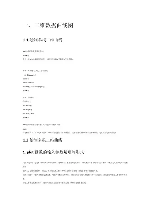
一、二维数据曲线图1.1绘制单根二维曲线plot函数的基本调用格式为：plot(x,y)其中x和y为长度相同的向量，分别用于存储x坐标和y坐标数据。

例1-1在0x2p区间内，绘制曲线y=2e-0.5xcos(4x)程序如下：x=0:pi/100:2*pi;y=2*exp(-0.5*x).*cos(4*pi*x);plot(x,y)例1-2绘制曲线。

程序如下：t=0:0.1:2*pi;x=t.*sin(3*t);y=t.*sin(t).*sin(t);plot(x,y);plot函数最简单的调用格式是只包含一个输入参数：plot(x)在这种情况下，当x是实向量时，以该向量元素的下标为横坐标，元素值为纵坐标画出一条连续曲线，这实际上是绘制折线图。

1.2绘制多根二维曲线1.plot函数的输入参数是矩阵形式(1)当x是向量，y是有一维与x同维的矩阵时，则绘制出多根不同颜色的曲线。

曲线条数等于y矩阵的另一维数，x被作为这些曲线共同的横坐标。

(2)当x,y是同维矩阵时，则以x,y对应列元素为横、纵坐标分别绘制曲线，曲线条数等于矩阵的列数。

(3)对只包含一个输入参数的plot函数，当输入参数是实矩阵时，则按列绘制每列元素值相对其下标的曲线，曲线条数等于输入参数矩阵的列数。

当输入参数是复数矩阵时，则按列分别以元素实部和虚部为横、纵坐标绘制多条曲线。

2含多个输入参数的plot函数调用格式为：plot(x1,y1,x2,y2,,xn,yn)(1)当输入参数都为向量时，x1和yl,x2和y2,,xn和yn分别组成一组向量对，每一组向量对的长度可以不同。

每一向量对可以绘制出一条曲线，这样可以在同一坐标内绘制出多条曲线。

(2)当输入参数有矩阵形式时，配对的x,y按对应列元素为横、纵坐标分别绘制曲线，曲线条数等于矩阵的列数。

例1-3分析下列程序绘制的曲线。

x1=linspace(0,2*pi,100);x2=linspace(0,3*pi,100);x3=linspace(0,4*pi,100);y1=sin(x1);y2=1+sin(x2);y3=2+sin(x3);x=[x1;x2;x3]';y=[y1;y2;y3]';plot(x,y,x1,y1-1)3.具有两个纵坐标标度的图形在MATLAB中，如果需要绘制出具有不同纵坐标标度的两个图形，可以使用plotyy绘图函数。

强大的绘图功能是Matlab的特点之一，Matlab提供了一系列的绘图函数，用户不需要过多的考虑绘图的细节，只需要给出一些基本参数就能得到所需图形，这类函数称为高层绘图函数。

此外，Matlab还提供了直接对图形句柄进行操作的低层绘图操作。

这类操作将图形的每个图形元素（如坐标轴、曲线、文字等）看做一个独立的对象，系统给每个对象分配一个句柄，可以通过句柄对该图形元素进行操作，而不影响其他部分。

本章介绍绘制二维和三维图形的高层绘图函数以及其他图形控制函数的使用方法，在此基础上，再介绍可以操作和控制各种图形对象的低层绘图操作。

一．二维绘图二维图形是将平面坐标上的数据点连接起来的平面图形。

可以采用不同的坐标系，如直角坐标、对数坐标、极坐标等。

二维图形的绘制是其他绘图操作的基础。

一．绘制二维曲线的基本函数在Matlab中，最基本而且应用最为广泛的绘图函数为plot，利用它可以在二维平面上绘制出不同的曲线。

1．plot函数的基本用法plot函数用于绘制二维平面上的线性坐标曲线图，要提供一组x坐标和对应的y坐标，可以绘制分别以x和y为横、纵坐标的二维曲线。

plot函数的应用格式plot(x,y) 其中x,y为长度相同的向量，存储x坐标和y坐标。

例51 在[0 , 2pi]区间，绘制曲线程序如下：在命令窗口中输入以下命令>> x=0:pi/100:2*pi;>> y=2*exp(-0.5*x).*sin(2*pi*x);>> plot(x,y)程序执行后，打开一个图形窗口，在其中绘制出如下曲线注意：指数函数和正弦函数之间要用点乘运算，因为二者是向量。

例52 绘制曲线这是以参数形式给出的曲线方程，只要给定参数向量，再分别求出x,y向量即可输出曲线：>> t=-pi:pi/100:pi;>> x=t.*cos(3*t);>> y=t.*sin(t).*sin(t);>> plot(x,y)程序执行后，打开一个图形窗口，在其中绘制出如下曲线以上提到plot函数的自变量x,y为长度相同的向量，这是最常见、最基本的用法。