CV_Rajan Tulsi12082011[1]

A review on time series data miningTak-chung FuDepartment of Computing,Hong Kong Polytechnic University,Hunghom,Kowloon,Hong Konga r t i c l e i n f oArticle history:Received19February2008Received in revised form14March2010Accepted4September2010Keywords:Time series data miningRepresentationSimilarity measureSegmentationVisualizationa b s t r a c tTime series is an important class of temporal data objects and it can be easily obtained from scientificandfinancial applications.A time series is a collection of observations made chronologically.The natureof time series data includes:large in data size,high dimensionality and necessary to updatecontinuously.Moreover time series data,which is characterized by its numerical and continuousnature,is always considered as a whole instead of individual numericalfield.The increasing use of timeseries data has initiated a great deal of research and development attempts in thefield of data mining.The abundant research on time series data mining in the last decade could hamper the entry ofinterested researchers,due to its complexity.In this paper,a comprehensive revision on the existingtime series data mining researchis given.They are generally categorized into representation andindexing,similarity measure,segmentation,visualization and mining.Moreover state-of-the-artresearch issues are also highlighted.The primary objective of this paper is to serve as a glossary forinterested researchers to have an overall picture on the current time series data mining developmentand identify their potential research direction to further investigation.&2010Elsevier Ltd.All rights reserved.1.IntroductionRecently,the increasing use of temporal data,in particulartime series data,has initiated various research and developmentattempts in thefield of data mining.Time series is an importantclass of temporal data objects,and it can be easily obtained fromscientific andfinancial applications(e.g.electrocardiogram(ECG),daily temperature,weekly sales totals,and prices of mutual fundsand stocks).A time series is a collection of observations madechronologically.The nature of time series data includes:large indata size,high dimensionality and update continuously.Moreovertime series data,which is characterized by its numerical andcontinuous nature,is always considered as a whole instead ofindividual numericalfield.Therefore,unlike traditional databaseswhere similarity search is exact match based,similarity search intime series data is typically carried out in an approximatemanner.There are various kinds of time series data related research,forexample,finding similar time series(Agrawal et al.,1993a;Berndtand Clifford,1996;Chan and Fu,1999),subsequence searching intime series(Faloutsos et al.,1994),dimensionality reduction(Keogh,1997b;Keogh et al.,2000)and segmentation(Abonyiet al.,2005).Those researches have been studied in considerabledetail by both database and pattern recognition communities fordifferent domains of time series data(Keogh and Kasetty,2002).In the context of time series data mining,the fundamentalproblem is how to represent the time series data.One of thecommon approaches is transforming the time series to anotherdomain for dimensionality reduction followed by an indexingmechanism.Moreover similarity measure between time series ortime series subsequences and segmentation are two core tasksfor various time series mining tasks.Based on the time seriesrepresentation,different mining tasks can be found in theliterature and they can be roughly classified into fourfields:pattern discovery and clustering,classification,rule discovery andsummarization.Some of the research concentrates on one of thesefields,while the others may focus on more than one of the aboveprocesses.In this paper,a comprehensive review on the existingtime series data mining research is given.Three state-of-the-arttime series data mining issues,streaming,multi-attribute timeseries data and privacy are also briefly introduced.The remaining part of this paper is organized as follows:Section2contains a discussion of time series representation andindexing.The concept of similarity measure,which includes bothwhole time series and subsequence matching,based on the rawtime series data or the transformed domain will be reviewed inSection3.The research work on time series segmentation andvisualization will be discussed in Sections4and5,respectively.InSection6,vary time series data mining tasks and recent timeseries data mining directions will be reviewed,whereas theconclusion will be made in Section7.2.Time series representation and indexingOne of the major reasons for time series representation is toreduce the dimension(i.e.the number of data point)of theContents lists available at ScienceDirectjournal homepage:/locate/engappaiEngineering Applications of Artificial Intelligence0952-1976/$-see front matter&2010Elsevier Ltd.All rights reserved.doi:10.1016/j.engappai.2010.09.007E-mail addresses:cstcfu@.hk,cstcfu@Engineering Applications of Artificial Intelligence24(2011)164–181original data.The simplest method perhaps is sampling(Astrom, 1969).In this method,a rate of m/n is used,where m is the length of a time series P and n is the dimension after dimensionality reduction(Fig.1).However,the sampling method has the drawback of distorting the shape of sampled/compressed time series,if the sampling rate is too low.An enhanced method is to use the average(mean)value of each segment to represent the corresponding set of data points. Again,with time series P¼ðp1,...,p mÞand n is the dimension after dimensionality reduction,the‘‘compressed’’time series ^P¼ð^p1,...,^p nÞcan be obtained by^p k ¼1k kX e ki¼s kp ið1Þwhere s k and e k denote the starting and ending data points of the k th segment in the time series P,respectively(Fig.2).That is, using the segmented means to represent the time series(Yi and Faloutsos,2000).This method is also called piecewise aggregate approximation(PAA)by Keogh et al.(2000).1Keogh et al.(2001a) propose an extended version called an adaptive piecewise constant approximation(APCA),in which the length of each segment is notfixed,but adaptive to the shape of the series.A signature technique is proposed by Faloutsos et al.(1997)with similar ideas.Besides using the mean to represent each segment, other methods are proposed.For example,Lee et al.(2003) propose to use the segmented sum of variation(SSV)to represent each segment of the time series.Furthermore,a bit level approximation is proposed by Ratanamahatana et al.(2005)and Bagnall et al.(2006),which uses a bit to represent each data point.To reduce the dimension of time series data,another approach is to approximate a time series with straight lines.Two major categories are involved.Thefirst one is linear interpolation.A common method is using piecewise linear representation(PLR)2 (Keogh,1997b;Keogh and Smyth,1997;Smyth and Keogh,1997). The approximating line for the subsequence P(p i,y,p j)is simply the line connecting the data points p i and p j.It tends to closely align the endpoint of consecutive segments,giving the piecewise approximation with connected lines.PLR is a bottom-up algo-rithm.It begins with creating afine approximation of the time series,so that m/2segments are used to approximate the m length time series and iteratively merges the lowest cost pair of segments,until it meets the required number of segment.When the pair of adjacent segments S i and S i+1are merged,the cost of merging the new segment with its right neighbor and the cost of merging the S i+1segment with its new larger neighbor is calculated.Ge(1998)extends PLR to hierarchical structure. Furthermore,Keogh and Pazzani enhance PLR by considering weights of the segments(Keogh and Pazzani,1998)and relevance feedback from the user(Keogh and Pazzani,1999).The second approach is linear regression,which represents the subsequences with the bestfitting lines(Shatkay and Zdonik,1996).Furthermore,reducing the dimension by preserving the salient points is a promising method.These points are called as perceptually important points(PIP).The PIP identification process isfirst introduced by Chung et al.(2001)and used for pattern matching of technical(analysis)patterns infinancial applications. With the time series P,there are n data points:P1,P2y,P n.All the data points in P can be reordered by its importance by going through the PIP identification process.Thefirst data point P1and the last data point P n in the time series are thefirst and two PIPs, respectively.The next PIP that is found will be the point in P with maximum distance to thefirst two PIPs.The fourth PIP that is found will be the point in P with maximum vertical distance to the line joining its two adjacent PIPs,either in between thefirst and second PIPs or in between the second and the last PIPs.The PIP location process continues until all the points in P are attached to a reordered list L or the required number of PIPs is reached(i.e. reduced to the required dimension).Seven PIPs are identified in from the sample time series in Fig.3.Detailed treatment can be found in Fu et al.(2008c).The idea is similar to a technique proposed about30years ago for reducing the number of points required to represent a line by Douglas and Peucker(1973)(see also Hershberger and Snoeyink, 1992).Perng et al.(2000)use a landmark model to identify the important points in the time series for similarity measure.Man and Wong(2001)propose a lattice structure to represent the identified peaks and troughs(called control points)in the time series.Pratt and Fink(2002)and Fink et al.(2003)define extrema as minima and maxima in a time series and compress thetime Fig.1.Time series dimensionality reduction by sampling.The time series on the left is sampled regularly(denoted by dotted lines)and displayed on the right with a largedistortion.Fig.2.Time series dimensionality reduction by PAA.The horizontal dotted lines show the mean of each segment.1This method is called piecewise constant approximation originally(Keoghand Pazzani,2000a).2It is also called piecewise linear approximation(PLA).Tak-chung Fu/Engineering Applications of Artificial Intelligence24(2011)164–181165series by selecting only certain important extrema and dropping the other points.The idea is to discard minor fluctuations and keep major minima and maxima.The compression is controlled by the compression ratio with parameter R ,which is always greater than one;an increase of R leads to the selection of fewer points.That is,given indices i and j ,where i r x r j ,a point p x of a series P is an important minimum if p x is the minimum among p i ,y ,p j ,and p i /p x Z R and p j /p x Z R .Similarly,p x is an important maximum if p x is the maximum among p i ,y ,p j and p x /p i Z R and p x /p j Z R .This algorithm takes linear time and constant memory.It outputs the values and indices of all important points,as well as the first and last point of the series.This algorithm can also process new points as they arrive,without storing the original series.It identifies important points based on local information of each segment (subsequence)of time series.Recently,a critical point model (CPM)(Bao,2008)and a high-level representation based on a sequence of critical points (Bao and Yang,2008)are proposed for financial data analysis.On the other hand,special points are introduced to restrict the error on PLR (Jia et al.,2008).Key points are suggested to represent time series in (Leng et al.,2009)for an anomaly detection.Another common family of time series representation approaches converts the numeric time series to symbolic form.That is,first discretizing the time series into segments,then converting each segment into a symbol (Yang and Zhao,1998;Yang et al.,1999;Motoyoshi et al.,2002;Aref et al.,2004).Lin et al.(2003;2007)propose a method called symbolic aggregate approximation (SAX)to convert the result from PAA to symbol string.The distribution space (y -axis)is divided into equiprobable regions.Each region is represented by a symbol and each segment can then be mapped into a symbol corresponding to the region inwhich it resides.The transformed time series ^Pusing PAA is finally converted to a symbol string SS (s 1,y ,s W ).In between,two parameters must be specified for the conversion.They are the length of subsequence w and alphabet size A (number of symbols used).Besides using the means of the segments to build the alphabets,another method uses the volatility change to build the alphabets.Jonsson and Badal (1997)use the ‘‘Shape Description Alphabet (SDA)’’.Example symbols like highly increasing transi-tion,stable transition,and slightly decreasing transition are adopted.Qu et al.(1998)use gradient alphabets like upward,flat and download as symbols.Huang and Yu (1999)suggest transforming the time series to symbol string,using change ratio between contiguous data points.Megalooikonomou et al.(2004)propose to represent each segment by a codeword from a codebook of key-sequences.This work has extended to multi-resolution consideration (Megalooi-konomou et al.,2005).Morchen and Ultsch (2005)propose an unsupervised discretization process based on quality score and persisting states.Instead of ignoring the temporal order of values like many other methods,the Persist algorithm incorporates temporal information.Furthermore,subsequence clustering is a common method to generate the symbols (Das et al.,1998;Li et al.,2000a;Hugueney and Meunier,2001;Hebrail and Hugueney,2001).A multiple abstraction level mining (MALM)approach is proposed by Li et al.(1998),which is based on the symbolic form of the time series.The symbols in this paper are determined by clustering the features of each segment,such as regression coefficients,mean square error and higher order statistics based on the histogram of the regression residuals.Most of the methods described so far are representing time series in time domain directly.Representing time series in the transformation domain is another large family of approaches.One of the popular transformation techniques in time series data mining is the discrete Fourier transforms (DFT),since first being proposed for use in this context by Agrawal et al.(1993a).Rafiei and Mendelzon (2000)develop similarity-based queries,using DFT.Janacek et al.(2005)propose to use likelihood ratio statistics to test the hypothesis of difference between series instead of an Euclidean distance in the transformed domain.Recent research uses wavelet transform to represent time series (Struzik and Siebes,1998).In between,the discrete wavelet transform (DWT)has been found to be effective in replacing DFT (Chan and Fu,1999)and the Haar transform is always selected (Struzik and Siebes,1999;Wang and Wang,2000).The Haar transform is a series of averaging and differencing operations on a time series (Chan and Fu,1999).The average and difference between every two adjacent data points are computed.For example,given a time series P ¼(1,3,7,5),dimension of 4data points is the full resolution (i.e.original time series);in dimension of two coefficients,the averages are (26)with the coefficients (À11)and in dimension of 1coefficient,the average is 4with coefficient (À2).A multi-level representation of the wavelet transform is proposed by Shahabi et al.(2000).Popivanov and Miller (2002)show that a large class of wavelet transformations can be used for time series representation.Dasha et al.(2007)compare different wavelet feature vectors.On the other hand,comparison between DFT and DWT can be found in Wu et al.(2000b)and Morchen (2003)and a combination use of Fourier and wavelet transforms are presented in Kawagoe and Ueda (2002).An ensemble-index,is proposed by Keogh et al.(2001b)and Vlachos et al.(2006),which ensembles two or more representations for indexing.Principal component analysis (PCA)is a popular multivariate technique used for developing multivariate statistical process monitoring methods (Yang and Shahabi,2005b;Yoon et al.,2005)and it is applied to analyze financial time series by Lesch et al.(1999).In most of the related works,PCA is used to eliminate the less significant components or sensors and reduce the data representation only to the most significant ones and to plot the data in two dimensions.The PCA model defines linear hyperplane,it can be considered as the multivariate extension of the PLR.PCA maps the multivariate data into a lower dimensional space,which is useful in the analysis and visualization of correlated high-dimensional data.Singular value decomposition (SVD)(Korn et al.,1997)is another transformation-based approach.Other time series representation methods include modeling time series using hidden markov models (HMMs)(Azzouzi and Nabney,1998)and a compression technique for multiple stream is proposed by Deligiannakis et al.(2004).It is based onbaseFig.3.Time series compression by data point importance.The time series on the left is represented by seven PIPs on the right.Tak-chung Fu /Engineering Applications of Artificial Intelligence 24(2011)164–181166signal,which encodes piecewise linear correlations among the collected data values.In addition,a recent biased dimension reduction technique is proposed by Zhao and Zhang(2006)and Zhao et al.(2006).Moreover many of the representation schemes described above are incorporated with different indexing methods.A common approach is adopted to an existing multidimensional indexing structure(e.g.R-tree proposed by Guttman(1984))for the representation.Agrawal et al.(1993a)propose an F-index, which adopts the R*-tree(Beckmann et al.,1990)to index thefirst few DFT coefficients.An ST-index is further proposed by (Faloutsos et al.(1994),which extends the previous work for subsequence handling.Agrawal et al.(1995a)adopt both the R*-and R+-tree(Sellis et al.,1987)as the indexing structures.A multi-level distance based index structure is proposed(Yang and Shahabi,2005a),which for indexing time series represented by PCA.Vlachos et al.(2005a)propose a Multi-Metric(MM)tree, which is a hybrid indexing structure on Euclidean and periodic spaces.Minimum bounding rectangle(MBR)is also a common technique for time series indexing(Chu and Wong,1999;Vlachos et al.,2003).An MBR is adopted in(Rafiei,1999)which an MT-index is developed based on the Fourier transform and in(Kahveci and Singh,2004)which a multi-resolution index is proposed based on the wavelet transform.Chen et al.(2007a)propose an indexing mechanism for PLR representation.On the other hand, Kim et al.(1996)propose an index structure called TIP-index (TIme series Pattern index)for manipulating time series pattern databases.The TIP-index is developed by improving the extended multidimensional dynamic indexfile(EMDF)(Kim et al.,1994). An iSAX(Shieh and Keogh,2009)is proposed to index massive time series,which is developed based on an SAX.A multi-resolution indexing structure is proposed by Li et al.(2004),which can be adapted to different representations.To sum up,for a given index structure,the efficiency of indexing depends only on the precision of the approximation in the reduced dimensionality space.However in choosing a dimensionality reduction technique,we cannot simply choose an arbitrary compression algorithm.It requires a technique that produces an indexable representation.For example,many time series can be efficiently compressed by delta encoding,but this representation does not lend itself to indexing.In contrast,SVD, DFT,DWT and PAA all lend themselves naturally to indexing,with each eigenwave,Fourier coefficient,wavelet coefficient or aggregate segment map onto one dimension of an index tree. Post-processing is then performed by computing the actual distance between sequences in the time domain and discarding any false matches.3.Similarity measureSimilarity measure is of fundamental importance for a variety of time series analysis and data mining tasks.Most of the representation approaches discussed in Section2also propose the similarity measure method on the transformed representation scheme.In traditional databases,similarity measure is exact match based.However in time series data,which is characterized by its numerical and continuous nature,similarity measure is typically carried out in an approximate manner.Consider the stock time series,one may expect having queries like: Query1:find all stocks which behave‘‘similar’’to stock A.Query2:find all‘‘head and shoulders’’patterns last for a month in the closing prices of all high-tech stocks.The query results are expected to provide useful information for different stock analysis activities.Queries like Query2in fact is tightly coupled with the patterns frequently used in technical analysis, e.g.double top/bottom,ascending triangle,flag and rounded top/bottom.In time series domain,devising an appropriate similarity function is by no means trivial.There are essentially two ways the data that might be organized and processed(Agrawal et al., 1993a).In whole sequence matching,the whole length of all time series is considered during the similarity search.It requires comparing the query sequence to each candidate series by evaluating the distance function and keeping track of the sequence with the smallest distance.In subsequence matching, where a query sequence Q and a longer sequence P are given,the task is tofind the subsequences in P,which matches Q. Subsequence matching requires that the query sequence Q be placed at every possible offset within the longer sequence P.With respect to Query1and Query2above,they can be considered as a whole sequence matching and a subsequence matching,respec-tively.Gavrilov et al.(2000)study the usefulness of different similarity measures for clustering similar stock time series.3.1.Whole sequence matchingTo measure the similarity/dissimilarity between two time series,the most popular approach is to evaluate the Euclidean distance on the transformed representation like the DFT coeffi-cients(Agrawal et al.,1993a)and the DWT coefficients(Chan and Fu,1999).Although most of these approaches guarantee that a lower bound of the Euclidean distance to the original data, Euclidean distance is not always being the suitable distance function in specified domains(Keogh,1997a;Perng et al.,2000; Megalooikonomou et al.,2005).For example,stock time series has its own characteristics over other time series data(e.g.data from scientific areas like ECG),in which the salient points are important.Besides Euclidean-based distance measures,other distance measures can easily be found in the literature.A constraint-based similarity query is proposed by Goldin and Kanellakis(1995), which extended the work of(Agrawal et al.,1993a).Das et al. (1997)apply computational geometry methods for similarity measure.Bozkaya et al.(1997)use a modified edit distance function for time series matching and retrieval.Chu et al.(1998) propose to measure the distance based on the slopes of the segments for handling amplitude and time scaling problems.A projection algorithm is proposed by Lam and Wong(1998).A pattern recognition method is proposed by Morrill(1998),which is based on the building blocks of the primitives of the time series. Ruspini and Zwir(1999)devote an automated identification of significant qualitative features of complex objects.They propose the process of discovery and representation of interesting relations between those features,the generation of structured indexes and textual annotations describing features and their relations.The discovery of knowledge by an analysis of collections of qualitative descriptions is then achieved.They focus on methods for the succinct description of interesting features lying in an effective frontier.Generalized clustering is used for extracting features,which interest domain experts.The general-ized Markov models are adopted for waveform matching in Ge and Smyth(2000).A content-based query-by-example retrieval model called FALCON is proposed by Wu et al.(2000a),which incorporates a feedback mechanism.Indeed,one of the most popular andfield-tested similarity measures is called the‘‘time warping’’distance measure.Based on the dynamic time warping(DTW)technique,the proposed method in(Berndt and Clifford,1994)predefines some patterns to serve as templates for the purpose of pattern detection.To align two time series,P and Q,using DTW,an n-by-m matrix M isfirstTak-chung Fu/Engineering Applications of Artificial Intelligence24(2011)164–181167constructed.The(i th,j th)element of the matrix,m ij,contains the distance d(q i,p j)between the two points q i and p j and an Euclidean distance is typically used,i.e.d(q i,p j)¼(q iÀp j)2.It corresponds to the alignment between the points q i and p j.A warping path,W,is a contiguous set of matrix elements that defines a mapping between Q and P.Its k th element is defined as w k¼(i k,j k)andW¼w1,w2,...,w k,...,w Kð2Þwhere maxðm,nÞr K o mþnÀ1.The warping path is typically subjected to the following constraints.They are boundary conditions,continuity and mono-tonicity.Boundary conditions are w1¼(1,1)and w K¼(m,n).This requires the warping path to start andfinish diagonally.Next constraint is continuity.Given w k¼(a,b),then w kÀ1¼(a0,b0), where aÀa u r1and bÀb u r1.This restricts the allowable steps in the warping path being the adjacent cells,including the diagonally adjacent cell.Also,the constraints aÀa uZ0and bÀb uZ0force the points in W to be monotonically spaced in time.There is an exponential number of warping paths satisfying the above conditions.However,only the path that minimizes the warping cost is of interest.This path can be efficiently found by using dynamic programming(Berndt and Clifford,1996)to evaluate the following recurrence equation that defines the cumulative distance gði,jÞas the distance dði,jÞfound in the current cell and the minimum of the cumulative distances of the adjacent elements,i.e.gði,jÞ¼dðq i,p jÞþmin f gðiÀ1,jÀ1Þ,gðiÀ1,jÞ,gði,jÀ1Þgð3ÞA warping path,W,such that‘‘distance’’between them is minimized,can be calculated by a simple methodDTWðQ,PÞ¼minWX Kk¼1dðw kÞ"#ð4Þwhere dðw kÞcan be defined asdðw kÞ¼dðq ik ,p ikÞ¼ðq ikÀp ikÞ2ð5ÞDetailed treatment can be found in Kruskall and Liberman (1983).As DTW is computationally expensive,different methods are proposed to speedup the DTW matching process.Different constraint(banding)methods,which control the subset of matrix that the warping path is allowed to visit,are reviewed in Ratanamahatana and Keogh(2004).Yi et al.(1998)introduce a technique for an approximate indexing of DTW that utilizes a FastMap technique,whichfilters the non-qualifying series.Kim et al.(2001)propose an indexing approach under DTW similarity measure.Keogh and Pazzani(2000b)introduce a modification of DTW,which integrates with PAA and operates on a higher level abstraction of the time series.An exact indexing approach,which is based on representing the time series by PAA for DTW similarity measure is further proposed by Keogh(2002).An iterative deepening dynamic time warping(IDDTW)is suggested by Chu et al.(2002),which is based on a probabilistic model of the approximate errors for all levels of approximation prior to the query process.Chan et al.(2003)propose afiltering process based on the Haar wavelet transformation from low resolution approx-imation of the real-time warping distance.Shou et al.(2005)use an APCA approximation to compute the lower bounds for DTW distance.They improve the global bound proposed by Kim et al. (2001),which can be used to index the segments and propose a multi-step query processing technique.A FastDTW is proposed by Salvador and Chan(2004).This method uses a multi-level approach that recursively projects a solution from a coarse resolution and refines the projected solution.Similarly,a fast DTW search method,an FTW is proposed by Sakurai et al.(2005) for efficiently pruning a significant number of search candidates. Ratanamahatana and Keogh(2005)clarified some points about DTW where are related to lower bound and speed.Euachongprasit and Ratanamahatana(2008)also focus on this problem.A sequentially indexed structure(SIS)is proposed by Ruengron-ghirunya et al.(2009)to balance the tradeoff between indexing efficiency and I/O cost during DTW similarity measure.A lower bounding function for group of time series,LBG,is adopted.On the other hand,Keogh and Pazzani(2001)point out the potential problems of DTW that it can lead to unintuitive alignments,where a single point on one time series maps onto a large subsection of another time series.Also,DTW may fail to find obvious and natural alignments in two time series,because of a single feature(i.e.peak,valley,inflection point,plateau,etc.). One of the causes is due to the great difference between the lengths of the comparing series.Therefore,besides improving the performance of DTW,methods are also proposed to improve an accuracy of DTW.Keogh and Pazzani(2001)propose a modifica-tion of DTW that considers the higher level feature of shape for better alignment.Ratanamahatana and Keogh(2004)propose to learn arbitrary constraints on the warping path.Regression time warping(RTW)is proposed by Lei and Govindaraju(2004)to address the challenges of shifting,scaling,robustness and tecki et al.(2005)propose a method called the minimal variance matching(MVM)for elastic matching.It determines a subsequence of the time series that best matches a query series byfinding the cheapest path in a directed acyclic graph.A segment-wise time warping distance(STW)is proposed by Zhou and Wong(2005)for time scaling search.Fu et al.(2008a) propose a scaled and warped matching(SWM)approach for handling both DTW and uniform scaling simultaneously.Different customized DTW techniques are applied to thefield of music research for query by humming(Zhu and Shasha,2003;Arentz et al.,2005).Focusing on similar problems as DTW,the Longest Common Subsequence(LCSS)model(Vlachos et al.,2002)is proposed.The LCSS is a variation of the edit distance and the basic idea is to match two sequences by allowing them to stretch,without rearranging the sequence of the elements,but allowing some elements to be unmatched.One of the important advantages of an LCSS over DTW is the consideration on the outliers.Chen et al.(2005a)further introduce a distance function based on an edit distance on real sequence(EDR),which is robust against the data imperfection.Morse and Patel(2007)propose a Fast Time Series Evaluation(FTSE)method which can be used to evaluate the threshold value of these kinds of techniques in a faster way.Threshold-based distance functions are proposed by ABfalg et al. (2006).The proposed function considers intervals,during which the time series exceeds a certain threshold for comparing time series rather than using the exact time series values.A T-Time application is developed(ABfalg et al.,2008)to demonstrate the usage of it.Fu et al.(2007)further suggest to introduce rules to govern the pattern matching process,if a priori knowledge exists in the given domain.A parameter-light distance measure method based on Kolmo-gorov complexity theory is suggested in Keogh et al.(2007b). Compression-based dissimilarity measure(CDM)3is adopted in this paper.Chen et al.(2005b)present a histogram-based representation for similarity measure.Similarly,a histogram-based similarity measure,bag-of-patterns(BOP)is proposed by Lin and Li(2009).The frequency of occurrences of each pattern in 3CDM is proposed by Keogh et al.(2004),which is used to compare the co-compressibility between data sets.Tak-chung Fu/Engineering Applications of Artificial Intelligence24(2011)164–181 168。

Journal of Machine Learning Research15(2014)3183-3186Submitted6/12;Revised6/13;Published10/14ooDACE Toolbox:A Flexible Object-Oriented Kriging ImplementationIvo Couckuyt∗********************* Tom Dhaene******************* Piet Demeester*********************** Ghent University-iMindsDepartment of Information Technology(INTEC)Gaston Crommenlaan89050Gent,BelgiumEditor:Mikio BraunAbstractWhen analyzing data from computationally expensive simulation codes,surrogate model-ing methods arefirmly established as facilitators for design space exploration,sensitivity analysis,visualization and optimization.Kriging is a popular surrogate modeling tech-nique used for the Design and Analysis of Computer Experiments(DACE).Hence,the past decade Kriging has been the subject of extensive research and many extensions have been proposed,e.g.,co-Kriging,stochastic Kriging,blind Kriging,etc.However,few Krig-ing implementations are publicly available and tailored towards scientists and engineers.Furthermore,no Kriging toolbox exists that unifies several Krigingflavors.This paper addresses this need by presenting an efficient object-oriented Kriging implementation and several Kriging extensions,providing aflexible and easily extendable framework to test and implement new Krigingflavors while reusing as much code as possible.Keywords:Kriging,Gaussian process,co-Kriging,blind Kriging,surrogate modeling, metamodeling,DACE1.IntroductionThis paper is concerned with efficiently solving complex,computational expensive problems using surrogate modeling techniques(Gorissen et al.,2010).Surrogate models,also known as metamodels,are cheap approximation models for computational expensive(black-box) simulations.Surrogate modeling techniques are well-suited to handle,for example,expen-sivefinite element(FE)simulations and computationalfluid dynamic(CFD)simulations.Kriging is a popular surrogate model type to approximate deterministic noise-free data. First conceived by Danie Krige in geostatistics and later introduced for the Design and Analysis of Computer Experiments(DACE)by Sacks et al.(1989),these Gaussian pro-cess(Rasmussen and Williams,2006)based surrogate models are compact and cheap to evaluate,and have proven to be very useful for tasks such as optimization,design space exploration,visualization,prototyping,and sensitivity analysis(Viana et al.,2014).Note ∗.Ivo Couckuyt is a post-doctoral research fellow of FWO-Vlaanderen.Couckuyt,Dhaene and Demeesterthat Kriging surrogate models are primarily known as Gaussian processes in the machine learning community.Except for the utilized terminology there is no difference between the terms and associated methodologies.While Kriging is a popular surrogate model type,not many publicly available,easy-to-use Kriging implementations exist.Many Kriging implementations are outdated and often limited to one specific type of Kriging.Perhaps the most well-known Kriging toolbox is the DACE toolbox1of Lophaven et al.(2002),but,unfortunately,the toolbox has not been updated for some time and only the standard Kriging model is provided.Other freely available Kriging codes include:stochastic Kriging(Staum,2009),2DiceKriging,3 Gaussian processes for Machine Learning(Rasmussen and Nickisch,2010)(GPML),4demo code provided with Forrester et al.(2008),5and the Matlab Krigeage toolbox.6 This paper addresses this need by presenting an object-oriented Kriging implementation and several Kriging extensions,providing aflexible and easily extendable framework to test and implement new Krigingflavors while reusing as much code as possible.2.ooDACE ToolboxThe ooDACE toolbox is an object-oriented Matlab toolbox implementing a variety of Krig-ingflavors and extensions.The most important features and Krigingflavors include:•Simple Kriging,ordinary Kriging,universal Kriging,stochastic Kriging(regression Kriging),blind-and co-Kriging.•Derivatives of the prediction and prediction variance.•Flexible hyperparameter optimization.•Useful utilities include:cross-validation,integrated mean squared error,empirical variogram plot,debug plot of the likelihood surface,robustness-criterion value,etc.•Proper object-oriented design(compatible interface with the DACE toolbox1is avail-able).Documentation of the ooDACE toolbox is provided in the form of a getting started guide (for users),a wiki7and doxygen documentation8(for developers and more advanced users). In addition,the code is well-documented,providing references to research papers where appropriate.A quick-start demo script is provided withfive surrogate modeling use cases, as well as script to run a suite of regression tests.A simplified UML class diagram,showing only the most important public operations, of the toolbox is shown in Figure1.The toolbox is designed with efficiency andflexibil-ity in mind.The process of constructing(and predicting)a Kriging model is decomposed in several smaller,logical steps,e.g.,constructing the correlation matrix,constructing the1.The DACE toolbox can be downloaded at http://www2.imm.dtu.dk/~hbn/dace/.2.The stochastic Kriging toolbox can be downloaded at /.3.The DiceKriging toolbox can be downloaded at /web/packages/DiceKriging/index.html.4.The GPML toolbox can be downloaded at /software/view/263/.5.Demo code of Kriging can be downloaded at //legacy/wileychi/forrester/.6.The Krigeage toolbox can be downloaded at /software/kriging/.7.The wiki documentation of the ooDACE toolbox is found at http://sumowiki.intec.ugent.be/index.php/ooDACE:ooDACE_toolbox.8.The doxygen documentation of the ooDACE toolbox is found at http://sumo.intec.ugent.be/buildbot/ooDACE/doc/.Figure1:Class diagram of the ooDACE toolbox.regression matrix,updating the model,optimizing the parameters,etc.These steps are linked together by higher-level steps,e.g.,fitting the Kriging model and making predic-tions.The basic steps needed for Kriging are implemented as(protected)operations in the BasicGaussianProcess superclass.Implementing a new Kriging type,or extending an existing one,is now done by subclassing the Kriging class of your choice and inheriting the(protected)methods that need to be reimplemented.Similarly,to implement a new hyperparameter optimization strategy it suffices to create a new class inherited from the Optimizer class.To assess the performance of the ooDACE toolbox a comparison between the ooDACE toolbox and the DACE toolbox1is performed using the2D Branin function.To that end,20data sets of increasing size are constructed,each drawn from an uniform random distribution.The number of observations ranges from10to200samples with steps of10 samples.For each data set,a DACE toolbox1model,a ooDACE ordinary Kriging and a ooDACE blind Kriging model have been constructed and the accuracy is measured on a dense test set using the Average Euclidean Error(AEE).Moreover,each test is repeated 1000times to remove any random factor,hence the average accuracy of all repetitions is used.Results are shown in Figure2a.Clearly,the ordinary Kriging model of the ooDACE toolbox consistently outperforms the DACE toolbox for any given sample size,mostly due to a better hyperparameter optimization,while the blind Kriging model is able improve the accuracy even more.3.ApplicationsThe ooDACE Toolbox has already been applied successfully to a wide range of problems, e.g.,optimization of a textile antenna(Couckuyt et al.,2010),identification of the elasticity of the middle-ear drum(Aernouts et al.,2010),etc.In sum,the ooDACE toolbox aims to provide a modern,up to date Kriging framework catered to scientists and age instructions,design documentation,and stable releases can be found at http://sumo.intec.ugent.be/?q=ooDACE.ReferencesJ.Aernouts,I.Couckuyt,K.Crombecq,and J.J.J.Dirckx.Elastic characterization of membranes with a complex shape using point indentation measurements and inverseCouckuyt,Dhaene and Demeester(a)(b)Figure2:(a)Evolution of the average AEE versus the number of samples(Branin function).(b)Landscape plot of the Branin function.modelling.International Journal of Engineering Science,48:599–611,2010.I.Couckuyt,F.Declercq,T.Dhaene,and H.Rogier.Surrogate-based infill optimization applied to electromagnetic problems.Journal of RF and Microwave Computer-Aided Engineering:Advances in Design Optimization of Microwave/RF Circuits and Systems, 20(5):492–501,2010.A.Forrester,A.Sobester,and A.Keane.Engineering Design Via Surrogate Modelling:A Practical Guide.Wiley,Chichester,2008.D.Gorissen,K.Crombecq,I.Couckuyt,P.Demeester,and T.Dhaene.A surrogate modeling and adaptive sampling toolbox for computer based design.Journal of Machine Learning Research,11:2051–2055,2010.URL http://sumo.intec.ugent.be/.S.N.Lophaven,H.B.Nielsen,and J.Søndergaard.Aspects of the Matlab toolbox DACE. Technical report,Informatics and Mathematical Modelling,Technical University of Den-mark,DTU,Richard Petersens Plads,Building321,DK-2800Kgs.Lyngby,2002.C.E.Rasmussen and H.Nickisch.Gaussian processes for machine learning(GPML)toolbox. Journal of Machine Learning Research,11:3011–3015,2010.C.E.Rasmussen and C.K.I.Williams.Gaussian Processes for Machine Learning.MIT Press,2006.J.Sacks,W.J.Welch,T.J.Mitchell,and H.P.Wynn.Design and analysis of computer experiments.Statistical Science,4(4):409–435,1989.J.Staum.Better simulation metamodeling:The why,what,and how of stochastic Kriging. In Proceedings of the Winter Simulation Conference,2009.F.A.C.Viana,T.W.Simpson,V.Balabanov,and V.Toropov.Metamodeling in multi-disciplinary design optimization:How far have we really come?AIAA Journal,52(4): 670–690,2014.。

HAZOP e Local approach in the Mexican oil &gas industryM.Pérez-Marín a ,M.A.Rodríguez-Toral b ,*aInstituto Mexicano del Petróleo,Dirección de Seguridad y Medio Ambiente,Eje Central Lázaro Cárdenas Norte No.152,07730México,D.F.,Mexicob PEMEX,Dirección Corporativa de Operaciones,Gerencia de Análisis de Inversiones,Torre Ejecutiva,Piso 12,Av.Marina Nacional No.329,11311México,D.F.,Mexicoa r t i c l e i n f oArticle history:Received 3September 2012Received in revised form 26March 2013Accepted 27March 2013Keywords:HAZOPRisk acceptance criteria Oil &gasa b s t r a c tHAZOP (Hazard and Operability)studies began about 40years ago,when the Process Industry and complexity of its operations start to massively grow in different parts of the world.HAZOP has been successfully applied in Process Systems hazard identi fication by operators,design engineers and consulting firms.Nevertheless,after a few decades since its first applications,HAZOP studies are not truly standard in worldwide industrial practice.It is common to find differences in its execution and results format.The aim of this paper is to show that in the Mexican case at National level in the oil and gas industry,there exist an explicit acceptance risk criteria,thus impacting the risk scenarios prioritizing process.Although HAZOP studies in the Mexican oil &gas industry,based on PEMEX corporate standard has precise acceptance criteria,it is not a signi ficant difference in HAZOP applied elsewhere,but has the advantage of being fully transparent in terms of what a local industry is willing to accept as the level of risk acceptance criteria,also helps to gain an understanding of the degree of HAZOP applications in the Mexican oil &gas sector.Contrary to this in HAZOP ISO standard,risk acceptance criteria is not speci fied and it only mentions that HAZOP can consider scenarios ranking.The paper concludes indicating major implications of risk ranking in HAZOP,whether before or after safeguards identi fication.Ó2013Elsevier Ltd.All rights reserved.1.IntroductionHAZOP (Hazard and Operability)studies appeared in systematic way about 40years ago (Lawley,1974)where a multidisciplinary group uses keywords on Process variables to find potential hazards and operability troubles (Mannan,2012,pp.8-31).The basic prin-ciple is to have a full process description and to ask in each node what deviations to the design purpose can occur,what causes produce them,and what consequences can be presented.This is done systematically by applying the guide words:Not ,More than ,Less than ,etc.as to generate a list of potential failures in equipment and process components.The objective of this paper is to show that in the Mexican case at National level in the oil and gas industry,there is an explicit acceptance risk criteria,thus impacting the risk scenarios priori-tizing process.Although HAZOP methodology in the Mexican oil &gas industry,based on PEMEX corporate standard has precise acceptance criteria,it is not a signi ficant difference in HAZOP studies applied elsewhere,but has the advantage of being fullytransparent in terms of what a local industry is willing to accept as the level of risk acceptance criteria,also helps to gain an under-standing of the degree of HAZOP applications in the Mexican oil &gas sector.Contrary to this in HAZOP ISO standard (ISO,2000),risk acceptance criteria is not speci fied and it only mentions that HAZOP can consider scenarios ranking.The paper concludes indicating major implications of risk prioritizing in HAZOP,whether before or after safeguards identi fication.2.Previous workHAZOP studies include from original ICI method with required actions only,to current applications based on computerized documentation,registering design intentions at nodes,guide words,causes,deviations,consequences,safeguards,cause fre-quencies,loss contention impact,risk reduction factors,scenarios analysis,finding analysis and many combinations among them.In the open literature there have been reported interesting and signi ficant studies about HAZOP,like HAZOP and HAZAN differences (Gujar,1996)where HAZOP was identi fied as qualitative hazard identi fication technique,while HAZAN was considered for the quantitative risk determination.This difference is not strictly valid today,since there are now companies using HAZOP with risk analysis*Corresponding author.Tel.:þ525519442500x57043.E-mail addresses:mpmarin@imp.mx (M.Pérez-Marín),miguel.angel.rodriguezt@ ,matoral09@ (M.A.Rodríguez-Toral).Contents lists available at SciVerse ScienceDirectJournal of Loss Prevention in the Process Industriesjou rn al homepage :/locate/jlp0950-4230/$e see front matter Ó2013Elsevier Ltd.All rights reserved./10.1016/j.jlp.2013.03.008Journal of Loss Prevention in the Process Industries 26(2013)936e 940and its acceptance criteria(Goyal&Kugan,2012).Other approaches include HAZOP execution optimization(Khan,1997);the use of intelligent systems to automate HAZOP(Venkatasubramanian,Zhao, &Viswanathan,2000);the integration of HAZOP with Fault Tree Analysis(FTA)and with Event Tree Analysis(ETA)(Kuo,Hsu,& Chang,1997).According to CCPS(2001)any qualitative method for hazard evaluation applied to identify scenarios in terms of their initial causes,events sequence,consequences and safeguards,can beextended to register Layer of Protection Analysis(LOPA).Since HAZOP scenarios report are presented typically in tabular form there can be added columns considering the frequency in terms of order of magnitude and the probability of occurrence identified in LOPA.There should be identified the Independent and the non-Independent Protection Layers,IPL and non-IPL respec-tively.Then the Probability of Failure on Demand(PFDs)for IPL and for non-IPL can be included as well as IPL integrity.Another approach consists of a combination of HAZOP/LOPA analysis including risk magnitude to rank risk reduction actions (Johnson,2010),a general method is shown,without emphasizing in any particular application.An extended HAZOP/LOPA analysis for Safety Integrity Level(SIL)is presented there,showing the quan-titative benefit of applying risk reduction measures.In this way one scenario can be compared with tolerable risk criteria besides of being able to compare each scenario according to its risk value.A recent review paper has reported variations of HAZOP methodology for several applications including batch processes, laboratory operations,mechanical operations and programmable electronic systems(PES)among others(Dunjó,Fthenakis,Vílchez, &Arnaldos,2010).Wide and important contributions to HAZOP knowledge have been reported in the open literature that have promoted usage and knowledge of HAZOP studies.However,even though there is available the IEC standard on HAZOP studies,IEC-61882:2001there is not a worldwide agreement on HAZOP methodology and there-fore there exist a great variety of approaches for HAZOP studies.At international level there exist an ample number of ap-proaches in HAZOP studies;even though the best advanced prac-tices have been taken by several expert groups around the world, there is not uniformity among different consulting companies or industry internal expert groups(Goyal&Kugan,2012).The Mexican case is not the exception about this,but in the local oil and gas industry there exist a national PEMEX corporate standard that is specific in HAZOP application,it includes ranking risk scenarios (PEMEX,2008),qualitative hazard ranking,as well as the two ap-proaches recognized in HAZOP,Cause by Cause(CÂC)and Devia-tion by Deviation(DÂD).Published work including risk criteria include approaches in countries from the Americas,Europe and Asia(CCPS,2009),but nothing about Mexico has been reported.3.HAZOP variationsIn the technical literature there is no consensus in the HAZOP studies procedure,from the several differences it is consider that the more important are the variations according to:(DÂD)or (CÂC).Table1shows HAZOP variations,where(CQÂCQ)means Consequence by Consequence analysis.The implications of choosing(CÂC)are that in this approach there are obtained unique relationships of Consequences,Safeguards and Recommendations,for each specific Cause of a given Deviation. For(DÂD),all Causes,Consequences,Safeguards and Recommenda-tions are related only to one particular Deviation,thus producing that not all Causes appear to produce all the Consequences.In practice HAZOP approach(DÂD)can optimize analysis time development.However,its drawback comes when HAZOP includes risk ranking since it cannot be determined easily which Cause to consider in probability assignment.In choosing(CÂC)HAZOP there is no such a problem,although it may take more time on the analysis.The HAZOP team leader should agree HAZOP approach with customer and communicate this to the HAZOP team.In our experience factors to consider when choosing HAZOP approach are:1.If HAZOP will be followed by Layers of Protection Analysis(LOPA)for Safety Integrity Level(SIL)selection,then choose (CÂC).2.If HAZOP is going to be the only hazard identification study,it isworth to make it with major detail using(CÂC).3.If HAZOP is part of an environmental risk study that requires aConsequence analysis,then use(DÂD).4.If HAZOP is going to be done with limited time or becauseHAZOP team cannot spend too much time in the analysis,then use(DÂD).Although this is not desirable since may compro-mise process safety.Regarding risk ranking in HAZOP,looking at IEC standard(IEC, 2001)it is found that HAZOP studies there are(DÂD)it refers to (IEC,1995)in considering deviation ranking in accordance to their severity or on their relative risk.One advantage of risk ranking is that presentation of HAZOP results is very convenient,in particular when informing the management on the recommendations to be followedfirst or with higher priority as a function of risk evaluated by the HAZOP team regarding associated Cause with a given recommendation.Tables2and3are shown as illustrative example of the convenience of event risk ranking under HAZOP,showing no risk ranking in Table2and risk ranking in Table3.When HAZOP presents a list of recommendations without ranking,the management can focus to recommendations with perhaps the lower resource needs and not necessarily the ones with higher risk.Table1Main approaches in HAZOP studies.Source HAZOP approach(Crowl&Louvar,2011)(DÂD)(ABS,2004)(CÂC)&(DÂD)(Hyatt,2003)(CÂC),(DÂD)&(CQÂCQ) (IEC,2001)(DÂD)(CCPS,2008);(Crawley,Preston,& Tyler,2008)(DÂD),(CÂC)Table2HAZOP recommendations without risk ranking.DescriptionRecommendation1Recommendation2Recommendation3Recommendation4Recommendation5Table3HAZOP recommendations with risk ranking.Scenario risk DescriptionHigh Recommendation2High Recommendation5Medium Recommendation3Low Recommendation1Low Recommendation4M.Pérez-Marín,M.A.Rodríguez-Toral/Journal of Loss Prevention in the Process Industries26(2013)936e940937As can be seen in Tables 2and 3,for the management there will be more important to know HAZOP results as in Table 3,in order to take decisions on planning response according to ranking risk.4.HAZOP standard for the Mexican oil &gas industryLooking at the worldwide recognized guidelines for hazard identi fication (ISO,2000)there is mentioned that when consid-ering scenarios qualitative risk assignment,one may use risk matrix for comparing the importance of risk reduction measures of the different options,but there is not a speci fic risk matrix with risk values to consider.In Mexico there exist two national standards were tolerable and intolerable risk is de fined,one is the Mexican National Standard NOM-028(NOM,2005)and the other is PEMEX corporate standard NRF-018(PEMEX,2008).In both Mexican standards the matrix form is considered for relating frequency and consequences.Fig.1shows the risk matrix in (NOM,2005),nomenclature regarding letters in this matrix is described in Tables 4e 6.It can be mentioned that risk matrix in (NOM,2005)is optional for risk management in local chemical process plants.For Mexican oil &gas industry,there exist a PEMEX corporate standard (NRF),Fig.2,shows the corresponding risk matrix (PEMEX,2008).Nomenclature regarding letters in this matrix is described in Tables 7e 9for risk concerning the community.It is important to mention that PEMEX corporate standard considers environmental risks,business risks,and corporate image risks.These are not shown here for space limitations.The Mexican National Standard (NOM)as being of general applicability gives the possibility for single entities (like PEMEX)to determine its own risk criteria as this company opted to do.PEMEX risk matrix can be converted to NOM ’s by category ’s grouping infrequency categories,thus giving same flexibility,but with risk speci fic for local industry acceptance risk criteria.One principal consideration in ranking risk is to de fine if ranking is done before safeguards de finition or after.This de finition is relevant in:HAZOP kick-off presentation by HAZOP leader,explaining im-plications of risk ranking.HAZOP schedule de finition.Risk ranking at this point takes shorter time since time is not consumed in estimating risk reduction for each safeguard.If after HAZOP a LOPA is going to be done,then it should be advisable to request that HAZOP leader considers risk ranking before safeguards de finition,since LOPA has established rules in de fining which safeguards are protections and the given risk reduction.Otherwise if for time or resource limitations HAZOP is not going to be followed by LOPA,then HAZOP should consider risk ranking after safeguards de finition.Therefore,the HAZOP leader should explain to the HAZOP team at the kick-off meeting a concise explanation of necessary considerations to identify safeguards having criteria to distinguish them as Independent Protection Layers (IPL)as well as the risk reduction provided by each IPL.In HAZOP report there should be make clear all assumptions and credits given to the Protections identi fied by the HAZOP team.Figs.3and 4,shows a vision of both kinds of HAZOP reports:For the case of risk ranking before and after safeguards de finition.In Figs.3Fig.1.Risk matrix in (NOM,2005).Table 5Probability description (Y -axis of matrix in Fig.1)(NOM,2005).Frequency Frequency quantitative criteria L41in 10years L31in 100years L21in 1000years L1<1in 1000yearsTable 6Risk description (within matrix in Fig.1)(NOM,2005).Risk level Risk qualitative descriptionA Intolerable:risk must be reduced.B Undesirable:risk reduction required or a more rigorous risk estimation.C Tolerable risk:risk reduction is needed.DTolerable risk:risk reduction not needed.Fig.2.Risk matrix as in (PEMEX,2008).Table 7Probability description (Y -axis of matrix in Fig.2)(PEMEX,2008).Frequency Occurrence criteria Category Type Quantitative QualitativeHighF4>10À1>1in 10yearsEvent can be presented within the next 10years.Medium F310À1À10À21in 10years e 1in 100years It can occur at least once in facility lifetime.LowF210À2À10À31in 100years e 1in 1000years Possible,it has never occurred in the facility,but probably ithas occurred in a similar facility.Remote F1<10À3<1in 1000years Virtually impossible.It is norealistic its occurrence.Table 4Consequences description (X -axis of matrix in Fig.1)(NOM,2005).Consequences Consequence quantitative criteriaC4One or more fatalities (on site).Injuries or fatalities in the community (off-site).C3Permanent damage in a speci fic Process or construction area.Several disability accidents or hospitalization.C2One disability accident.Multiple injuries.C1One injured.Emergency response without injuries.M.Pérez-Marín,M.A.Rodríguez-Toral /Journal of Loss Prevention in the Process Industries 26(2013)936e 940938and4“F”means frequency,C means consequence and R is risk as a function of“F”and“C”.One disadvantage of risk ranking before safeguards definition is that resulting risks usually are found to be High,Intolerable or Unacceptable.This makes difficult the decision to be made by the management on what recommendations should be carried outfirst and which can wait.One advantage in risk ranking after safeguards definition is that it allows to show the management the risk scenario fully classified, without any tendency for identifying most risk as High(Intolerable or Unacceptable).In this way,the management will have a good description on which scenario need prompt attention and thus take risk to tolerable levels.There is commercial software for HAZOP methodology,but it normally requires the user to use his/her risk matrix,since risk matrix definition represents an extensive knowledge,resources and consensus to be recognized.The Mexican case is worldwide unique in HAZOP methodology, since it uses an agreed and recognized risk matrix and risk priori-tizing criteria according to local culture and risk understanding for the oil&gas sector.The risk matrix with corresponding risk levels took into account political,economical and ethic values.Advantages in using risk matrix in HAZOP are:they are easy to understand and to apply;once they are established and recognized they are of low cost;they allow risk ranking,thus helping risk reduction requirements and limitations.However,some disad-vantages in risk matrix use are:it may sometimes be difficult to separate frequency categories,for instance it may not be easy to separate low from remote in Table7.The risk matrix subdivision may have important uncertainties,because there are qualitative considerations in its definition.Thus,it may be advantageous to update Pemex corporate HAZOP standard(PEMEX,2008)to consider a6Â6matrix instead of the current4Â4matrix.5.ConclusionsHAZOP studies are not a simple procedure application that as-sures safe Process systems on its own.It is part of a global design cycle.Thus,it is necessary to establish beforehand the HAZOP study scope that should include at least:methodology,type(CÂC,DÂD, etc.)report format,acceptance risk criteria and expected results.Mexico belongs to the reduced number of places where accep-tance risk criteria has been explicitly defined for HAZOP studies at national level.ReferencesABS.(2004).Process safety institute.Course103“Process hazard analysis leader training,using the HAZOP and what-if/checklist techniques”.Houston TX:Amer-ican Bureau of Shipping.CCPS(Center for Chemical Process Safety).(2001).Layer of protection analysis: Simplified process risk assessment.New York,USA:AIChE.CCPS(Center for Chemical Process Safety).(2008).Guidelines for hazard evaluation procedures(3rd ed.).New York,USA:AIChE/John Wiley&Sons.CCPS(Center for Chemical Process Safety).(2009).Guidelines for Developing Quan-titative Safety Risk Criteria,Appendix B.Survey of worldwide risk criteria appli-cations.New York,USA:AIChE.Crawley,F.,Preston,M.,&Tyler,B.(2008).HAZOP:Guide to best practice(2nd ed.).UK:Institution of Chemical Engineers.Crowl,D.A.,&Louvar,J.F.(2011).Chemical process safety,fundamentals with ap-plications(3rd ed.).New Jersey,USA:Prentice Hall.Table8Consequences description(X-axis of matrix in Fig.2)(PEMEX,2008).Event type and consequence categoryEffect:Minor C1Moderate C2Serious C3Catastrophic C4 To peopleNeighbors Health and Safety.No impact on publichealth and safety.Neighborhood alert;potentialimpact to public health and safety.Evacuation;Minor injuries or moderateconsequence on public health and safety;side-effects cost between5and10millionMX$(0.38e0.76million US$).Evacuation;injured people;one ormore fatalities;sever consequenceon public health and safety;injuriesand side-consequence cost over10million MX$(0.76million US$).Health and Safetyof employees,serviceproviders/contractors.No injuries;first aid.Medical treatment;Minor injurieswithout disability to work;reversible health treatment.Hospitalization;multiple injured people;total or partial disability;moderate healthtreatment.One o more fatalities;Severe injurieswith irreversible damages;permanenttotal or partial incapacity.Table9Risk description(within matrix in Fig.2)(PEMEX,2008).Risk level Risk description Risk qualitative descriptionA Intolerable Risk requires immediate action;cost should not be a limitation and doing nothing is not an acceptable option.Risk with level“A”represents an emergency situation and there should be implements with immediate temporary controls.Risk mitigation should bedone by engineered controls and/or human factors until Risk is reduced to type“C”or preferably to type“D”in less than90days.B Undesirable Risk should be reduced and there should be additional investigation.However,corrective actions should be taken within the next90days.If solution takes longer there should be installed on-site immediate temporary controls for risk reduction.C Acceptablewith control Significant risk,but can be compensated with corrective actions during programmed facilities shutdown,to avoid interruption of work plans and extra-costs.Solutions measures to solve riskfindings should be done within18months.Mitigation actions should focus operations discipline and protection systems reliability.D ReasonablyacceptableRisk requires control,but it is of low impact and its attention can be carried out along with other operations improvements.Fig.3.Risk ranking before safeguard definition.Fig.4.Risk ranking after safeguards definition.M.Pérez-Marín,M.A.Rodríguez-Toral/Journal of Loss Prevention in the Process Industries26(2013)936e940939Dunjó,J.,Fthenakis,V.,Vílchez,J.A.,&Arnaldos,J.(2010).Hazard and opera-bility(HAZOP)analysis.A literature review.Journal of Hazardous Materials, 173,19e32.Goyal,R.K.,&Kugan,S.(2012).Hazard and operability studies(HAZOP)e best practices adopted by BAPCO(Barahin Petroleum Company).In Presented at SPE middle east health,safety,security and environment conference and exhibition.Abu Dhabi,UAE.2e4April.Gujar,A.M.(1996).Myths of HAZOP and HAZAN.Journal of Loss Prevention in the Process Industry,9(6),357e361.Hyatt,N.(2003).Guidelines for process hazards analysis,hazards identification and risk analysis(pp.6-7e6-9).Ontario,Canada:CRC Press.IEC.(1995).IEC60300-3-9:1995.Risk management.Guide to risk analysis of techno-logical systems.Dependability management e Part3:Application guide e Section 9:Risk analysis of technological systems.Geneva:International Electrotechnical Commission.IEC.(2001).IEC61882.Hazard and operability studies(HAZOP studies)e Application guide.Geneva:International Electrotechnical Commission.ISO.(2000).ISO17776.Guidelines on tools and techniques for hazard identification and risk assessment.Geneva:International Organization for Standardization.Johnson,R.W.(2010).Beyond-compliance uses of HAZOP/LOPA studies.Journal of Loss Prevention in the Process Industries,23(6),727e733.Khan,F.I.(1997).OptHAZOP-effective and optimum approach for HAZOP study.Journal of Loss Prevention in the Process Industry,10(3),191e204.Kuo,D.H.,Hsu,D.S.,&Chang,C.T.(1997).A prototype for integrating automatic fault tree/event tree/HAZOP puters&Chemical Engineering,21(9e10),S923e S928.Lawley,H.G.(1974).Operability studies and hazard analysis.Chemical Engineering Progress,70(4),45e56.Mannan,S.(2012).Lee’s loss prevention in the process industries.Hazard identifica-tion,assessment and control,Vol.1,3rd ed.,Elsevier,(pp.8e31).NOM.(2005).NOM-028-STPS-2004.Mexican National standard:“Norma Oficial Mexicana”.In Organización del trabajo-Seguridad en los procesos de sustancias químicas:(in Spanish),published in January2005.PEMEX.(2008).Corporate Standard:“Norma de Referencia NRF-018-PEMEX-2007“Estudios de Riesgo”(in Spanish),published in January2008. Venkatasubramanian,V.,Zhao,J.,&Viswanathan,S.(2000).Intelligent systems for HAZOP analysis of complex process puters&Chemical Engineering, 24(9e10),2291e2302.M.Pérez-Marín,M.A.Rodríguez-Toral/Journal of Loss Prevention in the Process Industries26(2013)936e940 940。

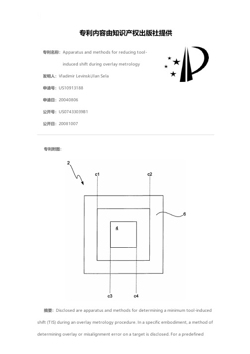
专利名称：Apparatus and methods for reducing tool-induced shift during overlay metrology发明人：Vladimir Levinski,Ilan Sela申请号：US10913188申请日：20040806公开号：US07433039B1公开日：20081007专利内容由知识产权出版社提供专利附图：摘要：Disclosed are apparatus and methods for determining a minimum tool-induced shift (TIS) during an overlay metrology procedure. In a specific embodiment, a method of determining overlay or misalignment error on a target is disclosed. For a predefinednumber of positions of a target within a field of view (FOV) of a metrology tool, the following operations are performed: (i) determining a tool-induced shift (TIS) parameter value for each predefined position of the target within the FOV based on at least one overlay measurement obtained from the target at the each position (for example, based on overlay measurements at 0 and 180 degrees of wafer orientation) and (ii) determining a minimum TIS parameter value and its corresponding FOV position from the plurality of determined TIS parameters values at the predefined positions of the target within the FOV. The FOV position that corresponds to the minimum TIS is then defined as an appropriate position for the actual overlay measurement and the value of minimum TIS is used for overlay correction.申请人：Vladimir Levinski,Ilan Sela地址：Nazareth Ilit IL,Haifa IL国籍：IL,IL代理机构：Weaver Austin Villeneuve & Sampson LLP更多信息请下载全文后查看。

专利名称：Workflow predictive analytics Engine发明人：Manuel Vegas Santiago,Travis Frosch,ElodieWeber,Eszter Csernai,ErazmusGerencser,Bence Lantos,AndrasKerekes,Andras Lanczky申请号：US16456656申请日：20190628公开号：US20200160984A1公开日：20200521专利内容由知识产权出版社提供专利附图：摘要：Systems, methods, and apparatus to generate and utilize predictive workflowanalytics and inferencing are disclosed and described. An example predictive workflow analytics apparatus includes a data store to receive healthcare workflow data including at least one of a schedule or a worklist including a patient and an activity in the at least one of the schedule or the worklist involving the patient. The example apparatus includes a data access layer to combine the healthcare workflow data with non-healthcare data to enrich the healthcare workflow data for analysis with respect to the patient. The example apparatus includes an inferencing engine to generate a prediction including a probability of patient no-show to the activity by processing the combined, enriched healthcare workflow data using a model and triggering a corrective action proportional to the probability of patient no-show.申请人：GE Precision Healthcare LLC地址：Wauwatosa WI US国籍：US更多信息请下载全文后查看。

hec-ras的thomas sorting method "HEC-RAS's Thomas Sorting Method: Unlocking the Power of River Hydraulic Modeling"Introduction:HEC-RAS (Hydrologic Engineering Centers River Analysis System) is a widely used software tool for hydraulic modeling of rivers and other water bodies. Among its numerous features, the Thomas Sorting Method provides an efficient approach for handling complex river geometries, minimizing computational effort, and optimizing simulation results. In this article, we will explore the Thomas Sorting Method in detail, step by step, to understand its significance and application.Step 1: Understanding the Basics of Hydraulic ModelingBefore delving into the intricacies of the Thomas Sorting Method, it is important to grasp the fundamentals of hydraulic modeling. Hydraulic modeling involves simulating the flow of water in rivers or channels using mathematical equations. The goal is to analyze and predict water levels, velocities, and other hydraulic parameters,which are crucial for designing and evaluating water infrastructure projects effectively.Step 2: Introduction to River GeometryThe geometry of a river is a critical component in hydraulic modeling. Rivers are often characterized by varying channel widths, slopes, bends, and obstructions such as bridges or culverts. Accurately representing these features in the computational model is essential for obtaining reliable results. However, dealing with complex geometries can be computationally intensive andtime-consuming.Step 3: Challenges Faced in Model ComputationWhen modeling complex river geometries, the standard practice is to divide the river cross-section into a series of computational cells or elements. These elements are typically triangles or rectangles, representing small sections of the overall river profile. However, during model computation, unstructured mesh configurations can lead to inefficiencies and inaccurate results.Inefficiencies arise because the model uses arbitrary connectivity patterns between the computational cells. This results in the need to solve large and sparse linear systems, which increases computation time. Inaccurate results occur due to numerical errors associated with the arbitrary connectivity between cells.Step 4: Thomas Sorting Method - Enhancing Computational EfficiencyThe Thomas Sorting Method is an innovative approach incorporated into HEC-RAS to enhance computational efficiency while maintaining accuracy. The method rearranges the computational elements based on their connectivity patterns, resulting in a highly structured mesh configuration. This structured configuration minimizes the computational effort required to solve the model equations. Consequently, it improves the overall computational efficiency and reduces model computation time significantly.Step 5: Detailed Analysis of the Thomas Sorting MethodThe Thomas Sorting Method primarily consists of three steps:Step 5.1: Identification of Critical Cross-Sections:HEC-RAS automatically identifies the critical cross-sections in the river model using an optimization algorithm. These criticalcross-sections are areas where high water velocities or steep slopes are present. By focusing computational efforts on these critical areas, the Thomas Sorting Method optimizes the accuracy of the final results.Step 5.2: Sorting of Cross-Sections:Once the critical cross-sections are identified, the Thomas Sorting Method arranges them in a certain order. This order is determined by considering the connectivity between the critical cross-sections and ensuring a structured mesh configuration.Step 5.3: Solution of Model Equations:Finally, the model equations are solved in the rearranged order of cross-sections. This structured approach simplifies the computational process, resulting in improved efficiency and accuracy compared to unstructured mesh configurations.Step 6: Benefits and Applications of the Thomas Sorting MethodThe Thomas Sorting Method offers several benefits and has diverse applications. Some key advantages include:1. Improved Computational Efficiency: The Thomas Sorting Method significantly reduces computation time by streamlining the process and reducing the complexity of solving the model equations.2. Enhanced Accuracy: The structured mesh configuration resulting from the Thomas Sorting Method minimizes numerical errors, leading to more accurate predictions of hydraulic parameters.3. Compatibility: The Thomas Sorting Method is compatible with other modules and features within HEC-RAS, facilitating seamless integration into existing hydraulic models.4. Application Flexibility: The method can be applied to various types of river systems, whether they contain simple or highly complex geometries.Conclusion:The Thomas Sorting Method in HEC-RAS revolutionizes the way hydraulic modeling is approached, providing improved computational efficiency and accuracy. By rearranging computational elements in a structured mesh configuration, the method streamlines model computation and reduces numerical errors. The Thomas Sorting Method opens new pathways for engineers and researchers to optimize their hydraulic modeling efforts, ultimately leading to better-informed decision-making in river management and infrastructure design.。

Speeded-Up Robust Features (SURF)Herbert Bay a ,Andreas Essa,*,Tinne Tuytelaars b ,Luc Van Goola,ba ETH Zurich,BIWI,Sternwartstrasse 7,CH-8092Zurich,Switzerland bK.U.Leuven,ESAT-PSI,Kasteelpark Arenberg 10,B-3001Leuven,BelgiumReceived 31October 2006;accepted 5September 2007Available online 15December 2007AbstractThis article presents a novel scale-and rotation-invariant detector and descriptor,coined SURF (Speeded-Up Robust Features).SURF approximates or even outperforms previously proposed schemes with respect to repeatability,distinctiveness,and robustness,yet can be computed and compared much faster.This is achieved by relying on integral images for image convolutions;by building on the strengths of the leading existing detectors and descriptors (specifically,using a Hessian matrix-based measure for the detector,and a distribution-based descriptor);and by sim-plifying these methods to the essential.This leads to a combination of novel detection,description,and matching steps.The paper encompasses a detailed description of the detector and descriptor and then explores the effects of the most important param-eters.We conclude the article with SURF’s application to two challenging,yet converse goals:camera calibration as a special case of image registration,and object recognition.Our experiments underline SURF’s usefulness in a broad range of topics in computer vision.Ó2007Elsevier Inc.All rights reserved.Keywords:Interest points;Local features;Feature description;Camera calibration;Object recognition1.IntroductionThe task of finding point correspondences between two images of the same scene or object is part of many com-puter vision applications.Image registration,camera cali-bration,object recognition,and image retrieval are just a few.The search for discrete image point correspondences can be divided into three main steps.First,‘interest points’are selected at distinctive locations in the image,such as cor-ners,blobs,and T-junctions.The most valuable property of an interest point detector is its repeatability.The repeat-ability expresses the reliability of a detector for finding the same physical interest points under different viewing condi-tions.Next,the neighbourhood of every interest point is represented by a feature vector.This descriptor has to be distinctive and at the same time robust to noise,detectiondisplacements and geometric and photometric deforma-tions.Finally,the descriptor vectors are matched between different images.The matching is based on a distance between the vectors,e.g.the Mahalanobis or Euclidean dis-tance.The dimension of the descriptor has a direct impact on the time this takes,and less dimensions are desirable for fast interest point matching.However,lower dimensional feature vectors are in general less distinctive than their high-dimensional counterparts.It has been our goal to develop both a detector and descriptor that,in comparison to the state-of-the-art,are fast to compute while not sacrificing performance.In order to succeed,one has to strike a balance between the above requirements like simplifying the detection scheme while keeping it accurate,and reducing the descriptor’s size while keeping it sufficiently distinctive.A wide variety of detectors and descriptors have already been proposed in the literature (e.g.[21,24,27,39,25]).Also,detailed comparisons and evaluations on benchmarking datasets have been performed [28,30,31].Our fast detector and descriptor,called SURF (Speeded-Up Robust1077-3142/$-see front matter Ó2007Elsevier Inc.All rights reserved.doi:10.1016/j.cviu.2007.09.014*Corresponding author.E-mail address:aess@vision.ee.ethz.ch (A.Ess)./locate/cviuAvailable online at Computer Vision and Image Understanding 110(2008)346–359Features),was introduced in[4].It is built on the insights gained from this previous work.In our experiments on these benchmarking datasets,SURF’s detector and descriptor are not only faster,but the former is also more repeatable and the latter more distinctive.We focus on scale and in-plane rotation-invariant detec-tors and descriptors.These seem to offer a good compromise between feature complexity and robustness to commonly occurring photometric deformations.Skew,anisotropic scaling,and perspective effects are assumed to be second order effects,that are covered to some degree by the overall robustness of the descriptor.Note that the descriptor can be extended towards affine-invariant regions using affine normalisation of the ellipse(cf.[31]),although this will have an impact on the computation time.Extending the detector, on the other hand,is less straightforward.Concerning the photometric deformations,we assume a simple linear model with a bias(offset)and contrast change(scale factor).Nei-ther detector nor descriptor use colour information.The article is structured as follows.In Section2,we give a review over previous work in interest point detection and description.In Section3,we describe the strategy applied for fast and robust interest point detection.The input image is analysed at different scales in order to guarantee invariance to scale changes.The detected interest points are provided with a rotation and scale-invariant descriptor in Section4.Furthermore,a simple and efficientfirst-line indexing technique,based on the contrast of the interest point with its surrounding,is proposed.In Section5,some of the available parameters and their effects are discussed,including the benefits of an upright version(not invariant to image rotation).We also investi-gate SURF’s performance in two important application scenarios.First,we consider a special case of image regis-tration,namely the problem of camera calibration for3D reconstruction.Second,we will explore SURF’s applica-tion to an object recognition experiment.Both applications highlight SURF’s benefits in terms of speed and robustness as opposed to other strategies.The article is concluded in Section6.2.Related work2.1.Interest point detectionThe most widely used detector is probably the Harris corner detector[15],proposed back in1988.It is based on the eigenvalues of the second moment matrix.However, Harris corners are not scale invariant.Lindeberg[21]intro-duced the concept of automatic scale selection.This allows to detect interest points in an image,each with their own characteristic scale.He experimented with both the deter-minant of the Hessian matrix as well as the Laplacian (which corresponds to the trace of the Hessian matrix)to detect blob-like structures.Mikolajczyk and Schmid[26] refined this method,creating robust and scale-invariant feature detectors with high repeatability,which they coined Harris-Laplace and Hessian-Laplace.They used a(scale-adapted)Harris measure or the determinant of the Hessian matrix to select the location,and the Laplacian to select the scale.Focusing on speed,Lowe[23]proposed to approxi-mate the Laplacian of Gaussians(LoG)by a Difference of Gaussians(DoG)filter.Several other scale-invariant interest point detectors have been proposed.Examples are the salient region detec-tor,proposed by Kadir and Brady[17],which maximises the entropy within the region,and the edge-based region detector proposed by Jurie and Schmid[16].They seem less amenable to acceleration though.Also several affine-invari-ant feature detectors have been proposed that can cope with wider viewpoint changes.However,these fall outside the scope of this article.From studying the existing detectors and from published comparisons[29,30],we can conclude that Hessian-based detectors are more stable and repeatable than their Harris-based counterparts.Moreover,using the determinant of the Hessian matrix rather than its trace(the Laplacian) seems advantageous,as itfires less on elongated,ill-localised structures.We also observed that approximations like the DoG can bring speed at a low cost in terms of lost accuracy.2.2.Interest point descriptionAn even larger variety of feature descriptors has been proposed,like Gaussian derivatives[11],moment invari-ants[32],complex features[1],steerablefilters[12], phase-based local features[6],and descriptors representing the distribution of smaller-scale features within the interest point neighbourhood.The latter,introduced by Lowe[24], have been shown to outperform the others[28].This can be explained by the fact that they capture a substantial amount of information about the spatial intensity patterns, while at the same time being robust to small deformations or localisation errors.The descriptor in[24],called SIFT for short,computes a histogram of local oriented gradients around the interest point and stores the bins in a128D vec-tor(8orientation bins for each of4Â4location bins).Various refinements on this basic scheme have been pro-posed.Ke and Sukthankar[18]applied PCA on the gradi-ent image around the detected interest point.This PCA-SIFT yields a36D descriptor which is fast for matching, but proved to be less distinctive than SIFT in a second comparative study by Mikolajczyk and Schmid[30];and applying PCA slows down feature computation.In the same paper[30],the authors proposed a variant of SIFT, called GLOH,which proved to be even more distinctive with the same number of dimensions.However,GLOH is computationally more expensive as it uses again PCA for data compression.The SIFT descriptor still seems the most appealing descriptor for practical uses,and hence also the most widely used nowadays.It is distinctive and relatively fast, which is crucial for on-line applications.Recently,Se et al.[37]implemented SIFT on a Field ProgrammableH.Bay et al./Computer Vision and Image Understanding110(2008)346–359347Gate Array(FPGA)and improved its speed by an order of magnitude.Meanwhile,Grabner et al.[14]also used inte-gral images to approximate SIFT.Their detection step is based on difference-of-mean(without interpolation),their description step on integral histograms.They achieve about the same speed as we do(though the description step is constant in speed),but at the cost of reduced quality compared to SIFT.Generally,the high dimensionality of the descriptor is a drawback of SIFT at the matching step. For on-line applications relying only on a regular PC,each one of the three steps(detection,description,matching)has to be fast.An entire body of work is available on speeding up the matching step.All of them come at the expense of getting an approximative matching.Methods include the best-bin-first proposed by Lowe[24],balltrees[35],vocabulary trees[34],locality sensitive hashing[9],or redundant bit vectors[13].Complementary to this,we suggest the use of the Hessian matrix’s trace to significantly increase the matching speed.Together with the descriptor’s low dimen-sionality,any matching algorithm is bound to perform faster.3.Interest point detectionOur approach for interest point detection uses a very basic Hessian matrix approximation.This lends itself to the use of integral images as made popular by Viola and Jones[41],which reduces the computation time drastically. Integral imagesfit in the more general framework of box-lets,as proposed by Simard et al.[38].3.1.Integral imagesIn order to make the article more self-contained,we briefly discuss the concept of integral images.They allow for fast computation of box type convolutionfilters.The entry of an integral image I RðxÞat a location x¼ðx;yÞT represents the sum of all pixels in the input image I within a rectangular region formed by the origin and x.I RðxÞ¼X i6xi¼0X j6yj¼0Iði;jÞð1ÞOnce the integral image has been computed,it takes three additions to calculate the sum of the intensities over any upright,rectangular area(see Fig.1).Hence,the calcu-lation time is independent of its size.This is important in our approach,as we use bigfilter sizes.3.2.Hessian matrix-based interest pointsWe base our detector on the Hessian matrix because of its good performance in accuracy.More precisely,we detect blob-like structures at locations where the determi-nant is maximum.In contrast to the Hessian-Laplace detector by Mikolajczyk and Schmid[26],we rely on the determinant of the Hessian also for the scale selection,as done by Lindeberg[21].Given a point x¼ðx;yÞin an image I,the Hessian matrix Hðx;rÞin x at scale r is defined as followsHðx;rÞ¼L xxðx;rÞL xyðx;rÞL xyðx;rÞL yyðx;rÞ;ð2Þwhere L xxðx;rÞis the convolution of the Gaussian secondorder derivative o22gðrÞwith the image I in point x,and similarly for L xyðx;rÞand L yyðx;rÞ.Gaussians are optimal for scale-space analysis[19,20], but in practice they have to be discretised and cropped (Fig.2,left half).This leads to a loss in repeatability under image rotations around odd multiples of p.This weakness holds for Hessian-based detectors in general. Fig.3shows the repeatability rate of two detectors based on the Hessian matrix for pure image rotation. The repeatability attains a maximum around multiples of p2.This is due to the square shape of thefilter.Nev-ertheless,the detectors still perform well,and the slight decrease in performance does not outweigh the advan-tage of fast convolutions brought by the discretisation and cropping.As realfilters are non-ideal in any case, and given Lowe’s success with his LoG approximations, we push the approximation for the Hessian matrix even further with boxfilters(in the right half of Fig.2). These approximate second order Gaussian derivatives and can be evaluated at a very low computationalcost ing integral images,it takes only three additions and four memory accesses to calculate the sum of intensities inside a rectangular region of anysize.Fig.2.Left to right:The(discretised and cropped)Gaussian second order partial derivative in y-(L yy)and xy-direction(L xy),respectively;our approximation for the second order Gaussian partial derivative in y-(D yy) and xy-direction(D xy).The grey regions are equal to zero.348H.Bay et al./Computer Vision and Image Understanding110(2008)346–359using integral images.The calculation time therefore is independent of thefilter size.As shown in Section5 and Fig.3,the performance is comparable or better than with the discretised and cropped Gaussians.The9Â9boxfilters in Fig.2are approximations of a Gaussian with r¼1:2and represent the lowest scale(i.e. highest spatial resolution)for computing the blob response maps.We will denote them by D xx,D yy,and D xy.The weights applied to the rectangular regions are kept simple for computational efficiency.This yieldsdetðH approxÞ¼D xx D yyÀðwD xyÞ2:ð3ÞThe relative weight w of thefilter responses is used to bal-ance the expression for the Hessian’s determinant.This is needed for the energy conservation between the Gaussian kernels and the approximated Gaussian kernels,w¼j L xyð1:2ÞjFj D yyð9ÞjFj L yyð1:2ÞjFj D xyð9ÞjF¼0:912:::’0:9;ð4Þwhere j x jF is the Frobenius norm.Notice that for theoret-ical correctness,the weighting changes depending on the scale.In practice,we keep this factor constant,as this did not have a significant impact on the results in our experiments.Furthermore,thefilter responses are normalised with respect to their size.This guarantees a constant Frobenius norm for anyfilter size,an important aspect for the scale space analysis as discussed in the next section.The approximated determinant of the Hessian repre-sents the blob response in the image at location x.These responses are stored in a blob response map over different scales,and local maxima are detected as explained in Sec-tion3.4.3.3.Scale space representationInterest points need to be found at different scales,not least because the search of correspondences often requires their comparison in images where they are seen at different scales.Scale spaces are usually implemented as an image pyramid.The images are repeatedly smoothed with a Gaussian and then sub-sampled in order to achieve a higher level of the pyramid.Lowe[24]subtracts these pyr-amid layers in order to get the DoG(Difference of Gaussi-ans)images where edges and blobs can be found.Due to the use of boxfilters and integral images,we do not have to iteratively apply the samefilter to the output of a previouslyfiltered layer,but instead can apply boxfilters of any size at exactly the same speed directly on the original image and even in parallel(although the latter is not exploited here).Therefore,the scale space is analysed by up-scaling thefilter size rather than iteratively reducing the image size,Fig.4.The output of the9Â9filter,intro-duced in previous section,is considered as the initial scale layer,to which we will refer as scale s¼1:2(approximating Gaussian derivatives with r¼1:2).The following layers are obtained byfiltering the image with gradually bigger masks,taking into account the discrete nature of integral images and the specific structure of ourfilters.Note that our main motivation for this type of sampling is its computational efficiency.Furthermore,as we do not have to downsample the image,there is no aliasing.On the downside,boxfilters preserve high-frequency compo-nents that can get lost in zoomed-out variants of the same scene,which can limit scale-invariance.This was however not noticeable in our experiments.The scale space is divided into octaves.An octave repre-sents a series offilter response maps obtained by convolv-ing the same input image with afilter of increasing size.In total,an octave encompasses a scaling factor of2(which implies that one needs to more than double thefilter size, see below).Each octave is subdivided into a constant num-ber of scale levels.Due to the discrete nature of integral images,the minimum scale difference between two subse-quent scales depends on the length l0of the positive or neg-ative lobes of the partial second order derivative in the direction of derivation(x or y),which is set to a third of thefilter size length.For the9Â9filter,this length l0is 3.For two successive levels,we must increase this size byFig.3.Top:Repeatability score for image rotation of up to180°.Hessian-based detectors have in general a lower repeatability score for anglesFig.4.Instead of iteratively reducing the image size(left),the use ofintegral images allows the up-scaling of thefilter at constant cost(right).H.Bay et al./Computer Vision and Image Understanding110(2008)346–359349a minimum of 2pixels (1pixel on every side)in order to keep the size uneven and thus ensure the presence of the central pixel.This results in a total increase of the mask size by 6pixels (see Fig.5).Note that for dimensions different from l 0(e.g.the width of the central band for the vertical filter in Fig.5),rescaling the mask introduces rounding-offerrors.However,since these errors are typically much smaller than l 0,this is an acceptable approximation.The construction of the scale space starts with the 9Â9filter,which calculates the blob response of the image for the smallest scale.Then,filters with sizes 15Â15,21Â21,and 27Â27are applied,by which even more than a scale change of two has been achieved.But this is needed,as a 3D non-maximum suppression is applied both spa-tially and over the neighbouring scales.Hence,the first and last Hessian response maps in the stack cannot contain such maxima themselves,as they are used for reasons of comparison only.Therefore,after interpolation,see Sec-tion 3.4,the smallest possible scale is r ¼1:6¼1:2129corre-sponding to a filter size of 12Â12,and the highest to r ¼3:2¼1:224.For more details,we refer to [2].Similar considerations hold for the other octaves.For each new octave,the filter size increase is doubled (going from 6–12to 24–48).At the same time,the sampling inter-vals for the extraction of the interest points can be doubled as well for every new octave.This reduces the computation time and the loss in accuracy is comparable to the image sub-sampling of the traditional approaches.The filter sizes for the second octave are 15,27,39,51.A third octave is com-puted with the filter sizes 27,51,75,99and,if the original image size is still larger than the corresponding filter sizes,the scale space analysis is performed for a fourth octave,using the filter sizes 51,99,147,and 195.Fig.6gives an over-view of the filter sizes for the first three octaves.Further octaves can be computed in a similar way.In typical scale-space analysis however,the number of detected interest points per octave decays very quickly,cf.Fig.7.The large scale changes,especially between the first fil-ters within these octaves (from 9to 15is a change of 1.7),renders the sampling of scales quite crude.Therefore,we have also implemented a scale space with a finer sam-pling of the scales.This computes the integral image on the image up-scaled by a factor of 2,and then starts the first octave by filtering with a filter of size 15.Additional filter sizes are 21,27,33,and 39.Then a second octave starts,again using filters which now increase their sizes by 12pixels,after which a third and fourth octave follow.Now the scale change between the first two filters is only 1.4(21/15).The lowest scale for the accurate version that can be detected through quadratic interpolation is s ¼ð1:2189Þ=2¼1:2.As the Frobenius norm remains constant for our filters at any size,they are already scale normalised,and no fur-ther weighting of the filter response is required,for more information on that topic,see [22].3.4.Interest point localisationIn order to localise interest points in the image and over scales,a non-maximum suppression in a 3Â3Â3neigh-bourhood is applied.Specifically,we use a fast variant introduced by Neubeck and Van Gool [33].The maxima of the determinant of the Hessian matrix are then interpo-lated in scale and image space with the method proposed by Brown and Lowe [5].Scale space interpolation is especially important in our case,as the difference in scale between the first layers of every octave is relatively large.Fig.8shows an example of the detected interest points using our ‘Fast-Hessian’detector.4.Interest point description and matchingOur descriptor describes the distribution of the intensity content within the interest point neighbourhood,similartoFig.5.Filters D yy (top)and D xy (bottom)for two successive scale levels (9Â9and 15Â15).The length of the dark lobe can only be increased by an even number of pixels in order to guarantee the presence of a central pixel(top).Fig.6.Graphical representation of the filter side lengths for three different octaves.The logarithmic horizontal axis represents the scales.Note that the octaves are overlapping in order to cover all possible scales seamlessly.350H.Bay et al./Computer Vision and Image Understanding 110(2008)346–359the gradient information extracted by SIFT [24]and its variants.We build on the distribution of first order Haar wavelet responses in x and y direction rather than the gra-dient,exploit integral images for speed,and use only 64D.This reduces the time for feature computation and match-ing,and has proven to simultaneously increase the robust-ness.Furthermore,we present a new indexing step based on the sign of the Laplacian,which increases not only the robustness of the descriptor,but also the matching speed (by a factor of 2in the best case).We refer to our detec-tor-descriptor scheme as SURF—Speeded-Up Robust Features.The first step consists of fixing a reproducible orienta-tion based on information from a circular region around the interest point.Then,we construct a square region aligned to the selected orientation and extract the SURF descriptor from it.Finally,features are matched between two images.These three steps are explained in the following.4.1.Orientation assignmentIn order to be invariant to image rotation,we identify a reproducible orientation for the interest points.For that purpose,we first calculate the Haar wavelet responses in x and y direction within a circular neighbourhood of radius 6s around the interest point,with s the scale at which the interest point was detected.The sampling step is scale dependent and chosen to be s .In keeping with the rest,also the size of the wavelets are scale dependent and set to a side length of 4s .Therefore,we can again use integral images for fast filtering.The used filters are shown in Fig.9.Only six operations are needed to compute the response in x or y direction at any scale.Once the wavelet responses are calculated and weighted with a Gaussian (r ¼2s )centred at the interest point,the responses are represented as points in a space with the hor-izontal response strength along the abscissa and the vertical response strength along the ordinate.The dominant orien-tation is estimated by calculating the sum of all responses within a sliding orientation window of size p ,see Fig.10.The horizontal and vertical responses within the window are summed.The two summed responses then yield a local orientation vector.The longest such vector over all win-dows defines the orientation of the interest point.The size of the sliding window is a parameter which had to be cho-sen carefully.Small sizes fire on single dominating gradi-ents,large sizes tend to yield maxima in vector length that are not outspoken.Both result in a misorientation of the interest point.Note that for many applications,rotation invariance is not necessary.Experiments of using the upright version of SURF (U-SURF,for short)for object detection can be found in [3,4].U-SURF is faster to compute and can increase distinctivity,while maintaining a robustness to rotation of about ±15°.4.2.Descriptor based on sum of Haar wavelet responses For the extraction of the descriptor,the first step con-sists of constructing a square region centred around the interest point and oriented along the orientation selected in previous section.The size of this window is 20s .Exam-ples of such square regions are illustrated in Fig.11.The region is split up regularly into smaller 4Â4square sub-regions.This preserves important spatial information.For each sub-region,we compute Haar waveletresponsesFig.8.Detected interest points for a Sunflower field.This kind of scenes shows the nature of the features obtained using Hessian-baseddetectors.Fig.9.Haar wavelet filters to compute the responses in x (left)and y direction (right).The dark parts have the weight À1and the light parts þ1.H.Bay et al./Computer Vision and Image Understanding 110(2008)346–359351at 5Â5regularly spaced sample points.For reasons of simplicity,we call d x the Haar wavelet response in horizon-tal direction and d y the Haar wavelet response in vertical direction (filter size 2s ),see Fig.9again.‘‘Horizontal’’and ‘‘vertical’’here is defined in relation to the selected interest point orientation (see Fig.12).1To increase the robustness towards geometric deformations and localisa-tion errors,the responses d x and d y are first weighted with a Gaussian (r ¼3:3s )centred at the interest point.Then,the wavelet responses d x and d y are summed up over each sub-region and form a first set of entries in thefeature vector.In order to bring in information about the polarity of the intensity changes,we also extract the sum of the absolute values of the responses,j d x j and j d y j .Hence,each sub-region has a 4D descriptor vector v for its underlying intensity structure v ¼ðP d x ;P d y ;Pj d x j ;P j d y jÞ.Concatenating this for all 4Â4sub-regions,this results in a descriptor vector of length 64.The wavelet responses are invariant to a bias in illumina-tion (offset).Invariance to contrast (a scale factor)is achieved by turning the descriptor into a unit vector.Fig.13shows the properties of the descriptor for three distinctively different image-intensity patterns within a sub-region.One can imagine combinations of such local intensity patterns,resulting in a distinctive descriptor.SURF is,up to some point,similar in concept as SIFT,in that they both focus on the spatial distribution of gradi-ent information.Nevertheless,SURF outperforms SIFT in practically all cases,as shown in Section 5.We believe this is due to the fact that SURF integrates the gradient infor-mation within a subpatch,whereas SIFT depends on the orientations of the individual gradients.This makesSURFFig.10.Orientation assignment:a sliding orientation window of size p3detects the dominant orientation of the Gaussian weighted Haar wavelet responses at every sample pointwithin a circular neighbourhood around the interest point.Fig.11.Detail of the Graffiti scene showing thesize of the oriented descriptor window at different scales.Fig.12.To build the descriptor,an oriented quadratic grid with 4Â4square sub-regions is laid over the interest point (left).For each square,the wavelet responses are computed from 5Â5samples (for illustrative purposes,we show only 2Â2sub-divisions here).For each field,we collect the sums d x ,j d x j ;d y ,and j d y j ,computed relatively to the orientation of the grid (right).1For efficiency reasons,the Haar wavelets are calculated in the unrotated image and the responses arethen interpolated,instead of actually rotating the image.Fig.13.The descriptor entries of a sub-region represent the nature of the underlying intensity pattern.Left:In case of a homogeneous region,all values are relatively low.Middle:In presence of frequencies in x direction,the value of P j d x j is high,but all others remain low.Ifthe intensity is gradually increasing in x direction,both values P d x andP j d x j are high.352H.Bay et al./Computer Vision and Image Understanding 110(2008)346–359。

See discussions, stats, and author profiles for this publication at: /publication/225138825Two-Frame Motion Estimation Based on Polynomial ExpansionCHAPTER · DECEMBER 2002DOI: 10.1007/3-540-45103-X_50 · Source: DBLP CITATIONS 57READS1581 AUTHOR:Gunnar FarnebäckContextVision29 PUBLICATIONS 750 CITATIONSSEE PROFILEAvailable from: Gunnar FarnebäckRetrieved on: 17 November 2015//the OpenCV source code locate %OPENCV%\sources\modules\video\src\optflowgf.cpp 函数calcOpticalFlowFarneback （）计算稠密光流Two-Frame Motion Estimation Based onPolynomial ExpansionGunnar Farneb¨a ckComputer Vision Laboratory,Link¨o ping University,SE-58183Link¨o ping,Swedengf@isy.liu.sehttp://www.isy.liu.se/cvl/Abstract.This paper presents a novel two-frame motion estimation al-gorithm.Thefirst step is to approximate each neighborhood of bothframes by quadratic polynomials,which can be done efficiently using thepolynomial expansion transform.From observing how an exact polyno-mial transforms under translation a method to estimate displacementfields from the polynomial expansion coefficients is derived and aftera series of refinements leads to a robust algorithm.Evaluation on theYosemite sequence shows good results.1IntroductionIn previous work we have developed orientation tensor based algorithms to es-timate motion,with excellent results both with respect to accuracy and speed [1,2].A limitation of those,however,is that the estimation of the spatiotem-poral orientation tensors requires the motionfield to be temporally consistent. This is often the case but turned out to be a problem in the WITAS project [3],where image sequences are obtained by a helicopter-mounted camera.Due to high frequency vibrations from the helicopter affecting the camera system, there are large,quickly varying,and difficult to predict displacements between successive frames.A natural solution is to estimate the motion,or displacement,field from only two frames and try to compensate for the background motion.This paper presents a novel method to estimate displacement.It is related to our orienta-tion tensor methods in that thefirst processing step,a signal transform called polynomial expansion,is common.Naturally this is only done spatially now,in-stead of spatiotemporally.Another common theme is the inclusion of parametric motion models in the algorithms.2Polynomial ExpansionThe idea of polynomial expansion is to approximate some neighborhood of each pixel with a polynomial.Here we are only interested in quadratic polynomials, giving us the local signal model,expressed in a local coordinate system,f(x)∼x T Ax+b T x+c,(1)where A is a symmetric matrix,b a vector and c a scalar.The coefficients are estimated from a weighted least squaresfit to the signal values in the neigh-borhood.The weighting has two components called certainty and applicability. These terms are the same as in normalized convolution[4–6],which polyno-mial expansion is based on.The certainty is coupled to the signal values in the neighborhood.For example it is generally a good idea to set the certainty to zero outside the image.Then neighborhood points outside the image have no impact on the coefficient estimation.The applicability determines the relative weight of points in the neighborhood based on their position in the neighbor-hood.Typically one wants to give most weight to the center point and let the weights decrease radially.The width of the applicability determines the scale of the structures which will be captured by the expansion coefficients.While this may sound computationally very demanding it turns out that it can be implemented efficiently by a hierarchical scheme of separable convolu-tions.Further details on this can be found in[6].3Displacement EstimationSince the result of polynomial expansion is that each neighborhood is approx-imated by a polynomial,we start by analyzing what happens if a polynomial undergoes an ideal translation.Consider the exact quadratic polynomialf1(x)=x T A1x+b T1x+c1(2) and construct a new signal f2by a global displacement by d,f2(x)=f1(x−d)=(x−d)T A1(x−d)+b T1(x−d)+c1=x T A1x+(b1−2A1d)T x+d T A1d−b T1d+c1=x T A2x+b T2x+c2.(3) Equating the coefficients in the quadratic polynomials yieldsA2=A1,(4)b2=b1−2A1d,(5)c2=d T A1d−b T1d+c1.(6) The key observation is that by equation(5)we can solve for the translation d, at least if A1is non-singular,2A1d=−(b2−b1),(7)d=−12A−11(b2−b1).(8)We note that this observation holds for any signal dimensionality.3.1Practical ConsiderationsObviously the assumptions about an entire signal being a single polynomial and a global translation relating the two signals are quite unrealistic.Still the basic relation(7)can be used for real signals,although errors are introduced when the assumptions are relaxed.The question is whether these errors can be kept small enough to give a useful algorithm.To begin with we replace the global polynomial in equation(2)with local polynomial approximations.Thus we start by doing a polynomial expansion of both images,giving us expansion coefficients A1(x),b1(x),and c1(x)for the first image and A2(x),b2(x),and c2(x)for the second image.Ideally this should give A1=A2according to equation(4)but in practice we have to settle for theapproximationA(x)=A1(x)+A2(x)2.(9)We also introduce∆b(x)=−12(b2(x)−b1(x))(10)to obtain the primary constraintA(x)d(x)=∆b(x),(11) where d(x)indicates that we have also replaced the global displacement in equa-tion(3)with a spatially varying displacementfield.3.2Estimation Over a NeighborhoodIn principle equation(11)can be solved pointwise,but the results turn out to be too noisy.Instead we make the assumption that the displacementfield is only slowly varying,so that we can integrate information over a neighborhood of each pixel.Thus we try tofind d(x)satisfying(11)as well as possible over a neighborhood I of x,or more formally minimizing∆x∈Iw(∆x) A(x+∆x)d(x)−∆b(x+∆x) 2,(12)where we let w(∆x)be a weight function for the points in the neighborhood. The minimum is obtained ford(x)=w A T A−1w A T∆b,(13)where we have dropped some indexing to make the expression more readable. The minimum value is given bye(x)=w∆b T∆b−d(x)Tw A T∆b.(14)In practical terms this means that we compute A T A,A T∆b,and∆b T∆b pointwise and average these with w before we solve for the displacement.Theminimum value e (x )can be used as a reversed confidence value,with small numbers indicating high confidence.The solution given by (13)exists and is unique unless the whole neighborhood is exposed to the aperture problem.Sometimes it is useful to add a certainty weight c (x +∆x )to (12).This is most easily handled by scaling A and ∆b accordingly.3.3Parameterized Displacement FieldsWe can improve robustness if the displacement field can be parameterized ac-cording to some motion model.This is straightforward for motion models which are linear in their parameters,like the affine motion model or the eight parameter model.We derive this for the eight parameter model in 2D,d x (x,y )=a 1+a 2x +a 3y +a 7x 2+a 8xy,d y (x,y )=a 4+a 5x +a 6y +a 7xy +a 8y 2.(15)We can rewrite this asd =Sp ,(16)S = 1x y 000x 2xy 0001x y xy y 2,(17)p = a 1a 2a 3a 4a 5a 6a 7a 8 T .(18)Inserting into (12)we obtain the weighted least squares problemi w i A i S i p −∆b i 2,(19)where we use i to index the coordinates in a neighborhood.The solution isp = i w i S T i A T i A i S i −1 iw i S T i A T i ∆b i .(20)We notice that like before we can compute S T A T AS and S T A T ∆b pointwise and then average these with w .Naturally (20)reduces to (13)for the constant motion model.3.4Incorporating A Priori KnowledgeA principal problem with the method so far is that we assume that the local polynomials at the same coordinates in the two signals are identical except for a displacement.Since the polynomial expansions are local models these will vary spatially,introducing errors in the constraints (11).For small displacements this is not too serious,but with larger displacements the problem increases.Fortu-nately we are not restricted to comparing two polynomials at the same coordi-nate.If we have a priori knowledge about the displacement field,we can comparethe polynomial at x in thefirst signal to the polynomial at x+˜d(x)in the second signal,where˜d(x)is the a priori displacementfield rounded to integer values. Then we effectively only need to estimate the relative displacement between the real value and the rounded a priori estimate,which hopefully is smaller.This observation is included in the algorithm by replacing equations(9)and (10)byA(x)=A1(x)+A2(˜x)2,(21)∆b(x)=−12(b2(˜x)−b1(x))+A(x)˜d(x),(22)where˜x=x+˜d(x).(23) Thefirst two terms in∆b are involved in computing the remaining displacement while the last term adds back the rounded a priori displacement.We can see that for˜d identically zero,these equations revert to(9)and(10),as would be expected.3.5Iterative and Multi-scale Displacement EstimationA consequence of the inclusion of an a priori displacementfield in the algorithm is that we can close the loop and iterate.A better a priori estimate means a smaller relative displacement,which in turn improves the chances for a good displacement estimate.We consider two different approaches,iterative displace-ment estimation and multi-scale displacement estimation.In both the approaches we iterate with the estimated displacements from one step used as a priori displacement in the next step.The a priori displacement field in thefirst step would usually be set to zero,unless actual knowledge about it is available.In thefirst approach the same polynomial expansion coefficients are used in all iterations and need only be computed once.The weak spot of this approach is in thefirst iteration.If the displacements(relative the a priori displacements) are too large,the output displacements cannot be expected to be improvements and iterating will be meaningless.The problem of too large displacements can be reduced by doing the analysis at a coarser scale.This means that we use a larger applicability for the poly-nomial expansion and/or lowpassfilter the signalfirst.The effect is that the estimation algorithm can handle larger displacements but at the same time the accuracy decreases.This observation points to the second approach with multiple scales.Start at a coarse scale to get a rough but reasonable displacement estimate and prop-agate this throughfiner scales to obtain increasingly more accurate estimates.A drawback is that we need to recompute the polynomial expansion coefficients for each scale,but this cost can be reduced by subsampling between scales.4Experimental ResultsThe algorithm has been implemented in Matlab,with certain parts in the form of C mexfiles.Source code for the implementation is available fromhttp://www.isy.liu.se/~gf.The algorithm has been evaluated on a commonly used test sequence with known velocityfield,Lynn Quam’s Yosemite sequence[7],figure1.This synthetic sequence was generated with the help of a digital terrain map and therefore has a motionfield with depth variation and discontinuities at occlusion boundaries.The accuracy of the velocity estimates has been measured using the average spatiotemporal angular error,arccos(ˆv T estˆv true)[8].The sky region is excluded from the error analysis because the variations in the cloud textures induce an imageflow that is quite different from the ground truth values computed solely from the camera motion.We have estimated the displacement from the center frame and the frame before.The averaging over neighborhoods is done using a39×39Gaussian weighting function(w in equation(19))with standard deviation6.The poly-nomial expansion is done with an11×11Gaussian applicability with standard deviation1.5.In order to reduce the errors near the borders,the polynomial expansions have been computed with certainty set to zero offthe border.Addi-tionally pixels close to the borders have been given a reduced weight(see section 3.2)because the expansion coefficients still can be assumed to be less reliable there.The constant and affine motion models have been used with a single iter-ation and with three iterations at the same scale.The results and a comparison with other methods can be found in table1. Clearly this algorithm cannot compete with the most accurate ones,but that is to be expected since those take advantage of the spatio-temporal consistency over several frames.Still these results are good for a two-frame algorithm.A more thorough evaluation of the algorithm can be found in[6].The main weakness of the algorithm is the assumption of a slowly varying displacementfield,causing discontinuities to be smoothed out.This can be solved by combining the algorithm with a simultaneous segmentation procedure,e.g. the one used in[2].AcknowledgementsThe work presented in this paper was supported by WITAS,the Wallenberg lab-oratory on Information Technology and Autonomous Systems,which is gratefully acknowledged.References1.Farneb¨a ck,G.:Fast and Accurate Motion Estimation using Orientation Tensorsand Parametric Motion Models.In:Proceedings of15th International Conference on Pattern Recognition.Volume1.,Barcelona,Spain,IAPR(2000)135–139Fig.1.One frame of the Yosemite sequence(subsampled).parison with other methods,Yosemite sequence.The sky region is ex-cluded for all results.Technique Average Standard Densityerror deviationLucas&Kanade[9] 2.80◦3.82◦35%Uras et al.[10] 3.37◦3.37◦14.7%Fleet&Jepson[11] 2.97◦5.76◦34.1%Black&Anandan[12] 4.46◦4.21◦100%Szeliski&Coughlan[13] 2.45◦3.05◦100%Black&Jepson[14] 2.29◦2.25◦100%Ju et al.[15] 2.16◦2.0◦100%Karlholm[16] 2.06◦1.72◦100%Lai&Vemuri[17] 1.99◦1.41◦100%Bab-Hadiashar&Suter[18] 1.97◦1.96◦100%M´e min&P´e rez[19] 1.58◦1.21◦100%Farneb¨a ck,constant motion[1,6] 1.94◦2.31◦100%Farneb¨a ck,affine motion[1,6] 1.40◦2.57◦100%Farneb¨a ck,segmentation[2,6] 1.14◦2.14◦100%Constant motion,1iteration 3.94◦4.23◦100%Constant motion,3iterations 2.60◦2.27◦100%Affine motion,1iteration 4.19◦6.76◦100%Affine motion,3iterations 2.08◦2.45◦100%2.Farneb¨a ck,G.:Very High Accuracy Velocity Estimation using Orientation Ten-sors,Parametric Motion,and Simultaneous Segmentation of the Motion Field.In: Proceedings of the Eighth IEEE International Conference on Computer Vision.Volume I.,Vancouver,Canada(2001)171–1773.URL:http://www.ida.liu.se/ext/witas/.4.Knutsson,H.,Westin,C.F.:Normalized and Differential Convolution:Methods forInterpolation and Filtering of Incomplete and Uncertain Data.In:Proceedings of IEEE Computer Society Conference on Computer Vision and Pattern Recognition, New York City,USA,IEEE(1993)515–5235.Westin,C.F.:A Tensor Framework for Multidimensional Signal Processing.PhDthesis,Link¨o ping University,Sweden,SE-58183Link¨o ping,Sweden(1994)Disser-tation No348,ISBN91-7871-421-4.6.Farneb¨a ck,G.:Polynomial Expansion for Orientation and Motion Estimation.PhD thesis,Link¨o ping University,Sweden,SE-58183Link¨o ping,Sweden(2002) Dissertation No790,ISBN91-7373-475-6.7.Heeger,D.J.:Model for the extraction of imageflow.J.Opt.Soc.Am.A4(1987)1455–14718.Barron,J.L.,Fleet,D.J.,Beauchemin,S.S.:Performance of opticalflow techniques.Int.J.of Computer Vision12(1994)43–779.Lucas,B.,Kanade,T.:An Iterative Image Registration Technique with Applica-tions to Stereo Vision.In:Proc.Darpa IU Workshop.(1981)121–13010.Uras,S.,Girosi,F.,Verri,A.,Torre,V.:A computational approach to motionperception.Biological Cybernetics(1988)79–9711.Fleet,D.J.,Jepson,A.D.:Computation of Component Image Velocity from LocalPhase Information.Int.Journal of Computer Vision5(1990)77–10412.Black,M.J.,Anandan,P.:The robust estimation of multiple motions:Parametricand piecewise-smoothflowfiputer Vision and Image Understanding63 (1996)75–10413.Szeliski,R.,Coughlan,J.:Hierarchical spline-based image registration.In:Proc.IEEE Conference on Computer Vision Pattern Recognition,Seattle,Washington (1994)194–20114.Black,M.J.,Jepson, A.:Estimating opticalflow in segmented images usingvariable-order parametric models with local deformations.IEEE Transactions on Pattern Analysis and Machine Intelligence18(1996)972–98615.Ju,S.X.,Black,M.J.,Jepson,A.D.:Skin and bones:Multi-layer,locally affine,opticalflow and regularization with transparency.In:Proceedings CVPR’96,IEEE (1996)307–31416.Karlholm,J.:Local Signal Models for Image Sequence Analysis.PhD thesis,Link¨o ping University,Sweden,SE-58183Link¨o ping,Sweden(1998)Dissertation No536,ISBN91-7219-220-8.i,S.H.,Vemuri,B.C.:Reliable and efficient computation of opticalflow.Inter-national Journal of Computer Vision29(1998)87–10518.Bab-Hadiashar,A.,Suter,D.:Robust opticflow computation.International Jour-nal of Computer Vision29(1998)59–7719.M´e min,E.,P´e rez,P.:Hierarchical estimation and segmentation of dense motionfields.International Journal of Computer Vision46(2002)129–155。