复旦大学微观经济学讲义优化

微观经济学讲义第一章导论教学目的和要求：理解经济学的定义和经济思维，掌握经济学的内容和方法，了解经济学的现实意义。

关键概念：经济学，理性行为假定，稀缺性规律，生产可能性边界，资源配置，机会成本，实证分析，规范分析，边际分析本章计划讲授4学时。

第一节经济学是什么一、经济学的定位1. 经济学是一门古老而又年轻的学科。

古老：2000年前，古希腊和古罗马时期，就产生了丰富的经济思想和出现了经济学的萌芽。

年轻：按照学术界公认的说法，经济学真正成为一门学科是以两百多年前英国经济学家亚当·斯密（Adam Smith）发表《国富论》为标志的。

2. 经济学定位于社会科学英国经济学家A·马歇尔（A · Marshall）把经济学定义为“关于人类一般生活事务的学问”。

二、理性行为假定亚当·斯密在《国富论》中所讲的“经济人假设”。

按照斯密的分析，理性的人，一般都是自私自利的，他们从自己的角度出发追求自身利益最大化。

三、稀缺性规律1. 一方面是人类需要的无限性。

2. 另一方面却是资源的有限性。

四、经济学的制度前提第一，维护人权。

第二，保护产权。

第三，理性政府。

第二节经济学的基本问题一、资源配置资源配置解决以下三大基本经济问题：1．生产什么？2．如何生产？3．为谁生产？二、资源利用资源利用问题就是要解决好如下三大基本经济问题：1．社会的生产能力为什么有时会倒退？2．如何才能不断地扩张社会的生产能力？3．谁来协调全社会的生产的稳定和发展？三、微观经济学与宏观经济学经济学按其研究的内容，可以分为微观经济学和宏观经济学。

微观经济学强调的是资源的配置，而宏观经济学强调的是资源的利用。

第三节经济学的研究方法一、实证分析与规范分析1.什么是实证分析？实证分析企图超脱或者排斥一切的价值判断，只考虑建立经济事物之间的关系，并在这些规律的作用下，分析和预测人们经济行为的结果。

简单地说，实证分析要回答的是“是什么”的问题。

高校教师微观经济学课程教学的建议一、导论二、高校教师微观经济学课程的重要性三、高校教师微观经济学课程教学建议1.注重案例分析2.灵活运用互动教学模式3.利用科技手段丰富教学内容4.根据学生需求调整教学方法5.强化评价机制四、案例分析1.北京大学教师刘明教授微观经济学课程的教学方法分析2.浙江大学教师李华老师利用案例教学的效果分析3.复旦大学教师王红教授的互动教学实践4.华东师范大学教师张丽丽的科技手段应用和丰富课程内容5.上海财经大学教师赵明的评价机制构建与优化五、结论导论高校教师微观经济学课程的教学是实现高等经济教育目标的重要环节，也是提高学生经济学专业素养的关键。

在新时代，高校教师要积极拥抱数字化和信息化时代，探索新的教学模式方法，延续和丰富教育教学改革成果，进一步凸显高校教育的品质和水准。

高校教师微观经济学课程的重要性高校教师微观经济学课程是培养学生经济学素质的重要途径，其知识体系对于建设具有国际竞争力的高素质人才、为中国实现高质量发展提供智力支持起到了重要作用。

微观经济学正是为实现完善的社会主义市场经济体制服务的学科，高校教师在这方面的任务十分重要。

高校教师微观经济学课程教学建议注重案例分析在微观经济学课程中，教师可以通过分析实际案例，让学生更加深入地理解和理解学术知识，有效的将学术理论和实践相结合，增强学生对现实经济问题分析与解决问题的能力。

灵活运用互动教学模式在教学中，教师可以灵活运用互动教学模式，让学生充分参与其中，提高学生的主动性。

测验、小组讨论、角色扮演等方法帮助学生更好地吸收课堂内容，并提高分析和解决问题的能力。

利用科技手段丰富教学内容在教学中，可以利用电子板书、MOOC在线课程、虚拟实验等现代化手段来丰富教材内容。

政策解读、讲座等形式也可以启发学生对听讲技巧、流程逻辑、沟通技巧的思考，并增强他们的自学能力。

根据学生需求调整教学方法微观经济学课程教学涉及的知识体系广泛，有些学生可能会对某些方面感到陌生或困难。

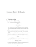
Consumer Theory III:Duality1The Dual Problem1.1Expenditure Minimization1.The expenditure minimization problem:p:xminxs:t:u(x) u;x 0:The solution to this problem tells us the minimum expenditure that is necessary such that the consumer’s utility is not lower than u.2.Solving this problem tells the decision-maker(e.g.the government)the payment necessary to keep a person’s utility above a minimum level.3.De…nitions:A solution to the expenditure minimization problemis known as the Hicksian demand function and is denoted byx h(p;u):Substituting x h(p;u)into the objective function gives us the ex-penditure functione(p;u) p x h(p;u):4.Properties of Hicksian Demand:Suppose u is continuous and strictlyincreasing,then x h has the following properties:(a)Homogeneity of degree zero in p.That is,x h(tp;u)=x h(p;u)for all scalar t>0.(b)No excess utility:u x h(p;u) =u.5.These properties are similar to those of the Marshallian demand.Brie‡y,(a)is obvious from the defn.of the minimization problem;(b)follows from strict monotonicity.6.Theorem:Suppose u is strictly increasing and x h(p;u)is uniquefor all p.Then for any p0and p00;(p00 p0): x h(p00;u) x h(p0;u) 0:7.Proof.We note thatu x h(p00;u) =u x h(p0;u) :By de…nition,x h(p00;u)and x h(p0;u)are the cheapest way to achieve u under p00and p0,respectively.Hencep00 x h(p00;u) p00 x h(p0;u);p0 x h(p0;u) p0 x h(p00;u):These two inequalities imply that(p00 p0): x h(p00;u) x h(p0;u) 0: Note that this result follows entirely from the fact that x h min-imizes expenditure.It does not use any other properties of the utility functions.8.This result is called the compensated law of demand.It statesthat an expenditure-minimizing consumer should substitute low-price goods for high-price goods.Note that if p00and p0di¤er only in the price of good i,then the result becomes(p00i p0i) x h i(p00;u) x h i(p0;u) 0;which means that the Hicksian demand for good i is downward sloping.9.Properties of the Expenditure Function:If u(:)is continuous andstrictly increasing,then the expenditure function e(p;u)has the following properties:(a)Zero when u takes on the lowest level of utility(i.e u(0)whenthe utility function is increasing).(b)Continuous on its domain R n++ U.(c)For all p>>0;strictly increasing and unbounded above in u.(d)Increasing in p.(e)Homogeneous of degree1in p.(f)Concave in p:10.Proof:(a)The consumer can achieve u(0)by not spending anything.(b)Intuitively,the result follows from the continuity of u and thecontinuity of the budget set.(c)This is straightforward.Suppose e is not strictly increasing inu.Then there exist p,u0and u1,u1>u0,such that e(p;u1)e(p;u0).Since u is continuous and strictly increasing in x,itis possible to reduce consumption by some small"such thatu x h(p;u1) " >u0andp:(h(p;u1) ")<e(p;u0):Here"is a vector:This violates the de…nition of e(p;u0).Sup-pose that e is bounded by some e (meaning that e(p;u) efor all p and y).Since e is strictly increasing in u,e(p;v(p;e )+1)must be greater than e ,a contradiction.(d)If p1 p0(that is,p1i p0i for all i),then any consump-tion bundle x that is feasible under p1is also under p0.Sincee(p;u)is by de…nition the lowest expenditure that is neces-sary to achieve u,e p0;u p0x h p1;u p1x h p1;u e p1;u :(e)This immediately follows from the fact the Hicksian demandis homogeneous in degree zero in p.(f)Let x1=x h(p1;u)and x2=x h(p2;u).By de…nition,for anyx such that u(x) ue p1;u =p1x1 p1xande p2;u =p2x2 p2x:It follows that for any t2[0;1]and for any x such thatu(x) ute p1;u +(1 t)e p2;u tp1+(1 t)p2 x:The above equation holds for all x such that u(x) u,in-cluding x h(tp1+(1 t)p2;u).Hence,te p1;u +(1 t)e p2;u tp1+(1 t)p2 x h tp1+(1 t)p2;ue tp1+(1 t)p2 ;u :It is important to note that the concavity of e follows from thede…nition of e and does not require that u be quasiconcave.11.Di¤erentiable Utility.Solving a minimization problem involves thesame technique as solving a maximization problem.However,inthis problem the last equation comes from the utility constraint,whereas in the maximization problem it comes from the budgetconstraint.The Lagrangian function isL=p:x+ (u u(x)):The…rst order conditions are(assuming x>>0):@L @x i =p i @u@xi=0for all i=1;:::;n;@L@=u u(x)=0: The…rst n equations imply@u@x1 p1=::::=@u@x np n12.Shephard’s lemma:If e(p;u)is di¤erentiable in p at(p0;u0)withp0>>0,then@e(p0;u0)@p i=x h i p0;u0 ;i=1;:::;n:The results follows directly from the envelope theorem.@e @p i =@L@p i=x h i.The Shephard’s lemma is the counterpart of Roy’s Identity.Same Intuition.1.2Relationship Between Marshallian and Hick-sian Demand Functions1.The indirect utility function and expenditure function are inti-mately connected.So are the Marshallian and Hicksian demand functions.We have already seen that the two demand functions share a common tangency condition.Regardless of whether one’s objective is to maximize utility or minimize expenditure,one should consume in such a way that the marginal utility per dollar spent on each good is the same.2.Theorem1.8.Let v(p;I)and e(p;u)be the indirect utility func-tion and expenditure function for a consumer with a continuous and strictly increasing utility function.Then(a)e(p;v(p;I))=I;(b)v(p;e(p;u))=u:3.Part1says that if the maximum utility the consumer can obtaingiven p and I is v,then the minimum expenditure needed to achieve v is I.Part2says that if the minimum expenditure needed to achieve utility u given p is e,then maximum utility one can obtain given p and e is u.4.Proof:I will only prove part1.Part2can be proven in the sameway.Since e(p;v(p;I))is by de…nition the minimum expenditure needed to attain v(p;I),it must be that e(p;v(p;I)) I.Suppose e(p;v(p;I))<I.Then,there exists x such that px <I and u(x ) v(p;I).By strict monotonicity,p(x +")<Iand u(x +")>v(p;I)for some small".This contradicts the supposition that v(p;I)is the highest utility attainable given p and I.5.Note that the theorem is incorrect if the utility function is notstrictly increasing.For example:if u(x)=10for all x,thenv(p;5)=10;e(p;10)=0:6.Theorem1.9.Suppose u is continuous,strictly quasiconcave,andstrictly increasing.Then for all p>>0,I 0,and u2U,we have(a)x(p;I)=x h(p;v(p;I)).(b)x h(p;u)=x(p;e(p;u)).7.The…rst relation says that the Marshallian demand at prices pand income I is equal to the Hicksian demand at prices p and the maximum utility level that can be achieved at prices p and incomeI.The second says that the Hicksian demand at any prices pand utility level u is the the same as the Marshallian demand at those prices and an income level equal to the minimum expenditure necessary to achieve the utility level.8.Proof:Strict quasiconcavity means that both x(p;I)and x h(p;u)are unique.To prove part1,note that by Theorem1.8the mini-mum expenditure needed to attain v(p;I)is I.Since u(x(p;I))= v(p;I)(by de…nition of v)and px(p;I)=I,x(p;I)is the solu-tion of the expenditure minimization problem.The proof for the second part is similar.9.There are two ways to derive the Hicksian demand.The direct wayis to solve expenditure minimization problem.But we can also get the marshallian demand by solving the utility maximization problem.Substitute the demand back into the utility function.This gives the indirect utility function.From the indirect utility function,we know how much income need to change to keep utility constant as price change.Substitute this back into the Marshallian demand gives the Hicksian demand.10.Cobb-Douglas example:u(x1;x2)=x 1x 2, + =1x1= Ip1;x2=Ip2The indirect utility function isv(I;p1;p1)=u(x(p1;p2;I);x2(p1;p2;I))= I p1 I p2 = p1 p2 I Rearranging the termse(p x;p y;u)=up1 p2 = p1 p2 u:The Hicksian demand for Cobb-Douglas utility function is x h1= p1 1 p2 u;x h2= p1 p2 1u:1.3An Example:CES(continued)We continue the example u(x1;x2)=(x 1+x 2)1= :We want to derive the corresponding expenditure function,then compare it with the indirect utility function,and show the duality between Marshallian and Hicksian demand functions.1.3.1Expenditure functionBecause the preferences are monotonic,we can formulate the expenditure minimization problem as:minx1;x2p1x1+p2x2subject to:(x 1+x 2)1= =u;x1;x2 0And its LagrangianL(x1;x2; )=p1x1+p2x2+ [u (x 1+x 2)1= ] Assuming the interior solution in both goods,and by the…rst-order condition we have:@L@x1=p1 (x 1+x 2)(1= ) 1x 11=0@L@x2=p2 (x 1+x 2)(1= ) 1x 12=0@L@=u (x 1+x 2)1= =0By the…rst two,we can getx1=x2 p1p2 1=( 1)By the third one,we haveu=(x 1+x 2)1=1.3.2Hicksian demandsBy the above two equations,we can get the Hicksian demandsx h1(p;u)=u(p r1+p r2)(1=r) 1p r 11;x h2(p;u)=u(p r1+p r2)(1=r) 1p r 12where r= =( 1):1.3.3Expenditure functionTherefore,we can obtain the expenditure function:e(p;u)=p1x h1(p;u)+p2x h2(p;u)=u(p r1+p r2)1=r:1.3.4Relationship between indirect utility and expenditurefunctionsThey actually imply each other.When you get one,you can get the other very quickly.In previous lecture,we’ve already got the indirect utility function:v(p;I)=I(p r1+p r2) 1=r:For income level I=e(p;u);we must havev(p;e(p;u))=e(p;u)(p r1+p r2) 1=rWe’ve already know from theorem1.8,that v(p;e(p;u))=u;there-fore we haveu=e(p;u)(p r1+p r2) 1=rWe can get the expenditure functione(p;u)=u(p r1+p r2)1=rAnd you can try to get the indirect utility function given the expen-diture function is known.1.3.5Relationship between Marshallian and Hicksian demands We know the Marshallian demands in the previous lecture asx i(p;I)=p r 1iIp r1+p r2;i=1;2;x i(p;e(p;u))=e(p;u)p r 1ip r1+p r2=u(p r1+p r2)(1=r) 1p r 1i=x h i(p;u)2Income and Substitution E¤ects1.Slutsky equation:sincex h i(p;u )=x i(p;e(p;u ))@x h i(p;u )@p j =@x i(p;I)@p j+@x i(p;I)@I@e(p;u )@p j=@x i(p;I)@p j+@x i(p;I)@Ix h j(p;u )(by Sheppard’s lemma) =@x i(p;I)@p j+x j(p;I)@x i(p;I)@IRearranging the terms,we have@x i(p;I)@p j =@x h i(p;u )@p j x j(p;I)@x i(p;I)@I(1)The Slutsky equation decompose the e¤ect of the price of good j on the quantity demand of good i into a substitution e¤ect and an income e¤ect.The former captures the e¤ect of relative price,and the latter the e¤ect of purchasing power.To separate the income e¤ect from the substitution e¤ect,we can imagine that the consumers are compensated for the change in purchasing power due to a change in price so that their utility remain unchanged,and study how their demand for a good will change purely as a result of relative price changes.Hence,the Hicksian demand is also called the compensated demand,and the Marshallian Demand uncompensated demand.From the theorem,we certainly have@x i(p;I)@p i =@x h i(p;u )@p i x i(p;I)@x i(p;I)@I@x h i(p;u )i 0.The reason is because the expenditure function is a concave function of p;therefore we have@2e(p;u)@p2i =@x h i(p;u)@piThe income e¤ect can be positive or negative.Thus,(1)tells that for normal goods(@x i>0),@x i @p j <@x h i@p jmeaning that the Marshallian demand has a‡atter slope.The opposite is true for inferior goods.2.1The Slutsky Substitution Matrix1.Given a Marshallian demand function x (p;I ),let s ij@x i (p;I )@p j +x j (p;I )@x i (p;I )@I :2.The Slutsky matrix is de…ned as 266664s 11s 12::s 1n s 21:::::s n 1s nn3777753.Theorem:Suppose x (p;I )is a Marshallian demand function gener-ated by some continuous,strictly increasing utility function.Then the Slutsky matrix of x is symmetric and negative semide…nite.4.Proof:The proof is not hard,but it makes use of several results that we have just learnt.From the Slutsky equation,we haves ij =@x h i @p j:(The reason we need the utility function to be strictly increasing or at least locally non-satiated,is that without it Theorem 1.9and,hence,the Slutsky equation does not hold.)By the Sheppard’s lemma,we have for any i and j@2e @p i @p j =@x h i @p j =@x h j @p i:This implies that the Slutsky matrix is symmetric.Finally,since e is concave,its Hessian matrix:26666664@x h 1@p 1@x h 1@p 2::@x h 1@p n @x h 2@p 1:::::@x h 1@p n @x h n @p n37777775must be negative semide…nite.2.2Compensating Variation and Consumer Surplus1.When the government decides whether to cut or raise sales taxes,it has to know how will the tax a¤ect consumer welfare.In an-titrust law suit,an important factor that the court will look into is whether consumers are hurt by the monopolist.2.The expenditure function provides us a formal way to measurehow a change in price a¤ects consumer welfare.De…nition:Com-pensating variation(CV)associated with a change in the price of good i is the income compensation required to keep the utility ofa consumer constant.That is,CV e(p0i;p i;u) e(p i;p i;u):Or,alternatively,v(p0i;p i;I+CV)=v(p i;p i;I):By Shephard’s Lemma,@e@p i=x h.It follows thatCV=Z p0i p i@e@p i dp i;=Z p0i p i x h(p i;p i;u)dp i:Thus,the compensating variation is the area to the left of the Hicksian demand between p i and p0i.(Draw diagram)This is an extremely important result because it allow us to evaluate the wel-fare consequence of a policy.3.Since Hicksian demand is not directly observable,it is more con-venient to measure welfare change using Marshallian rather than Hicksian demand.The consumer surplus(at p i),CS,is the area bound by the Marshallian demand and p i.The change in CS when the price of good i changes from p i to p0i is4CS=Z p i p0i x(p i;p i;I)dp i:Recall from the Slutsky equation that@x i@p j p;I=@x h i@p j p;v(p;I) @x i@I p;I x i(p;I): 11For normal goods,x i(p0i;I)<x h i p0i;v(p i;p i;I) when p0i>p i, that is,Marshallian demand decreases more when it is a price increase.x i(p0i;I)>x h i p0i;v(p i;p i;I) when p0i<p i,that is, Marshallian demand increases more when price goes down.The converse is true for inferior goods.Hence,for normal goodsj4CS j>j CV jif price decreases,andj4CS j<j CV jwhen price increases.For normal goods,the change in consumer surplus underestimates the welfare loss due to price increase and overestimate the welfare gain due to a price decrease.4.Although,j4CS j=j CV j,in practice the di¤erence is pretty smalland is insigni…cant compared to measurement errors.12。

微观经济学讲义摘要：其中下划线标注的文字，公式，图表部分是从课堂笔记中得知的重点，是必须掌握的（但其余部分绝不能排除重点与考点的存在，包括超出讲义范围的可能性）。

第一章 绪论1-1， 什么是经济学经济学是研究个人和团体从事生产、交换以及对产品和服务消费的一种社会科学，它研究怎样最佳使用稀缺的资源以满足人们无限的需求。

1-2， 经济学的基本研究方法可以分为以下四种：个量与总量分析法，静态与动态分析法， 定性与定量分析法，实证与规范分析法1-3， 实证经济学（Positive Economics ）是用理论对社会各种经济活动或经济现象进行解释、分析、证实或预测。

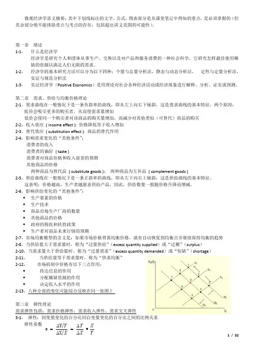
第二章 需求、供给与均衡价格理论2-1，需求曲线在一般情况下是一条负斜率的曲线，即从左上向右下倾斜，这是需求曲线的基本特征，两个原因：低价会吸引更多的购买者，从而使需求量增加低价会使同一个购买者对该商品的购买量增加，而减少对其他类似（可替代）商品的购买2-2，收入效应 ( income effect ): 价格降低等于收入增加2-3，替代效应 ( substitution effect ): 商品的替代作用2-4，影响需求变化的“其他条件”：消费者的收入消费者的偏好 ( taste )消费者对商品价格和收入前景的预期其他商品的价格两种商品为替代品 ( substitute goods )； 两种商品为互补品 ( complement goods )2-5，供给曲线在一般情况下是一条正斜率的曲线，即从左下向右上倾斜，这是供给曲线的基本特征。

这表明：价格越高，生产者越愿意供给产品，因此，供给数量一般随价格升降而增减。

2-6，影响供给变化的“其他条件”：▪ 生产要素的价格▪ 生产技术▪ 商品市场生产厂商的数量▪ 其他商品的价格▪ 政府的税收和扶持政策▪ 生产者对商品未来行情的预期2-7，市场均衡模型的含义是：如果市场价格背离均衡价格，就有自动恢复到均衡点并继续保持均衡的趋势 2-8，当供给量大于需求量时，称为“过量供给”（excess quantity supplied ）或“过剩”（surplus ）2-10，当需求量大于供给量时，称为“过量需求”（excess quantity demanded ）或“短缺”（shortage ）2-11， 当供给量等于需求量时，称为“供求均衡”2-12， 市场机制中价格有以下三点作用：▪ 传达信息的作用▪ 分配稀缺资源的作用▪ 决定收入水平的作用2-13，八种全部的变化可能综合反映在同一张图上第三章 弹性理论需求弹性包括：需求价格弹性，需求收入弹性，需求交叉弹性3-1， 弹性：因变量变化的百分比同自变量变化的百分比之间的比例关系弹性系数 X Y Y •∆=∆=Y e3-2， 需求价格弹性 ( price elasticity of demand ) ：是需求量的变动对价格变动的敏感程度 注意：需求价格弹性系数值当为负值。