中国移动实现TD城区面积覆盖率80%

MALDIquant:Quantitative Analysis of MassSpectrometry DataSebastian Gibb*March20,2023AbstractMALDIquant provides a complete analysis pipeline for MALDI-TOF and other2D mass spectrometry data.This vignette describes the usage of the MALDIquant package andguides the user through a typical preprocessing workflow.**********************1Contents1Introduction3 2Setup3 3MALDIquant objects3 4Workflow44.1Data Import (6)4.2Quality Control (7)4.3Variance Stabilization (9)4.4Smoothing (9)4.5Baseline Correction (9)4.6Intensity Calibration/Normalization (11)4.7Warping/Alignment (11)4.8Peak Detection (12)4.9Peak Binning (14)4.10Feature Matrix (14)5Summary15 6Session Information15 ForewordMALDIquant is free and open source software for the R(R Core Team,2014) environment and under active development.If you use it,please support the project by citing it in publications:Gibb,S.and Strimmer,K.(2012).MALDIquant:a versatile Rpackage for the analysis of mass spectrometry data.Bioinformat-ics,28(17):2270–2271If you have any questions,bugs,or suggestions do not hesitate to contact me(*********************).Please visit http://strimmerlab.github.io/software/maldiquant/.21IntroductionMALDIquant comprising all steps from importing of raw data,preprocessing (e.g.baseline removal),peak detection and non-linear peak alignment to calibration of mass spectra.MALDIquant was initially developed for clinical proteomics using Matrix-Assisted Laser Desorption/Ionization(MALDI)technology.However,the algorithms implemented in MALDIquant are generic and may be equally ap-plied to other2D mass spectrometry data.MALDIquant was carefully designed to be independent of any specific mass spectrometry hardware.Nonetheless,a lot of open and nativefile formates, e.g.binary datafiles from Brukerflex series instruments,mzXML,mzML, etc.are supported through the associated R package MALDIquantForeign. 2SetupAfter starting R we could install MALDIquant and MALDIquantForeign di-rectly from CRAN using install.packages:>install.packages(c("MALDIquant","MALDIquantForeign")) Before we can use MALDIquant we have to load the package.>library("MALDIquant")3MALDIquant objectsMALDIquant is written in an object-oriented programming approach and uses R’s S4objects.A spectrum is represented by an MassSpectrum and a list of peaks by an MassPeaks instance.To create such objects manually we could use createMassSpectrum and createMassPeaks.In general we do not need these functions because MALDIquantForeign’s import routines will generate the MassSpectrum/MassPeaks objects.3>s<-createMassSpectrum(mass=1:10,intensity=1:10,+metaData=list(name="Spectrum1"))>sS4class type:MassSpectrumNumber of m/z values:10Range of m/z values:1-10Range of intensity values:1-10Memory usage:1.414KiBName:Spectrum1Each MassSpectrum/MassPeaks stores the mass and intensity values of a spectrum respective of the peaks.Additionally they contain a list of meta-data.To access these information we use mass,intensity and metaData. >mass(s)[1]12345678910>intensity(s)[1]12345678910>metaData(s)$name[1]"Spectrum1"4WorkflowA Mass Spectrometry Analysis often follows the same workflow(see also Fig.1).After importing the raw data(see also the MALDIquantForeign package) we control the quality of the spectra and draw some plots.We apply a variance-stabilizing transformation and smoothingfilter.Next we remove the chemical background using a Baseline Correction method.To compare4the intensities across spectra we calibrate the intensity values(often called normalization)and the mass values(warping,alignment).Subsequently we perfom a Peak Detection and do some post processing likefiltering etc.Figure1:MS Analysis Workflow54.1Data ImportNormally we will use some of the import methods provided by MALDIquantForeign,e.g.importBrukerFlex,importMzMl,etc.But in this vignette we will usea small example dataset shipped with MALDIquant.This dataset is a subsetof MALDI-TOF data described in Fiedler et al.(2009).>data(fiedler2009subset)fiedler2009subset is a list of16MassSpectrum objects.The16spec-tra are8biological samples with2technical replicates.>length(fiedler2009subset)[1]16>fiedler2009subset[1:2]$sPankreas_HB_L_061019_G10.M19.T_0209513_0020740_18S4class type:MassSpectrumNumber of m/z values:42388Range of m/z values:1000.015-9999.734Range of intensity values:5-101840Memory usage:506.359KiBName:Pankreas_HB_L_061019_G10.M19File:/data/set A-discovery leipzig/control/Pankreas_HB_L_0 $sPankreas_HB_L_061019_G10.M20.T_0209513_0020740_18S4class type:MassSpectrumNumber of m/z values:42388Range of m/z values:1000.015-9999.734Range of intensity values:6-111862Memory usage:506.359KiBName:Pankreas_HB_L_061019_G10.M20File:/data/set A-discovery leipzig/control/Pankreas_HB_L_064.2Quality ControlFor a basic quality control we test whether all spectra contain the same number of data points and are not empty.>any(sapply(fiedler2009subset,isEmpty))[1]FALSE>table(sapply(fiedler2009subset,length))4238816Subsequently we control the mass difference between each data point (should be equal or monotonically increasing)because MALDIquant is de-signed for profile data and not for centroided data.>all(sapply(fiedler2009subset,isRegular))[1]TRUEFinally we draw some plots and inspect the spectra visually.>plot(fiedler2009subset[[1]])7>plot (fiedler2009subset[[16]])200040006000800010000050001500Pankreas_HB_L_061019_D9.G18/data/set B − discovery heidelberg/tumor/Pankreas_HB_L_061019_D9/0_g18/1/1SLin/fidm zi n t e n s i t y84.3Variance StabilizationWe use the square root transformation to simplify graphical visualization and to overcome the potential dependency of the variance from the mean. >spectra<-transformIntensity(fiedler2009subset,+method="sqrt")4.4SmoothingNext we use a21point Savitzky-Golay-Filter(Savitzky and Golay,1964)to smooth the spectra.>spectra<-smoothIntensity(spectra,method="SavitzkyGolay", +halfWindowSize=10)4.5Baseline CorrectionBefore we correct the baseline we visualize it.Here we use the SNIP algorithm (Ryan et al.,1988).>baseline<-estimateBaseline(spectra[[16]],method="SNIP",+iterations=100)>plot(spectra[[16]])>lines(baseline,col="red",lwd=2)9200040006000800010000050100150Pankreas_HB_L_061019_D9.G18/data/set B − discovery heidelberg/tumor/Pankreas_HB_L_061019_D9/0_g18/1/1SLin/fidm zi n t e n s i tyIf we are satisfied with our estimated baseline we remove it.>spectra <-removeBaseline (spectra,method ="SNIP",+iterations =100)>plot (spectra[[1]])1020004000600080001000005010015020025Pankreas_HB_L_061019_G10.M19/data/set A − discovery leipzig/control/Pankreas_HB_L_061019_G10/0_m19/1/1SLin/fid m z i n t e n s i t y4.6Intensity Calibration/NormalizationFor better comparison and to overcome (very)small batch effects we equal-ize the intensity values using the Total-Ion-Current-Calibration (often called normalization).>spectra <-calibrateIntensity (spectra,method ="TIC")4.7Warping/AlignmentNow we (re)calibrate the mass values.Our alignment procedure is a peak based warping algorithm.If you need a finer control or want to investigate the impact of different parameters please use determineWarpingFunctions instead of the easier alignSpectra .>spectra <-alignSpectra (spectra,+halfWindowSize =20,+SNR =2,+tolerance =0.002,+warpingMethod ="lowess")11Before we call the Peak Detection we want to average the technical repli-cates.Therefore we look for the sample name that is stored in the metadata because each technical replicate has the same sample name.>samples<-factor(sapply(spectra,+function(x)metaData(x)$sampleName)) Next we use averageMassSpectra to create a mean spectrum for each biological sample.>avgSpectra<-averageMassSpectra(spectra,labels=samples,+method="mean")4.8Peak DetectionThe next crucial step is the Peak Detection.Before we perform the peak detection algorithm we estimate the noise of the spectra to get a feeling for the signal-to-noise ratio.>noise<-estimateNoise(avgSpectra[[1]])>plot(avgSpectra[[1]],xlim=c(4000,5000),ylim=c(0,0.002)) >lines(noise,col="red")>lines(noise[,1],noise[,2]*2,col="blue")124000420044004600480050000.00000.00100.0020Pankreas_HB_L_061019_A6.A11Pankreas_HB_L_061019_A6.A12averaged spectrum composed of 2 MassSpectrum objectsm z i n t e n s i t yWe decide to use a signal-to-noise ratio of 2(blue line).>peaks <-detectPeaks (avgSpectra,method ="MAD",+halfWindowSize =20,SNR =2)>plot (avgSpectra[[1]],xlim =c (4000,5000),ylim =c (0,0.002))>points (peaks[[1]],col ="red",pch =4)134000420044004600480050000.00000.00100.0020Pankreas_HB_L_061019_A6.A11Pankreas_HB_L_061019_A6.A12averaged spectrum composed of 2 MassSpectrum objectsm z i n t e n s i t y4.9Peak BinningAfter the alignment the peak positions (mass)are very similar but not iden-tical.The binning is needed to make similar peak mass values identical.>peaks <-binPeaks (peaks,tolerance =0.002)4.10Feature MatrixWe choose a very low signal-to-noise ratio to keep as much features as pos-sible.To remove some false positive peaks we remove less frequent peaks.>peaks <-filterPeaks (peaks,minFrequency =0.25)At the end of the analysis we create a feature matrix that could be used in further statistical analysis.Please note that missing values (not detected peaks)are imputed/interpolated from the corresponding spectrum.14>featureMatrix<-intensityMatrix(peaks,avgSpectra)>head(featureMatrix[,1:3])1011.731822275831020.67480821711029.40115131151[1,]0.00018949470.00077159870.0001093035[2,]0.00021443540.00150305600.0001422394[3,]0.00021171470.00045556880.0001303326[4,]0.00023141810.00052609770.0001441254[5,]0.00015624010.00240540310.0001198008[6,]0.00016006300.00203151910.00010904845SummaryWe shortly described a complete example workflow of a mass spectrometry data analysis.Please note that this workflow is only an example and could not cover every use case.MALDIquant provides a lot of more functions than we mentioned in this vi-gnette.The described functions are the most used ones but they have a lot of more parameters which could/need adjust to your data(e.g.halfWindowSize, SNR,tolerance,etc.).That’s why we suggest the user to read the manual pages of theses functions carefully.We also provide more examples in the demo directory and at:http://strimmerlab.github.io/software/maldiquant/Please do not hesitate to contact me(*********************)if you have any questions.6Session InformationR version4.2.3(2023-03-15),x86_64-pc-linux-gnuRunning under:Debian GNU/Linux11(bullseye)Matrix products:defaultBLAS:/usr/lib/x86_64-linux-gnu/blas/libblas.so.3.9.015LAPACK:/usr/lib/x86_64-linux-gnu/lapack/liblapack.so.3.9.0Base packages:base,datasets,grDevices,graphics,methods,stats,utilsOther packages:MALDIquant1.22.1,knitr1.42Loaded via a namespace(and not attached):compiler4.2.3,evaluate0.20,highr0.10,parallel4.2.3,tools4.2.3,xfun0.37 ReferencesFiedler,G.M.,Leichtle,A.B.,Kase,J.,Baumann,S.,Ceglarek,U.,Felix, K.,Conrad,T.,Witzigmann,H.,Weimann,A.,Sch¨u tte,C.,Hauss,J., B¨u chler,M.,and Thiery,J.(2009).Serum peptidome profiling revealed platelet factor4as a potential discriminating peptide associated with pan-creatic cancer.Clin Cancer Res,15(11):3812–3819.Gibb,S.and Strimmer,K.(2012).MALDIquant:a versatile R package for the analysis of mass spectrometry data.Bioinformatics,28(17):2270–2271. R Core Team(2014).R:A Language and Environment for Statistical Com-puting.R Foundation for Statistical Computing,Vienna,Austria. Ryan,C.,Clayton,E.,Griffin,W.,Sie,S.,and Cousens,D.(1988).Snip, a statistics-sensitive background treatment for the quantitative analysis of pixe spectra in geoscience applications.Nuclear Instruments and Meth-ods in Physics Research Section B:Beam Interactions with Materials and Atoms,34(3):396–402.Savitzky,A.and Golay,M.J.E.(1964).Smoothing and differentiation of data by simplified least squares procedures.Analytical Chemistry, 36(8):1627–1639.16。

Agilent Protein 80 Kit, Part Number 5067-1515*************(24小时)化学品安全技术说明书GHS product identifier 应急咨询电话（带值班时间）::供应商/ 制造商:安捷伦科技贸易（上海）有限公司中国（上海）外高桥自由贸易试验区英伦路412号（邮编:200131)电话号码： 800-820-3278传真号码: 0086 (21) 5048 2818Agilent Protein 80 Kit, Part Number 5067-1515化学品的推荐用途和限制用途物质用途:分析试剂。

研究和开发Protein 80 Gel MatrixProtein 80 Gel Matrix 4 x 0.65 ml（毫升）Protein 80 Dye ConcentrateProtein 80 Dye Concentrate 1 x 0.09 ml（毫升）Protein 80 Sample BufferProtein 80 Sample Buffer 4 x 0.2 ml（毫升）Protein 80 LadderProtein 80 Ladder 1 x 0.18 ml（毫升）安全技术说明书根据 GB/ T 16483-2008 和 GB/ T 17519-2013GHS化学品标识:安捷伦蛋白80试剂盒，部件号 5067-1515物质或混合物的分类根据 GB13690-2009 和 GB30000-2013紧急情况概述Protein 80 Gel Matrix 液体。

Protein 80 Dye Concentrate 液体。

Protein 80 Sample Buffer 液体。

Protein 80 Ladder 液体。

Protein 80 Gel Matrix 无资料。

Protein 80 Dye Concentrate 蓝色。

Protein 80 Sample Buffer 无资料。

八十岁老人血脂标准
八十岁老人的血脂标准通常会有一些变化，因为随着年龄的增长，人体的新陈代谢和生理功能也会发生变化。

血脂是指血液中的
脂质类物质，包括胆固醇和甘油三酯等，它们对心血管健康有重要
影响。

在八十岁的老年人群中，一般来说，对血脂标准的评估会更
加谨慎和个体化。

在八十岁老人中，总胆固醇的标准范围可能会有所扩大，因为
一些研究表明，较高的胆固醇水平可能与更长寿命相关联。

然而，
这并不意味着高胆固醇就是安全的，因为它仍然与心血管疾病的风
险增加相关。

一般来说，八十岁老人的总胆固醇水平应该控制在
190毫克/分升以下。

对于LDL（低密度脂蛋白）胆固醇，或称为“坏”胆固醇，八
十岁老人的标准范围可能会有所放宽，但仍然需要控制在较低水平。

一般来说，LDL胆固醇水平应该控制在100毫克/分升以下。

而对于HDL（高密度脂蛋白）胆固醇，或称为“好”胆固醇，
八十岁老人的标准范围可能会有所提高，因为高水平的HDL胆固醇
与心血管保护有关。

一般来说，HDL胆固醇水平应该保持在40毫克
/分升以上。

另外，甘油三酯是血液中的另一种重要脂质成分，对心血管健康也有影响。

八十岁老人的甘油三酯水平应该控制在150毫克/分升以下。

需要指出的是，以上所述的血脂标准仅供参考，实际标准可能会因个体差异、患有其他疾病或接受药物治疗等因素而有所不同。

因此，针对八十岁老人的血脂管理，建议还是应该由专业医生根据个体情况进行评估和制定合理的管理方案。

同时，老年人在控制血脂的过程中，也应该注意合理饮食、适量运动和定期体检等综合措施，以维护心血管健康。

a验胆固醇量度有两种单位，一种单位是mmol/l，总胆固醇量度5.2mmol/L或以下为正常。

另一单位是mg/dl ，总胆固醇量度200mg/dl以下为正常。

医学界认为，为了降低胆固醇，也应该减少一些含高胆固醇食物的摄取，尤其是心、肝等动物内脏。

蛋类每星期以不超过三四个为原则，尤其尽量少吃蛋黄，包括各种鱼卵、蟹黄等。

烹调用油应采用植物油，此外，也必须限制醣量，最好禁止食用纯糖类食品或饮料。

尽量少吃全脂牛奶、巧克力奶、奶油及各种乳酪，多吃脱脂奶及豆浆。

肉类方面，应该禁吃肥肉、猪皮、蹄膀、香肠，及各种有油的牛羊猪肉等。

海鲜方面则应避免虾、蟹、蚌、牡蛎。

此外，各种精致甜点如蛋糕、巧克力仅量少吃。

各种动物油脂、椰子油等应禁食，以人造黄油及植物油取代。

不含胆固醇的食物日常饮食中其实有许多不含胆固醇的食物，包括硬壳果类，如杏仁、核桃；五谷类、蛋白，水果类果酱、果冻；此外，还有蔬菜类、花生、花生酱，植物性油脂及人造奶油、面筋、豆类与豆浆、豆腐等豆制品。

尤其多吃水果，水果含果胶，也能降低胆固醇。

近年来有不少报告显示，摄取燕麦也能降低胆固醇。

许多研究显示，燕麦其实和豆类同样有效，如果每天在低脂饮食中添加两三杯燕麦片，其降低胆固醇的效果较仅采取健康饮食还好。

其他有益于降低胆固醇的食物还有胡萝卜及生蒜头。

过去有不少研究显示，摄取大量的生蒜头能减少有害的血脂肪。

除了饮食外，规律运动及体重控制均有助于降低体内胆固醇不管是胆固醇或三酸甘油脂过高，患者都应该少吃油脂，特别是猪油、牛油等含有高饱和脂肪酸者，宜改用多元不饱和脂肪酸油脂，如葵花油、大豆油、玉米油等。

胆固醇偏高的人，除了少吃脑、肝、腰子、肠子、蛋黄（每周不超过二至三个）、蟹黄及猪皮、鸡皮、鱼皮等食物，并要减少甜食，因为糖分是合成胆固醇的原料；至于三酸甘油脂偏高的人，特别要注意不能饮酒、咖啡，不能吃甜度太高的水果。

多食用富含纤维的食物，如蔬菜、谷类、海藻和菇菌类，可帮忙降低胆固醇，此外，如干豆类、燕麦麸皮、生洋葱、大蒜、胡萝卜、苹果、酪梨、核桃、秋刀鱼等也是不错的选择。

febuxostat 80 的用法-回复关于febuxostat 80的用法Febuxostat（商品名为Uloric）是一种用于治疗高尿酸血症的药物。

高尿酸血症是指体内尿酸含量过高，可以导致痛风以及尿酸结晶引起的肾结石等疾病。

Febuxostat 80是一种含有80毫克febuxostat成分的药物，用于控制和减少血液中的尿酸水平。

尿酸是由体内新陈代谢过程中产生的废物，通常通过肾脏排出体外。

然而，对于某些人来说，体内产生过多的尿酸或肾脏无法有效地排出尿酸，导致尿酸在体内积累过多。

这就是高尿酸血症的发生。

高尿酸血症可以导致痛风，痛风是一种关节炎，特征是突发性的关节疼痛、红肿和热感。

尿酸结晶也可能形成肾结石，引发肾脏疾病。

因此，控制尿酸水平对于预防和治疗这些疾病非常重要。

Febuxostat 80是一种可以降低体内尿酸水平的处方药物。

它通过抑制尿酸合成的酶（xanthine oxidase）的活动，降低体内尿酸的产生。

请注意，这种药物只用于治疗已经被确诊为高尿酸血症的患者，因此在使用之前需要医生的明确诊断和建议。

以下是使用Febuxostat 80的一般步骤：1. 医生咨询：首先，您需要向您的医生咨询，申请开具febuxostat 80的处方。

医生将会根据您的情况评估该药物是否适合您以及确定正确的剂量。

2. 开具处方：一旦确定了适应症，医生将会给您开具一份正式的处方。

请确保您按照医生的指示执行。

3. 药物购买：凭处方，您可以到药房购买febuxostat 80。

请确保您从可信赖的药房购买正品药物。

4. 服用方法：Febuxostat 80作为口服药物，您应该按照医生的建议进行服用。

一般情况下，每天服用1次。

5. 遵循剂量：对于Febuxostat 80，通常建议的剂量为每天80毫克。

但请注意，剂量可能因个体差异而有所调整，因此请严格遵循医生的指示。

6. 注意事项：在服用Febuxostat 80期间，有几个重要的注意事项需要遵守。

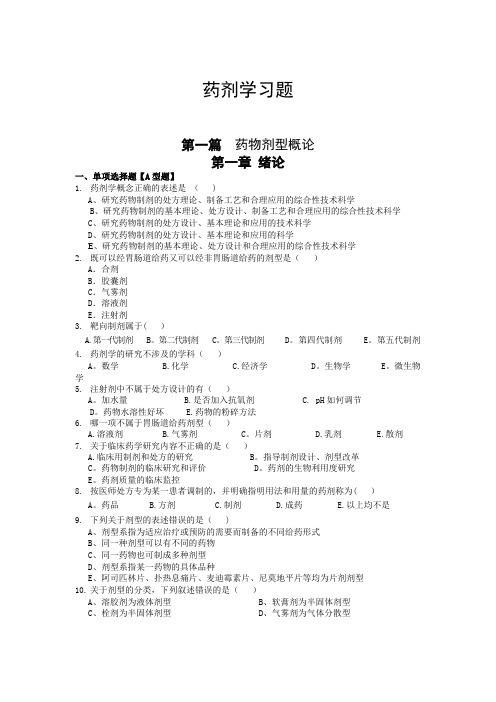
药剂学习题第一篇药物剂型概论第一章绪论一、单项选择题【A型题】1.药剂学概念正确的表述是（ )A、研究药物制剂的处方理论、制备工艺和合理应用的综合性技术科学B、研究药物制剂的基本理论、处方设计、制备工艺和合理应用的综合性技术科学C、研究药物制剂的处方设计、基本理论和应用的技术科学D、研究药物制剂的处方设计、基本理论和应用的科学E、研究药物制剂的基本理论、处方设计和合理应用的综合性技术科学2.既可以经胃肠道给药又可以经非胃肠道给药的剂型是（）A．合剂B．胶囊剂C．气雾剂D．溶液剂E．注射剂3.靶向制剂属于( ）A.第一代制剂 B。

第二代制剂 C。

第三代制剂 D。

第四代制剂 E。

第五代制剂4.药剂学的研究不涉及的学科（）A。

数学 B.化学 C.经济学 D。

生物学 E。

微生物学5.注射剂中不属于处方设计的有（）A。

加水量 B.是否加入抗氧剂 C. pH如何调节D。

药物水溶性好坏 E.药物的粉碎方法6.哪一项不属于胃肠道给药剂型（）A.溶液剂B.气雾剂 C。

片剂 D.乳剂 E.散剂7.关于临床药学研究内容不正确的是（）A.临床用制剂和处方的研究 B。

指导制剂设计、剂型改革C。

药物制剂的临床研究和评价 D。

药剂的生物利用度研究E。

药剂质量的临床监控8.按医师处方专为某一患者调制的，并明确指明用法和用量的药剂称为( ）A。

药品 B.方剂 C.制剂 D.成药 E.以上均不是9.下列关于剂型的表述错误的是（ )A、剂型系指为适应治疗或预防的需要而制备的不同给药形式B、同一种剂型可以有不同的药物C、同一药物也可制成多种剂型D、剂型系指某一药物的具体品种E、阿司匹林片、扑热息痛片、麦迪霉素片、尼莫地平片等均为片剂剂型10.关于剂型的分类，下列叙述错误的是（）A、溶胶剂为液体剂型B、软膏剂为半固体剂型C、栓剂为半固体剂型D、气雾剂为气体分散型E、气雾剂、吸入粉雾剂为经呼吸道给药剂型11.《中华人民共和国药典》是由（）A 国家药典委员会制定的药物手册B 国家药典委员会编写的药品规格标准的法典C 国家颁布的药品集D 国家药品监督局制定的药品标准E 国家药品监督管理局实施的法典12.关于药典的叙述不正确的是( ）A．由国家药典委员会编撰B．由政府颁布、执行，具有法律约束力C．必须不断修订出版D．药典的增补本不具法律的约束力E．执行药典的最终目的是保证药品的安全性与有效性13.药典的颁布，执行单位( ）A.国学药典委员会B.卫生部 C。

HLB值HLB值：表面活性剂为具有亲水基团和亲油基团的两亲分子,表面活性剂分子中亲水基和亲油基之间的大小和力量平衡程度的量,定义为表面活性剂的亲水亲油平衡值。

目录HLB值简介1949年由W.C.Griffin 率先提出HLB值论点,说明表面活性剂分子中的亲水基团与亲油基团的平衡关系。

在HLB中H"Hydrophile" 表示亲水性，L为"Lipophylic"表示亲油性，B 是"Balance"表示平衡的意思。

表面活性剂的亲油或亲水程度可以用HLB值的大小判别，HLB值越大代表亲水性越强，HLB值越小代表亲油性越强，一般而言HLB值从1 ~ 40之间。

HLB在实际应用中有重要参考价值。

亲油性表面活性剂HLB较低,亲水性表面活性剂HLB较高。

亲水亲油转折点HLB 为10。

HLB小于10为亲油性,大于10为亲水性。

HLB值（Hydrophile-Lipophile Balance Number）称亲水疏水平衡值，也称水油度。

它既与表面活性剂的亲水亲油性有关，又与表面活性剂的表面（界面）张力、界面上的吸附性、乳化性及乳状液稳定性、分散性、溶解性、去污性等基本性能有关，还与表面活性剂的应用性能有关。

亲水亲油平衡值（HLB 值）是用来表示表面活性剂亲水或亲油能力大小的值。

1949 年Griffin 提出了HLB 值的概念。

将非离子表面活性剂的HLB 值的范围定为0 ～20 ，将疏水性最大的完全由饱和烷烃基组成的石蜡的HLB 值定为0 ，将亲水性最大的完全由亲水性的氧乙烯基组成的聚氧乙烯的HLB 值定为20 ，其他的表面活性剂的HLB 值则介于0 ～20 之间。

HLB 值越大，其亲水性越强，HLB 值越小，其亲油性越强。

随着新型表面活性剂的不断问世，已有亲水性更强的品种应用于实际，如月桂醇硫酸钠的HLB 值为40 。

HLB=亲水基的亲水性/亲油基的亲油性编辑本段胶束的结构表面活性剂由于在油- 水界面上的定向排列而具有降低界面张力的作用，所以其亲水与亲油能力应适当平衡。

Turbine FlowmeTers wiTh local DigiTal DisplayFTB790 SeriesFTB790 Series turbine meters with microprocessor-based electronics offers a durable, compact, high-precision fluidmeasurement device, with total and rate indication. Information is clearly displayed on a large 6-digit liquid crystal display with only 2-point floating decimal for totals from 0.01 to 999,999. All operations are easily performed with only 2 buttons. The basic unit and display are powered by 2 lithium batteries, providing up to 5 years of use. Cumulative total, batch total, and rate of flow are standard. A single-point field calibration curve can be stored in memory. The turbine meter can also beordered without displayelectronics. A special pulseoutput model (FLSC790-P-ND)must be ordered to obtain an open collector current sinking outputoperated on 9 to 35 Vdc. Theoutput is a square wave pulsewith a 3-wire connection.Accessories for Turbine Meters With the Display: The FLSC790-MA provides a 4 to 20 mA or 0 to 5 Vdc output for rate indication. The output module requires field calibration. The 4 to 20 mA dc is a 2-wire system requiring 8 to 30 Vdc power (24 Vdc recommended).The FLSC790-P pulse outputmodule provides an unscaled open collector sinking output operatingon an applied voltage of 0 to 60 Vdc. The output is a square wave pulse with an amplitude the same as the supplied voltage. The FTB790-RK remote kit allows remote mounting of display electronics. This option expands the applications into wider fluidtemperature ranges to -40 to 121°C (-40 to 250°F). The LCD display can be mounted up to 90 m (300') from the turbine meter.The FLSC790-90D is a 90°mounting adaptor designed to allow displays to be mounted 90° from the standard position.G2S20N09GMBG2S15N09GMBG2S05N09GMAG2S07N09GMAG2S10N09GMAAll models shown smaller than actual size.F-61U I ndicates Both Rate and Total UU p to 1% Reading AccuracyU 6-Digit Display U S ignal Output Capabilities UG PM or LPM (Field Selectable)UB attery Operated (Included)U P VDF (FTB890) or PVC (FTB690) ModelsAlso Available** Extended low flow range and field calibration for viscosity not available on “-ND ” (no display) units.For units with ISO threads add “-ISO” to the model number, for additional cost.For units with T ri-Grip mounting add “-TRI” to model number, for additional cost.For high pressure units [207 bar (3000 psig)], add suffix “-HP” to model number, for additional cost.SPECIFICATIONSAccuracy:G2S05N09GMA : ±2% rdg G2S07N09GMA,G2S10N09GMA : ±1.5% rdg G2S15N09GMB,G2S20N09GMB : ±1.0% rdgExtended Low Flow Range Accuracy: ±5.0% of reading (display models only)Repeatability: ±0.1%Pressure Rating: 1500 psig (103 bar)With “-HP” Option: 3000 psig (207 bar)Except as noted, options and accessories are for display models only. Only one module can be installed per unit. Comes complete with two 3V lithium batteries and operator’s manual.† Comes complete with 3 m (10') cable, and operator’s manual.Ordering Examples: G2S10N09GMA , 1" turbine meter, with FLSC790-MA , field installable 4 to 20 mA dc output.F-62FTemperature Range:With Remote Electronics Kit: -40 to 121°C (-40 to 250°F)Without Remote Electronics: -10 to 60°C (14 to 140°F)Viscosity: Rated accuracy for fluids withviscosity of water (1 cSt); meters with display can be used for fluids up to 100 cSt with field calibration Wetted Components: Housing: 316 SSJournal Bearings: Ceramic (96% alumina)Shaft: T ungsten carbideRotor and Supports: PVDF Retaining Rings: 316 SSDisplay: 6-Digit LCD indicates flow rate, batch and cumulative total Battery Life: 5 yearsFM Approvals: T urbine meters with display and no accessories are FM approved for Class 1, Div. 1 hazardous environmentsG2S05N09GMA shown larger than actual size.Note: Outputs and accessories are not designed for hazardous environments.。

表4呈现了贴各熏黑膜之后配光性能表现情况。

表46种熏黑方式配光性能表现情况浅黑光面浅黑磨砂熏黑喷漆普通熏黑深黑磨砂深黑光面制动灯一般较差较差较差较差较差转向灯一般较差较差较差较差较差倒车灯一般较差较差较差较差较差4结束语经过上述测试，此次实验所选用的所有熏黑方法，其配光透过率都很低，对光强起到很大的衰减作用，对车辆自身安全也起到了很大的影响。

在考虑车辆车灯美观性的同时还需对车辆安全性能加以考虑。

而如今道路上车辆车灯熏黑改装屡见不鲜，可见驾驶者安全意识较为薄弱。

同时也建议交管部门加大对车灯改装的监管力度，降低因车灯熏黑带来的安全问题的发生概率。

参考文献：[1]全国汽车标准化技术委员会•汽车及挂车前位灯、后位灯、示廓灯和制动灯配光性能:GB5920-2008[S].北京：中国标准出版社,2010.[2]全国汽车标准化技术委员会.汽车及挂车转向信号灯配光性能:GB17509-2008[S].北京：中国标准出版社,2010.[3]全国汽车标准化技术委员会.汽车及挂车倒车灯配光性能:GB15235-2OO7[S].北京冲国标准出版社,2008.巴斯夫扩大亚太区研发领域，揭幕全新设施，展示最新解决方案2019年3月12H,巴斯夫在其上海创新园建设全新研发设施，提升在亚太区的创新能力，以进一步加强与汽车行业的合作，并为化工行业提供新型工艺催化剂。

在举行的开幕仪式上，巴斯夫还展示了一系列当地研发的创新产品，为汽车、建筑和消费品等行业的客户提供支持，进一步满足用户对于节能减排、提升产品性能的需求。

同时巴斯夫还向中国市场正式推出了创新的水性涂料系统。

汽车应用研发中心：汽车原厂漆制造商与巴斯夫共同设计创新产品巴斯夫亚太区汽车应用研发中心拥有一个配备最先进设备的静电喷涂室、一个物理测试实验室和3D机器人，旨在推动以客户为导向的研发。

3D机器人可以模拟世界各地不同条件下的涂装生产线，从而优化喷涂工艺和产品。

它不仅可以实现横向或纵向涂装，还可以在车门和保险杠等三维部件上喷涂。

ABL80血气分析仪检测参数说明
1）实测参数：PH（酸碱）、PCO2（二氧化碳分压）、PO2（氧分压）、K （钾）、Na（钠）、Cl（氯）、Ca（钙）、Hct（红细胞压积）；可选择Lac(乳酸)测定.
2)计算参数:
主要计算参数及中文注解：
CHC03‐(P)：实际碳酸氢根
cBase(B)：实际硷剩余
cBase(B、OX)：100%氧饱和度时实际硷剩余
cBase(Ecf)：标准硷剩余
cBase(Ecf、OX)：100%氧饱和度时标准硷剩余
CHCO3‐（P、st）：标准碳酸氢根
ctCO2(P)：血浆二氧化碳总量
ctCO2(B)：全血二氧化总量
cCa2+( 7.40)：pH为7.4时的钙离子浓度
Anion Gap(K+)：钾离子作为可测定阳离子的阴离子间隙
Anion Gap：阴离子间隙
ctO2:动脉总氧含量
SO2：动脉氧饱和度
ctHb:总血红蛋白
PO2(A)：平均肺泡氧分压
PO2（a/A）:动脉肺泡氧分压比例
PO2(A-a)：肺泡-动脉氧分压差
PO2/FiO2：氧合指数
RI：呼吸指数。