散热器扩散热阻的计算
- 格式:doc
- 大小:109.00 KB
- 文档页数:7
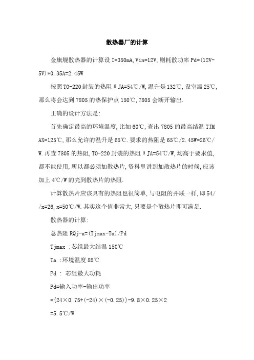
散热器厂的计算金旗舰散热器的计算设I=350mA,Vin=12V,则耗散功率Pd=(12V-5V)*0.35A=2.45W按照TO-220封装的热阻θJA=54℃/W,温升是132℃,设室温25℃,那么将会达到7805的热保护点150℃,7805会断开输出.正确的设计方法是:首先确定最高的环境温度,比如60℃,查出7805的最高结温TJM AX=125℃,那么允许的温升是65℃.要求的热阻是65℃/2.45W=26℃/ W.再查7805的热阻,TO-220封装的热阻θJA=54℃/W,均高于要求值,都不能使用,所以都必须加散热片,资料里讲到加散热片的时候,应该加上4℃/W的壳到散热片的热阻.计算散热片应该具有的热阻也很简单,与电阻的并联一样,即54/ /x=26,x=50℃/W.其实这个值非常大,只要是个散热片即可满足.散热器的计算:总热阻RQj-a=(Tjmax-Ta)/PdTjmax :芯组最大结温150℃Ta :环境温度85℃Pd : 芯组最大功耗Pd=输入功率-输出功率={24×0.75+(-24)×(-0.25)}-9.8×0.25×2=5.5℃/W总热阻由两部分构成,其一是管芯到环境的热阻RQj-a,其中包括结壳热阻RQj-C和管壳到环境的热阻RQC-a.其二是散热器热阻RQd-a,两者并联构成总热阻.管芯到环境的热阻经查手册知 RQj-C=1.0 R QC-a=36 那么散热器热阻RQd-a应<6.4. 散热器热阻RQd-a=[(10/kd) 1/2+650/A]C其中k:导热率铝为2.08d:散热器厚度cmA:散热器面积cm2C:修正因子取1按现有散热器考虑,d=1.0 A=17.6×7+17.6×1×13算得散热器热阻RQd-a=4.1℃/W,散热器选择及散热计算目前的电子产品主要采用贴片式封装器件,但大功率器件及一些功率模块仍然有不少用穿孔式封装,这主要是可方便地安装在散热器上,便于散热。
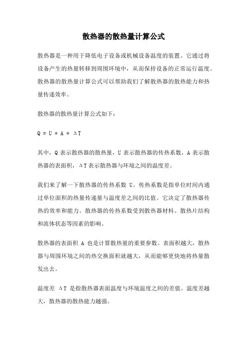
散热器的散热量计算公式散热器是一种用于降低电子设备或机械设备温度的装置。
它通过将设备产生的热量转移到周围环境中,从而保持设备的正常运行温度。
散热器的散热量计算公式可以帮助我们了解散热器的散热能力和热量传递效率。
散热器的散热量计算公式如下:Q = U * A * ΔT其中,Q表示散热器的散热量,U表示散热器的传热系数,A表示散热器的表面积,ΔT表示散热器与环境之间的温度差。
我们来了解一下散热器的传热系数U。
传热系数是指单位时间内通过单位面积的热量传递量与温度差之间的比值。
它决定了散热器传热的效率和能力。
散热器的传热系数受到散热器材料、散热片结构和流体状态等因素的影响。
散热器的表面积A也是计算散热量的重要参数。
表面积越大,散热器与周围环境之间的热交换面积就越大,从而能够更快地将热量散发出去。
温度差ΔT是指散热器表面温度与环境温度之间的差值。
温度差越大,散热器的散热能力越强。
散热器的散热量计算公式可以帮助我们评估散热器的散热性能。
通过调整散热器材料、改进散热片结构和优化流体状态,可以提高散热器的传热系数和表面积,从而提高散热器的散热能力。
除了散热器自身的设计和性能,散热器的散热量还受到其他因素的影响。
例如,周围环境的温度和湿度、设备的功率和工作状态等都会对散热器的散热效果产生影响。
在实际应用中,我们可以根据设备的功率、工作温度和环境温度等参数,计算出散热器所需的散热量。
然后,根据散热器的传热系数和表面积,选择合适的散热器型号和规格。
散热器的散热量计算公式是评估散热器散热性能的重要工具。
通过合理选择散热器和优化散热系统设计,可以有效降低设备温度,提高设备的可靠性和稳定性。
在未来的发展中,我们可以期待散热器技术的进一步创新和提高,以满足不断增长的散热需求。
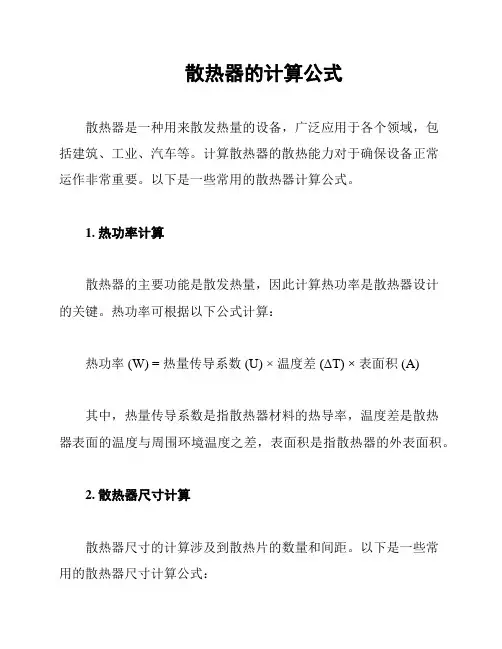
散热器的计算公式
散热器是一种用来散发热量的设备,广泛应用于各个领域,包
括建筑、工业、汽车等。
计算散热器的散热能力对于确保设备正常
运作非常重要。
以下是一些常用的散热器计算公式。
1. 热功率计算
散热器的主要功能是散发热量,因此计算热功率是散热器设计
的关键。
热功率可根据以下公式计算:
热功率 (W) = 热量传导系数 (U) ×温度差(ΔT) × 表面积 (A)
其中,热量传导系数是指散热器材料的热导率,温度差是散热
器表面的温度与周围环境温度之差,表面积是指散热器的外表面积。
2. 散热器尺寸计算
散热器尺寸的计算涉及到散热片的数量和间距。
以下是一些常
用的散热器尺寸计算公式:
- 散热片数量 (N) = 热功率 (W) / 单个散热片的散热能力 (Q)
其中,单个散热片的散热能力可由散热片的热导率 (K) 和表面积 (A) 计算得出。
- 散热片间距 (D) = 散热器高度 (H) / (散热片数量 (N) - 1)
3. 散热器材料选择
散热器材料的选择是散热器设计中的另一个重要因素。
常用的散热器材料包括铝、铜、不锈钢等。
根据散热需求和成本考虑,选择适当的材料是非常关键的。
4. 其他因素考虑
除了以上的计算公式外,散热器设计还需要考虑其他因素,例如流体流量、风速、散热器的布局等。
这些因素会对散热器的散热能力产生影响,需要进行综合考虑。
综上所述,散热器设计的计算公式涉及热功率、散热器尺寸、材料选择等因素。
根据实际需求合理使用这些公式可以确保散热器的有效运作。
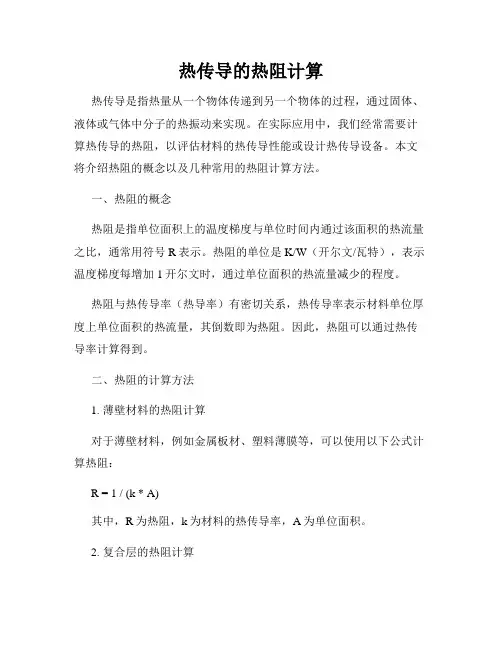
热传导的热阻计算热传导是指热量从一个物体传递到另一个物体的过程,通过固体、液体或气体中分子的热振动来实现。
在实际应用中,我们经常需要计算热传导的热阻,以评估材料的热传导性能或设计热传导设备。
本文将介绍热阻的概念以及几种常用的热阻计算方法。
一、热阻的概念热阻是指单位面积上的温度梯度与单位时间内通过该面积的热流量之比,通常用符号R表示。
热阻的单位是K/W(开尔文/瓦特),表示温度梯度每增加1开尔文时,通过单位面积的热流量减少的程度。
热阻与热传导率(热导率)有密切关系,热传导率表示材料单位厚度上单位面积的热流量,其倒数即为热阻。
因此,热阻可以通过热传导率计算得到。
二、热阻的计算方法1. 薄壁材料的热阻计算对于薄壁材料,例如金属板材、塑料薄膜等,可以使用以下公式计算热阻:R = 1 / (k * A)其中,R为热阻,k为材料的热传导率,A为单位面积。
2. 复合层的热阻计算对于由多层材料组成的复合层结构,可以使用以下公式计算总的热阻:R_total = R_1 + R_2 + R_3 + ... + R_n其中,R_total为总的热阻,R_1、R_2、R_3等分别为每个材料层的热阻。
需要注意的是,计算复合层的热阻时,需要根据不同的传热模式(如平行传热、串联传热等)进行相应的修正。
3. 不均匀材料的热阻计算对于不均匀材料,如中空球、多孔材料等,可以使用以下公式计算热阻:R_total = L / (k_1 * A_1 + k_2 * A_2 + k_3 * A_3 + ... + k_n * A_n)其中,R_total为总的热阻,L为传热长度,k_1、k_2、k_3等为不同材料的热传导率,A_1、A_2、A_3等为不同材料的传热面积。
三、热阻计算的应用热阻计算在工程领域有着广泛的应用,例如在隔热材料的选择中,通过计算不同材料的热阻,可以评估不同材料的隔热效果,选择最适合的材料。
另外,在散热系统的设计中,通过计算散热组件的热阻,可以确定散热器的尺寸和工作参数,以确保系统的稳定性和可靠性。
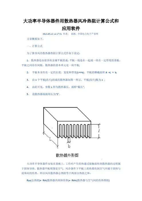
大功率半导体器件用散热器风冷热阻计算公式和应用软件2012-03-12 14:17:31 作者:来源:中国电力电子产业网文章概要如下:一、计算公式为了推导风冷散热器热阻计算公式作如下设定:1,散热器是由很多块金属平板组成,平板一端连在一起成一块有一定厚度的基板,平板之间存在间隙,散热器的基本单元是一块平板;2,平板本身具有一定的长度、宽度和厚度(L×l×b)。
平板的横截面积A =L × b;3,由n个平板(齿片)组成的散热器如图一所示,平板(齿片)数为n ;4,由此可见,参数L即为散热器长,或称“截长”;5,设散热器端面周长为“S”。
大功率半导体器件安装在基板上,工作时产生的热通过接触面传到散热器的过程属于固体导热。
散热器平板周围是空气。
风冷条件下平板上的热要传到空气中属于固体与流体间的传热。
所以风冷散热器总热阻等于两部分热阻之和:Rzo(总热阻)= Rth(散热器内固体传热)+ Rthk(散热器与空气间的传热热阻)引用埃克尔特和..德雷克著的“传热与传质”中的基本原理和公式。
推导出如下实用公式:Ks 为散热器金属材料的导热系数。
20℃时,纯铝:KS = 千卡/ 小时米℃;纯铜:Ks = 332 千卡/ 小时米℃;参数L、l、b、S的单位:米;风速us 单位:米/秒如散热器端面的周边长为S 、散热器的长为L,忽略两端面的面积,散热器的总表面积为: A = S L 。
代入上式后,强迫风冷条件下散热器总热阻公式也可写成:对某一型号的散热器来说参数Ks、b、n、S 都是常数。
用此公式即可求出不同长度L、不同风速us条件下的总热阻,并可作出相应曲线。
本公式的精确性受到多种因素的影响存在一定误差。
主要有:ⅰ,受到环境空气的温度、湿度、气压等自然因素的影响。
如散热器金属的热导系数“Ks”与金属成分及散热器工作时温度有关,本文选用的是20℃时的纯铝。
ⅱ,文中所用的“风速”是指“平均风速”。

大功率半导体器件用散热器风冷热阻计算公式和应用软件-CAL-FENGHAI.-(YICAI)-Company One1大功率半导体器件用散热器风冷热阻计算公式和应用软件2012-03-12 14:17:31作者:来源:中国电力电子产业网文章概要如下:一、计算公式为了推导风冷散热器热阻计算公式作如下设定:1,散热器是由很多块金属平板组成,平板一端连在一起成一块有一定厚度的基板,平板之间存在间隙,散热器的基本单元是一块平板;2,平板本身具有一定的长度、宽度和厚度(L×l×b)。
平板的横截面积A =L × b;3,由n个平板(齿片)组成的散热器如图一所示,平板(齿片)数为n ;4,由此可见,参数L即为散热器长,或称“截长”;5,设散热器端面周长为“S”。
大功率半导体器件安装在基板上,工作时产生的热通过接触面传到散热器的过程属于固体导热。
散热器平板周围是空气。
风冷条件下平板上的热要传到空气中属于固体与流体间的传热。
所以风冷散热器总热阻等于两部分热阻之和:Rzo(总热阻)= Rth(散热器内固体传热)+ Rthk(散热器与空气间的传热热阻)引用埃克尔特和..德雷克着的“传热与传质”中的基本原理和公式。
推导出如下实用公式:Ks 为散热器金属材料的导热系数。
20℃时,纯铝:KS = 千卡/ 小时米℃;纯铜:Ks = 332 千卡/ 小时米℃;参数L、l、b、S的单位:米;风速us 单位:米/秒如散热器端面的周边长为S 、散热器的长为L,忽略两端面的面积,散热器的总表面积为: A = S L 。
代入上式后,强迫风冷条件下散热器总热阻公式也可写成:对某一型号的散热器来说参数 Ks、b、n、S 都是常数。
用此公式即可求出不同长度L、不同风速us条件下的总热阻,并可作出相应曲线。
本公式的精确性受到多种因素的影响存在一定误差。
主要有:ⅰ,受到环境空气的温度、湿度、气压等自然因素的影响。
如散热器金属的热导系数“Ks”与金属成分及散热器工作时温度有关,本文选用的是20℃时的纯铝。
热阻的计算方法首先确定要散热的电子元器件,明确其工作参数,工作条件,尺寸大小,安装方式,选择散热器的底板大小比元器件安装面略大一些即可,因为安装空间的限制,散热器主要依靠与空气对流来散热,超出与元器件接触面的散热器,其散热效果随与元器件距离的增加而递减。
对于单肋散热器,如果所需散热器的宽度在表中空缺,可选择两倍或三倍宽度的散热器截断即可。
关于散热器选择的计算方法参数定义:Rt -------- 总内阻,C /W ;Rtj -------- 半导体器件内热阻,C /W;Rte ------- 半导体器件与散热器界面间的界面热阻,C /W;Rtf -------- 散热器热阻,C /W;Tj --------- 半导体器件结温,C;Te -------- 半导体器件壳温,C;Tf --------- 散热器温度,C;Ta -------- 环境温度,C;Pe -------- 半导体器件使用功率,W ;△Tfa -------- 散热器温升,C;散热计算公式:Rtf =(Tj-Ta) / Pe - Rtj -Rte散热器热阻Rff是选择散热器的主要依据。
Tj和Rtj是半导体器件提供的参数,Pe是设计要求的参数,Rte可从热设计专业书籍中查表。
(1)计算总热阻Rt: Rt= (Tjmax-Ta) / Pe(2)计算散热器热阻Rtf 或温升△ Tfa : Rtf = Rt —Rtj —Rte △ Tfa = Rtf x Pe(3)确定散热器:按照散热器的工作条件(自然冷却或强迫风冷),根据Rtf或厶Tfa和Pe选择散热器,查所选散热器的散热曲线(Rtf曲线或△ Tfa线),曲线上查出的值小于计算值时,就找到了合适的散热器。
对于型材散热器,当无法找到热阻曲线或温升曲线时,可以按以下方法确定:按上述公式求出散热器温升△ Tfa,然后计算散热器的综合换热系数 a :a = 7.2 2 1 2 2 2 3{ W [(Tf-Ta) / 20]} 式中:2 1 ------- 描写散热器L/b对a的影响,(L为散热器的长度,b为两肋片的间距);2 2 ------- 描写散热器h/b对a的影响,(h为散热器肋片的高度);2 3 ------- 描写散热器宽度尺寸W增加时对a的影响;W [(Tf-Ta) /20] -------------- 描写散热器表面最高温度对周围环境的温升对a的影响;以上参数可以查表得到。
![热阻计算[详解]](https://uimg.taocdn.com/80f37cd9db38376baf1ffc4ffe4733687e21fcf8.webp)
热阻计算热阻计算2008-01-13 22:21一般,热阻公式中,Tcmax =Tj - P*Rjc 的公式是在假设散热片足够大而且接触足够良好的情况下才成立的,否则还应该写成Tcmax =Tj - P*(Rjc+Rcs+Rsa)。
Rjc表示芯片内部至外壳的热阻,Rcs表示外壳至散热片的热阻,Rsa表示散热片的热阻。
没有散热片时,Tcmax =Tj - P*(Rjc+Rca)。
Rca表示外壳至空气的热阻。
一般使用条件用Tc =Tj - P*Rjc的公式近似。
厂家规格书一般会给出,Rjc,P等参数。
一般P是在25度时的功耗。
当温度大于25度时,会有一个降额指标。
举个实例:一、三级管2N5551规格书中给出25度(Tc)时的功率是1.5W(P),Rjc是83.3度/W。
此代入公式有:25=Tj-1.5*83.3可以从中推出Tj为150度。
芯片最高温度一般是不变的。
所以有Tc=150-Ptc*83.3,其中Ptc表示温度为Tc时的功耗。
假设管子的功耗为1W,那么,Tc=150-1*83.3=66.7度。
注意,此管子25度(Tc)时的功率是1.5W,如果壳温高于25度,功率就要降额使用。
规格书中给出的降额为12mW/度(0.012W/度)。
我们可以用公式来验证这个结论。
假设温度为Tc,那么,功率降额为0.012*(Tc-25)。
则此时最大总功耗为1.5-0.012*(Tc-25)。
把此时的条件代入公式得出:Tc=150-(1.5-0.012*(Tc-25))×83.3,公式成立。
一般情况下没办法测Tj,可以经过测Tc的方法来估算Ttj。
公式变为:Tj=Tc+P*Rjc同样与2N5551为例。
假设实际使用功率为1.2W,测得壳温为60度,那么:Tj=60+1.2*83.3=159.96此时已经超出了管子的最高结温150度了!按照降额0.012W/度的原则,60度时的降额为(60-25)×0.012=0.42W,1.5-0.42=1.08W。
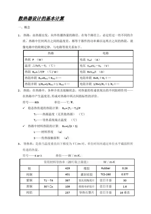
散热器设计的基本计算一、概念1、热路:由热源出发,向外传播热量的路径。
在每个路径上,必定经过一些不同的介质,热路中任何两点之间的温度差,都等于器件的功率乘以这两点之间的热阻,就像电路中的欧姆定律,与电路等效关系如下。
2、热阻:在热路中,各种介质及接触状态,对热量的传递表现出的不同阻碍作用——在热路中产生温度差,形成对热路中两点间指标性的评价。
符号——Rth 单位——℃/W。
✓稳态热传递的热阻计算: R th= (T1-T2)/PT1——热源温度(无其他热源)(℃)T2——导热系统端点温度(℃)✓热路中材料热阻的计算: R th=L/(K·S)L——材料厚度(m)S——传热接触面积(m2)3、导热率:是指当温度垂直向下梯度为1℃/m时,单位时间内通过单位水平截面积所传递的热量。
符号——K or λ单位——W/m-K,二、热设计的目标1、确保任何元器件不超过其最大工作结温(T jmax)✓推荐:器件选型时应达到如下标准民用等级:T jmax≤150℃工业等级:T jmax≤135℃军品等级:T jmax≤125℃航天等级:T jmax≤105℃✓以电路设计提供的,来自于器件手册的参数为设计目标2、温升限值器件、内部环境、外壳:△T≤60℃器件每升高2℃,可靠性下降10%;器件温升为50℃时,寿命只有温升25℃的1/6,电解电容温升超过10℃,寿命下降1/2。
三、计算1、TO220封装+散热器1)结温计算✓热路分析热传递通道:管芯j→功率外壳c→散热器s→环境空气a注:因Rth ca较大,忽略不影响计算,故可省略。
Rth ja≈Rth jc+Rth cs+Rth sa≈(T结温-T环温)/P✓条件Rth jc——器件手册查询Rth cs——材料热阻:R th绝缘垫=L绝缘垫厚度/(K绝缘垫·S绝缘垫接触c的面积)Rth sa——散热器热阻曲线图查询T结温——器件手册查询(待计算数值)T环温——任务指标中的工作环境要求P ——电路设计计算✓计算T结温=(Rth jc+Rth cs+Rth sa)·P+T环温<手册推荐结温✓注:注意单位统一;判定结温温升限值是否符合。

对流散热的热阻计算方法
对流散热的热阻计算方法
对流散热是通过流体(通常是空气)与物体表面之间的传热方式。
对于计算对流散热的热阻,可以按照以下步骤进行:
第一步:确定传热表面的几何形状和尺寸。
传热表面的几何形状和尺寸将直接影响对流散热的强度。
例如,一个平板的散热强度与其表面积成正比。
第二步:确定传热流体的性质和流速。
对流散热的强度还取决于传热流体的性质和流速。
通常使用的传热流体是空气,其性质可通过温度、压力和湿度等参数来确定。
第三步:确定对流传热系数。
对流传热系数描述了流体对物体传热的能力。
它是一个经验值,可通过实验或文献资料获取。
对于一般情况下的自然对流散热,可以使用Grashof数和Prandtl数来估计对流传热系数。
第四步:计算对流散热的热阻。
对流散热的热阻表示传热表面与环境之间的温度差与散热功率之间的比值。
热阻可以通过以下公式计算:
热阻 = 温度差 / 散热功率
其中,温度差是传热表面的温度与环境温度之差,散热功率是传热表面从物体中散失的热量。
第五步:考虑复杂情况。
在实际应用中,对流散热可能会受到其他因素的影响,如风速、相对湿度等。
如果需要考虑这些因素,可以使用更复杂的计算方法,如计算流体力学(CFD)模拟或经验公式。
综上所述,计算对流散热的热阻需要确定传热表面的几何形状和尺寸,传热流体的性质和流速,以及对流传热系数。
通过计算热阻,可以评估对流散热的强度,并为热设计和散热系统的选择提供依据。
散热片热阻计算散热片热阻是指散热片在散热过程中阻碍热量传递的程度。
散热片是一种用于散热的设备,通常由金属制成,具有较好的导热性能。
在电子设备、汽车发动机、空调等各种应用中,散热片起着重要的散热作用。
散热片的热阻是指单位面积上热量通过散热片的难度,其计算公式为:热阻 = 温度差 / 热流率热阻越小,热量传递越顺畅,散热效果越好。
散热片的热阻主要由以下几个因素决定:1. 散热片材料的导热性能:散热片通常采用导热性能较好的金属材料,如铝、铜等。
这些金属具有较高的热导率,能够快速传导热量,从而降低热阻。
2. 散热片的结构形式:散热片的结构形式也会影响其热阻。
散热片通常采用片状或翅片状的结构,增加了散热面积,提高了热量的散发能力。
同时,翅片的设计也会影响热阻的大小,合理的翅片结构能够增加热量的传导效率。
3. 散热片与散热介质之间的接触热阻:散热片通常需要与散热介质(如风扇、散热鳍片等)接触,将热量传递给散热介质。
接触热阻取决于接触面的平整度、接触面积、接触介质的导热性能等因素。
为了减小接触热阻,通常需要采取一些措施,如增加接触面积、使用导热硅脂等。
4. 散热片的尺寸和形状:散热片的尺寸和形状也会影响热阻。
一般来说,散热片的尺寸越大,散热面积越大,热量传递能力越强,热阻越小。
同时,散热片的形状也会影响热量的传导效率,如翅片的形状和密度等。
在实际应用中,为了降低散热片的热阻,可以采取以下措施:1. 选择导热性能好的材料:选择导热性能好的金属材料,如铝、铜等,能够提高散热片的热传导能力,降低热阻。
2. 设计合理的翅片结构:合理设计翅片的形状和密度,增加散热面积,提高热量的散发能力。
3. 优化散热片与散热介质的接触:采取一些措施,如增加接触面积、使用导热硅脂等,减小散热片与散热介质之间的接触热阻。
4. 增大散热片的尺寸:增大散热片的尺寸,增加散热面积,提高热量的传导效率。
散热片的热阻是影响散热效果的重要指标。
通过选择合适的材料、合理设计翅片结构、优化散热片与散热介质的接触方式以及增大散热片的尺寸等措施,可以有效降低散热片的热阻,提高散热效果,确保设备的正常运行和稳定性。
热阻的公式热阻这个概念,在物理学中可是相当重要的哟!咱先来说说热阻到底是个啥。
打个比方吧,就像咱们在马路上走路,有时候会遇到一些阻碍,让咱们走得没那么顺畅。
热在传递的过程中也会遇到这样的“阻碍”,这“阻碍”就是热阻。
热阻可以用来衡量热量传递的难易程度。
那热阻的公式是啥呢?热阻(R)等于材料的厚度(d)除以热导率(k)和传热面积(A)的乘积,用公式写出来就是 R = d / (k × A) 。
比如说,有一块厚度为 10 厘米的木板,热导率是 0.1 瓦/(米·开尔文),传热面积是 1 平方米。
那按照公式来算,热阻 R = 0.1 米 /(0.1×1) = 1 开尔文/瓦。
这就意味着,要让 1 瓦的热量通过这块木板,会产生 1 开尔文的温差。
我记得有一次,我在给学生们讲解热阻这个知识点的时候,发生了一件特别有意思的事儿。
当时我拿了两块材质不同、厚度相同的板子,一块是木板,一块是铝板。
我在板子的一边加热,然后让同学们用手去感受另一边的温度变化。
同学们都特别好奇,一个个瞪大眼睛,伸着小手去感受。
结果发现铝板那一边很快就热了,而木板那一边温度变化很小。
这时候我就趁机跟他们说:“同学们,这就是因为木板的热阻大,铝板的热阻小呀,热量在铝板里传递就容易得多,在木板里就困难一些。
”同学们恍然大悟,那场面,可有趣啦!再深入讲讲热阻这个公式哈。
其中的热导率(k),它反映了材料本身导热的能力。
像金属的热导率一般就比较高,比如铜、铝这些,所以它们常常被用来制作散热器,能快速把热量散出去。
而像木头、塑料这些材料,热导率就低,热阻就大。
厚度(d)就很好理解啦,材料越厚,热量要穿过它就越难,热阻也就越大。
传热面积(A)也会影响热阻哦。
如果传热面积大,热量传递就相对容易些,热阻就会小一点。
在实际生活中,热阻的概念用处可大了。
比如说咱们家里的暖气,管道和暖气片的材质选择、厚度设计,都得考虑热阻,这样才能保证咱们的屋子能暖暖和和的。
热阻的计算公式和含义
热阻是指导热传递能力的指标,表示物体和材料对热传导的反应
能力,通常用符号R表示,单位是K/W。
在工程应用中,热阻的概念非常重要,它在热管理方面起到了关键性的作用。
热阻的计算公式是R = ΔT / Q,其中ΔT 表示物体两端温度差,Q 表示物体所传递的热量。
该公式的意义是,热阻是物体两端温度差
与热流的比值。
热阻越小,则热传导的能力越强,反之则越弱。
因此,热阻越小的材料越适合用于热传导的应用中。
举个例子来说,假设我们要设计一种散热器,用来降低某个电子
元件的温度。
我们需要选择一种能够提供良好热传导的材料,这个材
料需要具有低的热阻。
当热阻越小,热阻值就越接近于零,因此在相
同的温度差下,热传导能力就会更强。
热阻的单位K/W,其实是由温度单位K和功率单位W组成的。
可以通过改变这两个单位之间的换算比例来改变热阻的大小。
例如,如果
我们把温度单位从K修改为C,那么相应的热阻值就需要乘以1.8。
这
种单位的选择取决于具体的应用场景和需要精度的程度。
总之,热阻在工程应用中扮演着关键角色。
掌握热阻的概念和计
算方法,可以帮助我们更好地设计和选择适合的热传导材料,从而优
化热管理系统,提高热传导效率。
热阻与传热系数关系公式在我们的日常生活和各种工程应用中,热阻与传热系数这两个概念可是相当重要的呢。
先来说说热阻,简单来讲,热阻就像是一条道路上的阻碍,会让热量的传递不那么顺畅。
想象一下,冬天的时候,你穿着厚厚的羽绒服,这羽绒服就相当于给热量的传递增加了热阻,让你的身体热量不容易散失出去,从而让你感到温暖。
而传热系数呢,则是衡量热量传递快慢的一个指标。
传热系数越大,热量传递得就越快。
比如说,金属的传热系数通常比塑料大得多,所以用金属锅做饭,热量能很快传递给食物,煮东西就快。
那热阻和传热系数之间到底有啥关系呢?其实啊,它们俩就像是一对欢喜冤家。
热阻越大,传热系数就越小;反过来,热阻越小,传热系数就越大。
这就好比在一条路上,障碍物越多(热阻大),车跑得就越慢(传热效率低,传热系数小);障碍物越少(热阻小),车就能跑得更快(传热效率高,传热系数大)。
我记得有一次,家里的空调出了点小毛病。
大夏天的,热得不行。
维修师傅来检查的时候就提到了热阻和传热系数的问题。
他说空调里的某些部件因为老化,热阻增大了,导致传热系数下降,制冷效果就变差了。
咱们再深入一点说,热阻和传热系数的关系公式可以表示为:传热系数 = 1 / 热阻。
这个公式就像一把钥匙,能帮我们解开很多与热传递相关的谜题。
比如说,在设计一个散热器的时候,如果我们想要让它的散热效果好,也就是传热系数大,那就要想办法减小热阻。
这可能意味着要选择导热性能好的材料,优化散热器的结构,增加散热面积等等。
在工业生产中,对热阻和传热系数的准确把握更是至关重要。
比如在制造发动机的时候,要考虑如何让发动机工作时产生的热量能够快速散发出去,不然发动机温度过高可就容易出故障啦。
这时候,工程师们就得精心计算热阻和传热系数,选择合适的材料和设计方案。
在建筑领域,也离不开对热阻和传热系数的考量。
冬天要保暖,就得增加墙体的热阻,减少热量向外散失;夏天要隔热,也得通过合理的设计来控制热传递。
散热器的扩散热阻计算
1、什么是扩散热阻?
当热源与底板的面积相差比较大时,热量从热源中心往边缘扩散所形成热阻叫扩散热阻。
图1扩散热阻示意
2、如何计算?
针对一个底板上贴一个热源的散热状况,如何计算扩散热阻?分两种情况,一个是热源在底板中心,另一个是不在中心。
针对第一种情况的扩散热阻计算如下:
As:热源面积
Ap:底板面积
t:底板厚度
R0:散热器的平均热阻(从地板厚度的一半之处到环境的热阻)k:散热器材料的导热系数
假设其他参数已知,扩散热阻Rc的计算公式如下:
其中,系数λ是一个由Ap和As计算出来的因子。
从上可以看出,总热阻为扩散热阻与散热器的平均热阻的总和。
针对热源不在中心的情况,需要对公示1进行修正。
增加修正系数C:
而C的计算如下:
假设一个正方形的底板,热源也是正方形,由于对称的关系,取四分之一底板来做分析:
图2:2种热源不在中心的状况
如图2所示,左侧的图,热源的坐标为(x,0),右侧的图中热源坐标为(x,x)。
左侧图中的C=1.414(根号2)。
右侧的C=2 ,如何推算需另外讨论。
如图2中的2种热源位置,热源的大小为25*25mm的话,最大的扩散热阻分别计算如下:
总热阻分别为2.259℃/W和3.334℃/W。
对于上述两种状况,平均热阻R0是不变的,即平均热阻与热源的位置无关。
散热器扩散热阻的计算Accident?Consider the scenario where a designer wishes to incorporate a newly developed device into a system and soon learns that a heat sink is needed to cool the device. The designer finds a rather large heat sink in a catalog which marginally satisfies the required thermal criteria. Due to other considerations, such as fan noise and cost constraints, an attempt to use a smaller heat sink proved futile, and so the larger heat sink was accepted into the design. A prototype was made which, unfortunately, burned-out during the initial validation test, the product missed the narrow introduction time, and the project was canceled. What went wrong?The reasons could have been multi-fold. But, under this scenario, the main culprit could have been the spreading resistance that was overlooked during the design process. It is very important for heat sink users to realize that, unless the heat sink is custom developed for a specific application, thermal performance values provided in vendor's catalogs rarely account for the additional resistances coming from the size and location considerations of a heat source. It is understandable that the vendors themselves could not possibly know what kind of devices the users will be cooling with their products.Figure 1 - Normalized local temperature rise with heat sources of different size; from L to R, source area =100%, 56%, 25%, 6%, of heat-sink areaIntroductionSpreading or constriction resistances exist whenever heat flows from one region to another in different cross sectional area. In the case of heat sink applications, the spreading resistance occurs in the base-plate when a heat source of a smaller footprin footprint area is mounted on a heat sink with a larger base-plate area. This results in a higher local temperature at the location where the heat source is placed. Figure 1 illustrates how the surface temperature of a heat sink base-plate would respond as the size of the heat source is progressively reduced from left to right with all other conditions unchanged: the smaller the heat source, the more spreading has to take place, resulting in a greater temperature rise at the center. In this example, the effect of the edge surfaces of the heat sink is ignored and the heat source is assumed to be generating uniform heat flux. In cases where the footprint of a heat sink need not be much larger than the size of the heat source, the contribution of the spreading resistance to the overall device temperaturerise may be insignificant and usually falls within the design margin. However, in an attempt to remove more heat from today's high performance devices, a larger heat sink is often used and, consequently, the impact of spreading resistance on the performance of a heat sink is becoming an important factor that must not be ignored in the design process. It is not uncommon to find in many high performance, high power applications that more than half the total temperature rise of a heat sink is attributed to the spreading resistance in the base-plate.The objectives of this article are:1) to understand the physics and parameters associated with spreading resistance2) to provide a simple design correlation for accurate prediction of the resistance3) to discuss and clarify the concept of spreading resistance with an emphasis on the practical use of the correlation in heat sink applicationsThe correlation provided herein was originally developed in references 1 and 2. This article is an extension of the earlier presentation.Spreading ResistanceBefore we proceed with the analysis, let us attend to what the temperature distributions shown in Fig. 1 are telling us. The first obvious one, as noted earlier, is that the maximum temperature at the center increases as the heat source becomes smaller. Another important observation is that, as the temperature rises in the center, the temperatures along the edges of the heat sink decrease simultaneously. It can be shown that this happens in such a way that the area-averaged surface temperature of the heat sink base-plate has remained the same. In other words, the average heat sink thermal performance is independent of the size of a heat source. In fact, as will be seen later, it is also independent of the location of the heat source.The spreading resistance can be determined from the following set of parameters: ∙footprint or contact area of the heat source, A s∙footprint area of the heat sink base-plate, A p∙thickness of the heat sink base-plate, t∙thermal conductivity of the heat sink base-plate, k∙average heat sink thermal resistance, R0We will assume, for the time being, that the heat source is centrally mounted on the base-plate, and the heat sink is cooled uniformly over the exposed finned surface. These two assumptions will be examined in further detail. Figure 2 shows a two-dimensional side view of the heat sink with heat-flow lines schematically drawn in the base-plate whose thickness is greatly exaggerated. At the top, the corresponding surface temperature variation across the center line of the base-plate is shown by the solid line. The dotted line represents the average temperature of the surface which is, again, independent of theheat source size and can be easily determined by multiplying R0 with the total amount of heat dissipation, denoted as Q.As indicated in Fig. 2, the maximum constriction resistance R c, which accounts for the local temperature rise over the average surface temperature, is the only additional quantity that is needed for determining the maximum heat sink temperature. It can be accurately determined from the following correlation.Figure 2 - Two dimensional schematic view of local resistance or temperature variation of a heat sinkshown with heat flow LinesNote that the correlation addresses neither the shape of the heat source nor that of the heat sink base-plate. It was found in the earlier study that this correlation typically results in an accuracy of approximately 5% over a wide range of applications with many combinations of different source/sink shapes, provided that the aspect ratio of the shapes involved does not exceed 2.5. See references 1 and 2 for further discussions.Example ProblemConsider an aluminum heat sink (k = 200W/mK) with base-plate dimensions of 100 x 100 x 1.3 mm thick. According to the catalog, the thermal resistance of this heat sink under a given set of conditions is 1.0 °C/W. Find the maximum resistance of the heat sink if used to cool a 25 x 25 mm device.SolutionsWith no other specific descriptions, it is assumed that the heat source is centrally mounted, and the given thermal resistance of 1.0 °C/W represents the average heat sink performance. From the problem statement, we summarize:∙A s = 0.025 x 0.025 = 0.000625 m2∙A p = 0.1 x 0.1 = 0.01 m2∙t = 0.0013 m∙k = 200 W/mK∙R0 = 1.0 °C/WTherefore,Hence, the maximum resistance, R total , is:R total = R o + R c = 1.0 + 0.66 = 1.66 °C/WReaders should note the far right temperature distribution in Fig. 1 which is the result of a numerical simulation for the present problem in rectangular coordinates.Effect of Source LocationIn the following two sections, we will limit our examination to the current example problem. As we shall see, the result of this limited case study will allow us to draw some general yet useful conclusions. Suppose the same heat source in the above example was not centrally located, but mounted a distance away from the center. Obviously, the maximum temperature would further rise as compared to that found in the above example. Figure 3 shows the local resistances corresponding to two such cases:Figure 3 - Heat-sink local resistance showing the effect of source location:from L to R, heat source at (37.5,0) and (37.5,37.5)the first one is for the case where the heat source is mounted midway along the edge, and the other, where it is mounted on one corner of the heat sink. For these two special cases,the maximum spreading resistance can be calculated by using Eq. (1) for R c with input parameters t and R0 modified as shown below:R c = C x R c (A p,A s,k,t/C,R0/C)(3) with for the first case, and C = 2 for the second case. It is to be noted that this expression is independent of the source size. Numerically, for the current problem with a 25 x 25 mm heat source, it results in the maximum spreading resistances of 1.29 and2.38 °C/W, or the total resistances of 2.29 and3.38 °C/W for the first and second cases, respectively. For both cases, it can be shown that the average surface resistance has not changed from unity.For other intermediate source locations, numerical simulations were carried out and a plot is provided in Fig. 4 for the correction factor C f which can be used to compute the total resistance asR total = R0 + C f R c(4) where R c is determined from Eq. (1), given for the case with the heat source placed at the center.Figure 4 - Correction factor as a function of source locationThe coordinates in Fig. 4 indicate the location of the center of the heat source measured from the center of the base-plate in mm: the case with a centrally located heat source corresponds to (0,0), and the cases shown in Fig. 3 correspond to (37.5,0) and (37.5,37.5) for the first and second cases, respectively. Only one quadrant is shown in Fig. 4 as they would be, owing to the assumption of uniform cooling, symmetrical about (0,0). As can be seen from the figure, the correction factor increases from 1 as the heat source is placed away from the center. It is worthwhile noting that the increase is, however, very minimal over a wide region near the center, and most increases occur closer to the edges.Unlike C in the earlier expression, C f is case dependent (i.e. it depends on the heat-source size). However, it was found that the plots of C f obtained for many other cases exhibit essentially the same profile as that shown in Fig. 4, with magnitudes at the corners determined from Eq. (3), and the domain of the plot defined by the maximum displacement of the heat source. Based on this observation, a general conclusion can be made: for all practical purposes, as long as the heat source is placed closer to the center than to the edges of the heat sink, the correctional increase in the spreading resistance may be ignored, and C f =1 may be used. As noted above, this would introduce a small error of no greater than 5-10% in the spreading resistance which, in turn, is a fraction of the total resistance.So far, we have assumed a uniform cooling over the entire finned-surface area of the base-plate. Although this is a useful assumption, it is seldom realized in actual situations. It is well known that, due to the thinner boundary layer and the less down-stream heating effect, a device would be cooled more effectively if it is mounted toward the air inlet side. Again, a numerical simulation is carried out using our example problem with the boundary layer effect included.Figure 5 shows the resulting modified correction factor as a function of the distance from the center of the heat sink to the heat source placed along the center line at y=0: x = -37.5 mm corresponds to the front most leading edge location of the heat source and x = 37.5 mm the rear most trailing edge placement.Figure 5 - Correction factor modified for boundary layer effect at y=0As can be seen from the figure, it is possible to realize a small improvement by placing the heat source forward of the center location where C f < 1. However, it was experienced in practice that accommodating a heat source away from the center and ensuring its mounting orientation often cause additional problems during manufacturing and assembly processes.Summary and DiscussionA simple correlation equation is presented for determining spreading resistances in heat sink applications. A sample calculation is carried out for a case with a heat source placed at the center of the heat sink base-plate and a means to estimate the correction factor to account for the effect of changing the heat-source location is provided. It is to be noted that the correlation provided herein is a general solution which reduces to the well known Kennedy's solution3 when R0 approaches 0: the mathematical equivalent of isothermal boundary condition. Kennedy's solution is valid only when R0 is sufficiently small such that the fin-side of the heat sink base-plate is close to isothermal. Otherwise, Kennedy's solution, representing the lower boundary of the spreading resistance, may result in gross underestimation of the resistance.The earlier study revealed that, depending on the relative magnitude of the average heat sink resistance, the spreading resistance may either increase or decrease with the base-plate thickness. If the heat sink resistance is sufficiently small, as in liquid cooled heat sink applications, the spreading resistance always increases with the thickness, and an optimum thickness does not exist. On the other hand, if the heat sink resistance is large, as experienced in most air-cooled applications, the spreading resistance decreases with the thickness and a finite optimum thickness exists.It is to be noted that the present correlation calculates the spreading resistance only in the base-plate and does not account for the effect of additional spreading that may exist in other places, such as the fins in a planar heat sink. This additional spreading in the fins usually affects the spreading resistance in a similar way to a thicker base-plate. The current author found that an increase of 20% in the base-plate thickness during the calculation roughly accounts for the effect of this additional spreading in the fins of the same material for most planar heat sinks under air cooling. No modification is required for pin-fin heat sinks.Seri LeeAmkor Electronics, Inc.1900 South Price RoadChandler, AZ 85248, USATel: +1 (602) 821-2408 x 5459Fax: +1 (602) 821-6730Email: lees@References1.S. Lee, S. Song, V. Au, and K.P. Moran, Constriction/Spreading Resistance Model for ElectronicPackaging, Proceedings of the 4th ASME/JSME Thermal Engineering Joint Conference, Vol. 4, 1995, pp. 199-206.2.S. Song, S. Lee, and V. Au, Closed Form Equation for Thermal Constriction/Spreading Resistanceswith Variable Resistance Boundary Condition, Proceedings of the 1994 IEPS Conference, 1994, pp.111-121.3. D. P. Kennedy, Spreading Resistance in Cylindrical Semiconductor Devices, Journal of AppliedPhysics, Vol. 31, 1960, pp. 1490-1497.。