北京大学ACM暑期课讲义-lcc-数论

数论专题讲义数论专题数论主要分为以下几个模块：1、数的整除问题2、质数合数与分解质因数3、约数与倍数4、余数问题5、奇数与偶数6、位值原理7、完全平方数8、数字谜问题一、分裂问题一.一个数的末位能被2或5整除，这个数就能被2或5整除；一个数的末两位能被4或25整除，这个数就能被4或25整除；一个数的末三位能被8或125整除，这个数就能被8或125整除；2.一个位数数字和能被3整除，这个数就能被3整除；一个数各位数数字和能被9整除，这个数就能被9整除；3.如果一个整数的奇数位数和偶数位数之和的差可以除以11，那么这个数可以除以114.如果一个整数的末三位与末三位以前的数字组成的数之差能被7、11或13整除，然后这个数字可以除以7、11或13【备注】（以上规律仅在十进制数中成立.）性质1如果数a和数b都能被数c整除，那么它们的和或差也能被c整除．即如果ca，CB，然后是C（a±b）性质2如果数a能被数b整除，b又能被数c整除，那么a也能被c整除．即如果boa，Cob，然后COA用同样的方法，我们还可以得出：属性3如果a可以被B和C的乘积除，那么a也可以被B和C除。

也就是说，如果bcoa，那么么boa，coa．属性4如果数字a可以被数字B或数字C除，并且数字B和数字C是互质的，那么a必须被数字B除1/10除以和C的乘积。

也就是说，如果boa，COA和（B，C）=1，那么bcoa性质5如果数a能被数b整除，那么am也能被bm整除．如果b｜a，那么bm｜am（m是非零整数）；性质6如果数a能整除数b，且数c能被数d整除，那么ac也能整除bd，如果b｜a，和D C，然后是BD AC；1、整除判定特征如果六位数的数字是1992□ □ 可以除以105，最后两位数是多少？2、数的整除性质应用如果15abc6可以除以36，商是最小的，那么a、B和C分别是什么？3、整除综合性问题已知：23！？258d20c6738849766ab000。

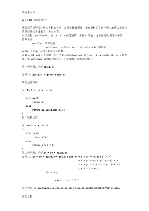
poj 1061 青蛙的约会这题用的是解线性同余方程的方法，之前没接触到过，搜索资料后看到一个人的博客里面讲的很好就拷贝过来了。

内容如下：对于方程：ax≡b(mod m)，a，b，m都是整数，求解x 的值，这个就是线性同余方程。

符号说明：mod表示：取模运算ax≡b(mod m)表示：(ax - b) mod m = 0，即同余gcd(a,b)表示：a和b的最大公约数求解ax≡b(mod n)的原理：对于方程ax≡b(mod n)，存在ax + by = gcd(a,b)，x，y是整数。

而ax≡b(mod n)的解可以由x，y来堆砌。

具体做法如下：第一个问题：求解gcd(a,b)定理一：gcd(a,b) = gcd(b,a mod b)欧几里德算法int Euclid(int a,int b){if(b == 0)return a;elsereturn Euclid(b,mod(a,b));}附：取模运算int mod(int a,int b){if(a >= 0)return a % b;elsereturn a % b + b;}第二个问题：求解ax + by = gcd(a,b)定理二：ax + by = gcd(a,b)= gcd(b,a mod b) = b * x' + (a mod b) * y'= b * x' + (a - a / b * b) * y'= a * y' + b * (x' - a / b * y')= a * x + b * y则：x = y'y = x' - a / b * y'以上内容转自/redcastle/blog/item/934b232dbc40d336349bf7e4.html由这个可以得出扩展的欧几里德算法：int exGcd(int a, int b, int &x, int &y) {if(b == 0){x = 1;y = 0;return a;}int r = exGcd(b, a % b, x, y);int t = x;x = y;y = t - a / b * y;return r;}代码：#include<iostream>#include<cstdlib>#include<cstring>#include<cmath>using namespace std;__int64 mm,nn,xx,yy,l;__int64 c,d,x,y;__int64 modd(__int64 a, __int64 b){if(a>=0)return a%b;elsereturn a%b+b;}__int64 exGcd(__int64 a, __int64 b) {if(b==0){x=1;y=0;return a;}__int64 r=exGcd(b, a%b);__int64 t=x;x=y;y=t-a/b*y;return r;}int main(){scanf("%I64d %I64d %I64d %I64d %I64d",&xx,&yy,&mm,&nn,&l);if(mm>nn) //分情况{d=exGcd(mm-nn,l);c=yy-xx;}else{d=exGcd(nn-mm,l);c=xx-yy;}if(c%d != 0){printf("Impossible\n");return 0;}l=l/d;x=modd(x*c/d,l); ///取模函数要注意printf("%I64d\n",x);system("pause");return 0;}POJ 1142 SmithNumber题意：寻找最接近而且大于给定的数字的SmithNumber什么是SmithNumber？用sum(int)表示一个int的各位的和，那一个数i如果是SmithNumber,则sum（i） =sigma( sum(Pj )),Pj表示i的第j个质因数。

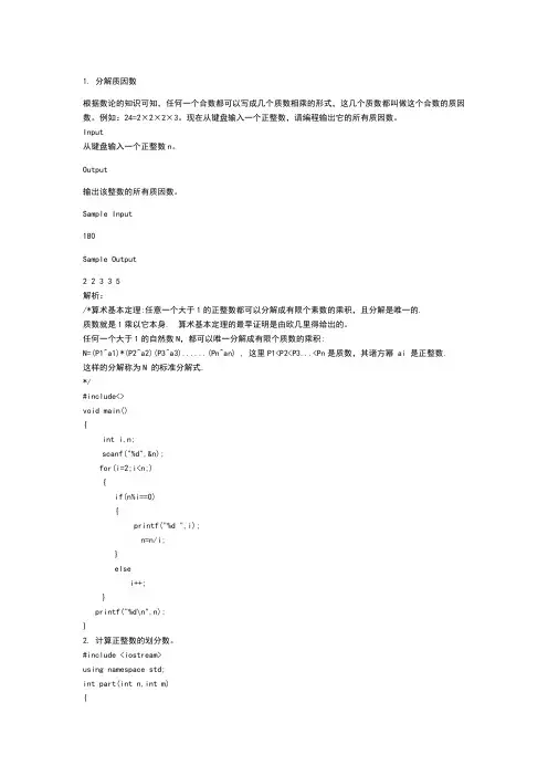
1. 分解质因数根据数论的知识可知，任何一个合数都可以写成几个质数相乘的形式，这几个质数都叫做这个合数的质因数。

例如：24=2×2×2×3。

现在从键盘输入一个正整数，请编程输出它的所有质因数。

Input从键盘输入一个正整数n。

Output输出该整数的所有质因数。

Sample Input180Sample Output2 23 3 5解析：/*算术基本定理:任意一个大于1的正整数都可以分解成有限个素数的乘积，且分解是唯一的.质数就是1乘以它本身. 算术基本定理的最早证明是由欧几里得给出的。

任何一个大于1的自然数N，都可以唯一分解成有限个质数的乘积:N=(P1^a1)*(P2^a2)(P3^a3)......(Pn^an) , 这里P1<P2<P3...<Pn是质数，其诸方幂 ai 是正整数.这样的分解称为N 的标准分解式.*/#include<>void main(){int i,n;scanf("%d",&n);for(i=2;i<n;){if(n%i==0){printf("%d ",i);n=n/i;}elsei++;}printf("%d\n",n);}2. 计算正整数的划分数。

#include <iostream>using namespace std;int part(int n,int m){if (n<1||m<1)return 0;if (n==1||m==1)return 1;if (n<m)return part(n,n);if (n==m)return part(n,m-1)+1;return part(n,m-1)+part(n-m,m);}void main(){int n,m;cin>>n>>m;cout<<part(n,m)<<endl;}3求一个二位数的13次方后的最后三位数。

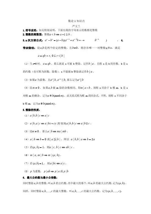
数论 1 知识点严文兰1.符号说明：如无特别说明，下面出现的字母表示的数都是整数2.整数的离散型：整数a <b ⇔a +1 ≤b ，3.n 次方差公式：a n -b n = (a -b)(a n-1 +a n-2b ++b n-1 ) ，4.带余除法：设a, b是两个给定的整数，且b ≠0，则存在唯一一对整数q和r，满足a =qb +r, 0 ≤r <| b |（1）当r=0 时，a =qb ，那么就说a 可被b 整除，记作b | a ，且称a 是b 的倍数，b 是a 的约数（也可称为因数，除数），a 不能被b 整除就记作b /|a ，（2）如果a 为素数，且a n | b, a n+1 /| b, 那么记为a n || b（3）设m ≠ 0 ，如果a, b 被m 除的余数相同，即m | a -b ，则称a 同余于b 模m，b 是a 对模m 的剩余，记为a ≡b(mod m) ，此关系式称为模m 的同余式，不然，则称a 不同余于b 模m，记为a≡/b(mod m)，5.整除的性质：（1）a | b, b| c ⇒a | c（2）a | b, a | c ⇒a | bx +cy ,特别地a | b, b | c ⇒a | b ±c ，（3）设m ≠ 0 ，那么a | b ⇔ma | mb ，（4）a | b ⇒b = 0 或| a |≤| b | ，所以 a | b, b | a ⇒b =±a（5）若(a, b) = 1，则a | c, b | c ⇔ab | c ，（6）m | a, m | b ⇒m | (a, b) ，（7）若(a, b) =1, ，则a | bc ⇔a | c ，（8）p 为素数，p | ab ⇒p | a 或p | b6．最大公约数与最小公倍数：同时整除a, b 的整数，叫a, b 的公约数，其中最大的那个，叫a, b 的最大公约数，记为(a, b) ，同样，同时整除a, b, , c 的最大整数，叫a, b, , c 的最大公约数，记为(a, b, , c) ，1 2 1 2同样，同时是 a , b ,, c 的倍数的整数，叫 a , b , , c 的公倍数，其中最小的正整数，叫a ,b , ,c 的最小公倍数，记为[a , b , , c ] 。

Class 1: Expectations, variances, and basics of estimationBasics of matrix (1)I. Organizational Matters(1)Course requirements:1)Exercises: There will be seven (7) exercises, the last of which is optional. Eachexercise will be graded on a scale of 0-10. In addition to the graded exercise, ananswer handout will be given to you in lab sections.2)Examination: There will be one in-class, open-book examination.(2)Computer software: StataII. Teaching Strategies(1) Emphasis on conceptual understanding.Yes, we will deal with mathematical formulas, actually a lot of mathematical formulas. But, I do not want you to memorize them. What I hope you will do, is to understand the logic behind the mathematical formulas.(2) Emphasis on hands-on research experience.Yes, we will use computers for most of our work. But I do not want you to become a computer programmer. Many people think they know statistics once they know how to run a statistical package. This is wrong. Doing statistics is more than running computer programs. What I will emphasize is to use computer programs to your advantage in research settings. Computer programs are like automobiles. The best automobile is useless unless someone drives it. You will be the driver of statistical computer programs.(3) Emphasis on student-instructor communication.I happen to believe in students' judgment about their own education. Even though I will be ultimately responsible if the class should not go well, I hope that you will feel part of the class and contribute to the quality of the course. If you have questions, do not hesitate to ask in class. If you have suggestions, please come forward with them. The class is as much yours as mine.Now let us get to the real business.III(1). Expectation and VarianceRandom Variable: A random variable is a variable whose numerical value is determined by the outcome of a random trial.Two properties: random and variable.A random variable assigns numeric values to uncertain outcomes. In a common language, "give a number". For example, income can be a random variable. There are many ways to do it. You can use the actual dollar amounts.In this case, you have a continuous random variable. Or you can use levels of income, such as high, median, and low. In this case, you have an ordinal random variable [1=high,2=median, 3=low]. Or if you are interested in the issue of poverty, you can have a dichotomous variable: 1=in poverty, 0=not in poverty.In sum, the mapping of numeric values to outcomes of events in this way is the essence of a random variable.Probability Distribution: The probability distribution for a discrete random variable X associates with each of the distinct outcomes x i(i = 1, 2,..., k) a probability P(X = x i).Cumulative Probability Distribution: The cumulative probability distribution for a discrete random variable X provides the cumulative probabilities P(X ≤ x) for all values x.Expected Value of Random Variable: The expected value of a discrete random variable X is denoted by E{X} and defined:E{X}=(x i)where: P(x i) denotes P(X = x i). The notation E{ } (read “expectation of”) is called the expectation operator.In common language, expectation is the mean. But the difference is that expectation is a concept for the entire population that you never observe. It is the result of the infinite number of repetitions. For example, if you toss a coin, the proportion of tails should be .5 in the limit. Or the expectation is .5. Most of the times you do not get the exact .5, but a number close to it.Conditional ExpectationIt is the mean of a variable conditional on the value of another random variable.Note the notation: E(Y|X).In 1996, per-capita average wages in three Chinese cities were (in RMB):Shanghai: 3,778Wuhan: 1,709Xi’an: 1,155Variance of Random Variable: The variance of a discrete random variable X is denoted by V{X} and defined:V{X}=i - E{X})2 P(x i)where: P(x i) denotes P(X = x i). The notation V{ }(read “variance of”) is called the variance operator.Since the variance of a random variable X is a weighted average of the squared deviations, (X - E{X})2 , it may be defined equivalently as an expected value: V{X} = E{(X - E{X})2}.An algebraically identical expression is: V{X} = E{X2} - (E{X})2.Standard Deviation of Random Variable: The positive square root of the variance of X is called the standard deviation of X and is denoted by σ{X}:σ{XThe notation σ{ } (read “standard deviation of”) is called the standard deviation operator. Standardized Random Variables: If X is a random variable with expected value E{X} and standard deviation σ{X}, then:Y=}{}{ X XEXσ-is known as the standardized form of random variable X.Covariance: The covariance of two discrete random variables X and Y is denoted by Cov{X,Y} and defined:Cov{X,Ywhere: P(x i, y jThe notation of Cov covariance operator.When X and Y are independent, Cov {X,Y} = 0.Cov {X,Y} = E{(X - E{X})(Y - E{Y})}; Cov {X,Y} = E{XY} - E{X}E{Y}(Variance is a special case of covariance.)Coefficient of Correlation: The coefficient of correlation of two random variables X and Y is denoted by ρ{X,Y} (Greek rho) and defined:where: σ{X} is the standard deviation of X; σ{Y} is the standard deviation of Y; Cov is the covariance of X and Y.Sum and Difference of Two Random Variables: If X and Y are two random variables, then the expected value and the variance of X + Y are as follows:Expected Value: E{X+Y} = E{X} + E{Y};Variance: V{X+Y} = V{X} + V{Y}+ 2 Cov(X,Y).If X and Y are two random variables, then the expected value and the variance of X - Y are as follows:Expected Value: E{X - Y} = E{X} - E{Y};Variance: V{X - Y} = V{X} + V{Y} - 2 Cov(X,Y).Sum of More Than Two Independent Random Variables: If T = X 1 + X 2 + ... + X s is the sumof s independent random variables, then the expected value and the variance of T are as follows:III(2). Properties of Expectations and Covariances:(1) Properties of Expectations under Simple Algebraic Operations)()(x bE a bX a E +=+This says that a linear transformation is retained after taking an expectation.bX a X +=*is called rescaling: a is the location parameter, b is the scale parameter.Special cases are:For a constant: a a E =)(For a different scale: )()(X E b bX E =, e.g., transforming the scale of dollars into the scale of cents.(2) Properties of Variances under Simple Algebraic Operations)()(2X V b bX a V =+This says two things: (1) Adding a constant to a variable does not change the variance of the variable; reason: the definition of variance controls for the mean of the variable[graphics]. (2) Multiplying a constant to a variable changes the variance of the variable by a factor of the constant squared; this is to easy prove, and I will leave it to you. This is the reason why we often use standard deviation instead of variance2x x σσ=is of the same scale as x.(3) Properties of Covariance under Simple Algebraic OperationsCov(a + bX, c + dY) = bd Cov(X,Y).Again, only scale matters, location does not.(4) Properties of Correlation under Simple Algebraic OperationsI will leave this as part of your first exercise:),(),(Y X dY c bX a ρρ=++That is, neither scale nor location affects correlation.IV: Basics of matrix.1. DefinitionsA. MatricesToday, I would like to introduce the basics of matrix algebra. A matrix is a rectangular array of elements arranged in rows and columns:11121211.......m n nm x x x x X x x ⎡⎤⎢⎥⎢⎥=⎢⎥⎢⎥⎣⎦Index: row index, column index.Dimension: number of rows x number of columns (n x m)Elements: are denoted in small letters with subscripts.An example is the spreadsheet that records the grades for your home work in the following way:Name 1st 2nd ....6thA 7 10 (9)B 6 5 (8)... ... ......Z 8 9 (8)This is a matrix.Notation: I will use Capital Letters for Matrices.B. VectorsVectors are special cases of matrices:If the dimension of a matrix is n x 1, it is a column vector:⎥⎥⎥⎥⎦⎤⎢⎢⎢⎢⎣⎡=n x x x x (21)If the dimension is 1 x m, it is a row vector:y' = | 1y 2y .... m y |Notation: small underlined letters for column vectors (in lecture notes)C. TransposeThe transpose of a matrix is another matrix with positions of rows and columns being exchanged symmetrically.For example: if⎥⎥⎥⎥⎦⎤⎢⎢⎢⎢⎣⎡=⨯nm n m m n x x x x x x X 12111211)( (1121112)()1....'...n m n m nm x x x x X x x ⨯⎡⎤⎢⎥⎢⎥=⎢⎥⎢⎥⎣⎦It is easy to see that a row vector and a column vector are transposes of each other. 2. Matrix Addition and SubtractionAdditions and subtraction of two matrices are possible only when the matrices have the same dimension. In this case, addition or subtraction of matrices forms another matrix whoseelements consist of the sum, or difference, of the corresponding elements of the two matrices.⎥⎥⎥⎥⎦⎤⎢⎢⎢⎢⎣⎡±±±±±=Y ±X mn nm n n m m y x y x y x y x y x (11)2121111111 Examples:⎥⎦⎤⎢⎣⎡=A ⨯4321)22(⎥⎦⎤⎢⎣⎡=B ⨯1111)22(⎥⎦⎤⎢⎣⎡=B +A =⨯5432)22(C 3. Matrix MultiplicationA. Multiplication of a scalar and a matrixMultiplying a scalar to a matrix is equivalent to multiplying the scalar to each of the elements of the matrix.11121211Χ...m n nm cx c cx cx ⎢⎥⎢⎥=⎢⎥⎢⎥⎣⎦ B. Multiplication of a Matrix by a Matrix (Inner Product)The inner product of matrix X (a x b) and matrix Y (c x d) exists if b is equal to c. The inner product is a new matrix with the dimension (a x d). The element of the new matrix Z is:c∑=kj ik ijy x zk=1Note that XY and YX are very different. Very often, only one of the inner products (XY and YX) exists.Example:⎥⎦⎤⎢⎣⎡=4321)22(x A⎥⎦⎤⎢⎣⎡=10)12(x BBA does not exist. AB has the dimension 2x1⎥⎦⎤⎢⎣⎡=42ABOther examples:If )53(x A , )35(x B , what is the dimension of AB? (3x3)If )53(x A , )35(x B , what is the dimension of BA? (5x5)If )51(x A , )15(x B , what is the dimension of AB? (1x1, scalar)If )53(x A , )15(x B , what is the dimension of BA? (nonexistent)4. Special MatricesA. Square Matrix)(n n A ⨯B. Symmetric MatrixA special case of square matrix.For )(n n A ⨯, ji ij a a =. All i, j .A' = AC. Diagonal MatrixA special case of symmetric matrix⎥⎥⎥⎥⎦⎢⎢⎢⎢⎣=X nn x x 0 (2211)D. Scalar Matrix0....0c c c c ⎡⎤⎢⎥⎢⎥=I ⎢⎥⎢⎥⎣⎦E. Identity MatrixA special case of scalar matrix⎥⎥⎥⎥⎦⎤⎢⎢⎢⎢⎣⎡=I 10 (101)Important: for r r A ⨯AI = IA = AF. Null (Zero) MatrixAnother special case of scalar matrix⎥⎥⎥⎥⎦⎤⎢⎢⎢⎢⎣⎡=O 00 (000)From A to E or F, cases are nested from being more general towards being more specific.G. Idempotent MatrixLet A be a square symmetric matrix. A is idempotent if....32=A =A =AH. Vectors and Matrices with elements being oneA column vector with all elements being 1,⎥⎥⎥⎥⎦⎤⎢⎢⎢⎢⎣⎡=⨯1......111r A matrix with all elements being 1, ⎥⎥⎥⎥⎦⎤⎢⎢⎢⎢⎣⎡=⨯1...1...111...11rr J Examples let 1 be a vector of n 1's: )1(1⨯n1'1 = )11(⨯n11' = )(n n J ⨯I. Zero VectorA zero vector is⎥⎥⎥⎥⎦⎤⎢⎢⎢⎢⎣⎡=⨯0....001r 5. Rank of a MatrixThe maximum number of linearly independent rows is equal to the maximum number of linearly independent columns. This unique number is defined to be the rank of the matrix. For example,⎥⎥⎥⎦⎤⎢⎢⎢⎣⎡=B 542211014321Because row 3 = row 1 + row 2, the 3rd row is linearly dependent on rows 1 and 2. The maximum number of independent rows is 2. Let us have a new matrix:⎥⎦⎤⎢⎣⎡=B 11014321*学习-----好资料更多精品文档 Singularity: if a square matrix A of dimension ()n n ⨯has rank n, the matrix is nonsingular. If the rank is less than n, the matrix is then singular.。

Class 1: Expectations, variances, and basics of estimationBasics of matrix (1)I. Organizational Matters(1)Course requirements:1)Exercises: There will be seven (7) exercises, the last of which is optional. Eachexercise will be graded on a scale of 0-10. In addition to the graded exercise, ananswer handout will be given to you in lab sections.2)Examination: There will be one in-class, open-book examination.(2)Computer software: StataII. Teaching Strategies(1) Emphasis on conceptual understanding.Yes, we will deal with mathematical formulas, actually a lot of mathematical formulas. But, I do not want you to memorize them. What I hope you will do, is to understand the logic behind the mathematical formulas.(2) Emphasis on hands-on research experience.Yes, we will use computers for most of our work. But I do not want you to become a computer programmer. Many people think they know statistics once they know how to run a statistical package. This is wrong. Doing statistics is more than running computer programs. What I will emphasize is to use computer programs to your advantage in research settings. Computer programs are like automobiles. The best automobile is useless unless someone drives it. You will be the driver of statistical computer programs.(3) Emphasis on student-instructor communication.I happen to believe in students' judgment about their own education. Even though I will be ultimately responsible if the class should not go well, I hope that you will feel part of the class and contribute to the quality of the course. If you have questions, do not hesitate to ask in class. If you have suggestions, please come forward with them. The class is as much yours as mine.Now let us get to the real business.III(1). Expectation and VarianceRandom Variable: A random variable is a variable whose numerical value is determined by the outcome of a random trial.Two properties: random and variable.A random variable assigns numeric values to uncertain outcomes. In a common language, "give a number". For example, income can be a random variable. There are many ways to do it. You can use the actual dollar amounts.In this case, you have a continuous random variable. Or you can use levels of income, such as high, median, and low. In this case, you have an ordinal random variable [1=high,2=median, 3=low]. Or if you are interested in the issue of poverty, you can have a dichotomous variable: 1=in poverty, 0=not in poverty.In sum, the mapping of numeric values to outcomes of events in this way is theessence of a random variable.Probability Distribution: The probability distribution for a discrete random variable Xassociates with each of the distinct outcomes x i (i = 1, 2,..., k ) a probability P (X = x i ). Cumulative Probability Distribution: The cumulative probability distribution for a discreterandom variable X provides the cumulative probabilities P (X ≤ x ) for all values x .Expected Value of Random Variable: The expected value of a discrete random variable X isdenoted by E {X } and defined:E {X } = x i i k=∑1P (x i )where : P (x i ) denotes P (X = x i ). The notation E { } (read “expectation of”) is called theexpectation operator.In common language, expectation is the mean. But the difference is that expectation is a concept for the entire population that you never observe. It is the result of the infinitenumber of repetitions. For example, if you toss a coin, the proportion of tails should be .5 in the limit. Or the expectation is .5. Most of the times you do not get the exact .5, but a number close to it.Conditional ExpectationIt is the mean of a variable conditional on the value of another random variable.Note the notation: E(Y|X).In 1996, per-capita average wages in three Chinese cities were (in RMB):Shanghai: 3,778Wuhan: 1,709Xi ’an: 1,155Variance of Random Variable: The variance of a discrete random variable X is denoted by V {X } and defined:V {X } = i k =∑1(x i - E {X })2 P (x i )where : P (x i ) denotes P (X = x i ). The notation V { } (read “variance of”) is called the variance operator.Since the variance of a random variable X is a weighted average of the squared deviations,(X - E {X })2 , it may be defined equivalently as an expected value: V {X } = E {(X - E {X })2}. An algebraically identical expression is: V {X} = E {X 2} - (E {X })2.Standard Deviation of Random Variable: The positive square root of the variance of X is called the standard deviation of X and is denoted by σ{X }:σ {X } =V X {}The notation σ{ } (read “standard deviation of”) is called the standard deviation operator. Standardized Random Variables: If X is a random variable with expected value E {X } and standard deviation σ{X }, then:Y =}{}{X X E X σ-is known as the standardized form of random variable X .Covariance: The covariance of two discrete random variables X and Y is denoted by Cov {X,Y } and defined:Cov {X, Y } = ({})({})(,)xE X y E Y P x y i j i j j i --∑∑where: P (x i , y j ) denotes P Xx Y y i j (=⋂= ) The notation of Cov { , } (read “covariance of”) is called the covariance operator .When X and Y are independent, Cov {X, Y } = 0.Cov {X, Y } = E {(X - E {X })(Y - E {Y })}; Cov {X, Y } = E {XY } - E {X }E {Y }(Variance is a special case of covariance.)Coefficient of Correlation: The coefficient of correlation of two random variables X and Y isdenoted by ρ{X,Y } (Greek rho) and defined:ρσσ{,}{,}{}{}X Y Cov X Y X Y =where: σ{X } is the standard deviation of X; σ{Y } is the standard deviation of Y; Cov is the covariance of X and Y.Sum and Difference of Two Random Variables: If X and Y are two random variables, then the expected value and the variance of X + Y are as follows:Expected Value : E {X+Y } = E {X } + E {Y };Variance : V {X+Y } = V {X } + V {Y }+ 2 Cov (X,Y ).If X and Y are two random variables, then the expected value and the variance of X - Y are as follows:Expected Value : E {X - Y } = E {X } - E {Y };Variance : V {X - Y } = V {X } + V {Y } - 2 Cov (X,Y ).Sum of More Than Two Independent Random Variables: If T = X 1 + X 2 + ... + X s is the sumof s independent random variables, then the expected value and the variance of T are as follows:Expected Value: E T E X i i s {}{}==∑1; Variance: V T V X i i s {}{}==∑1III(2). Properties of Expectations and Covariances:(1) Properties of Expectations under Simple Algebraic Operations)()(x bE a bX a E +=+This says that a linear transformation is retained after taking an expectation.bX a X +=*is called rescaling: a is the location parameter, b is the scale parameter.Special cases are:For a constant: a a E =)(For a different scale: )()(X E b bX E =, e.g., transforming the scale of dollars into thescale of cents.(2) Properties of Variances under Simple Algebraic Operations)()(2X V b bX a V =+This says two things: (1) Adding a constant to a variable does not change the variance of the variable; reason: the definition of variance controls for the mean of the variable[graphics]. (2) Multiplying a constant to a variable changes the variance of the variable by a factor of the constant squared; this is to easy prove, and I will leave it to you. This is the reason why we often use standard deviation instead of variance2x x σσ=is of the same scale as x.(3) Properties of Covariance under Simple Algebraic OperationsCov(a + bX, c + dY) = bd Cov(X,Y).Again, only scale matters, location does not.(4) Properties of Correlation under Simple Algebraic OperationsI will leave this as part of your first exercise: ),(),(Y X dY c bX a ρρ=++That is, neither scale nor location affects correlation.IV: Basics of matrix.1. DefinitionsA. MatricesToday, I would like to introduce the basics of matrix algebra. A matrix is a rectangular array of elements arranged in rows and columns:11121211.......m n nm x x x x X x x ⎡⎤⎢⎥⎢⎥=⎢⎥⎢⎥⎣⎦Index: row index, column index.Dimension: number of rows x number of columns (n x m)Elements: are denoted in small letters with subscripts.An example is the spreadsheet that records the grades for your home work in the following way:Name 1st 2nd ....6thA 7 10 (9)B 6 5 (8)... ... ......Z 8 9 (8)This is a matrix.Notation: I will use Capital Letters for Matrices.B. VectorsVectors are special cases of matrices:If the dimension of a matrix is n x 1, it is a column vector:⎥⎥⎥⎥⎦⎤⎢⎢⎢⎢⎣⎡=n x x x x (21)If the dimension is 1 x m, it is a row vector: y' = | 1y 2y .... m y |Notation: small underlined letters for column vectors (in lecture notes)C. TransposeThe transpose of a matrix is another matrix with positions of rows and columns beingexchanged symmetrically.For example: if⎥⎥⎥⎥⎦⎤⎢⎢⎢⎢⎣⎡=⨯nm n m m n x x x x x x X 12111211)( (1121112)()1....'...n m n m nm x x x x X x x ⨯⎡⎤⎢⎥⎢⎥=⎢⎥⎢⎥⎣⎦It is easy to see that a row vector and a column vector are transposes of each other. 2. Matrix Addition and SubtractionAdditions and subtraction of two matrices are possible only when the matrices have the same dimension. In this case, addition or subtraction of matrices forms another matrix whoseelements consist of the sum, or difference, of the corresponding elements of the two matrices.⎥⎥⎥⎥⎦⎤⎢⎢⎢⎢⎣⎡±±±±±=Y ±X mn nm n n m m y x y x y x y x y x (11)2121111111 Examples:⎥⎦⎤⎢⎣⎡=A ⨯4321)22(⎥⎦⎤⎢⎣⎡=B ⨯1111)22(⎥⎦⎤⎢⎣⎡=B +A =⨯5432)22(C 3. Matrix MultiplicationA. Multiplication of a scalar and a matrixMultiplying a scalar to a matrix is equivalent to multiplying the scalar to each of the elements of the matrix.11121211Χ...m n nm cx c cx cx ⎢⎥⎢⎥=⎢⎥⎢⎥⎣⎦ B. Multiplication of a Matrix by a Matrix (Inner Product)The inner product of matrix X (a x b) and matrix Y (c x d) exists if b is equal to c. The inner product is a new matrix with the dimension (a x d). The element of the new matrix Z is:c∑=kj ik ijy x zk=1Note that XY and YX are very different. Very often, only one of the inner products (XY and YX) exists.Example:⎥⎦⎤⎢⎣⎡=4321)22(x A⎥⎦⎤⎢⎣⎡=10)12(x BBA does not exist. AB has the dimension 2x1⎥⎦⎤⎢⎣⎡=42ABOther examples:If )53(x A , )35(x B , what is the dimension of AB? (3x3)If )53(x A , )35(x B , what is the dimension of BA? (5x5)If )51(x A , )15(x B , what is the dimension of AB? (1x1, scalar)If )53(x A , )15(x B , what is the dimension of BA? (nonexistent)4. Special MatricesA. Square Matrix)(n n A ⨯B. Symmetric MatrixA special case of square matrix.For )(n n A ⨯, ji ij a a =. All i, j .A' = AC. Diagonal MatrixA special case of symmetric matrix⎥⎥⎥⎥⎦⎢⎢⎢⎢⎣=X nn x x 0 (2211)D. Scalar Matrix0....0c c c c ⎡⎤⎢⎥⎢⎥=I ⎢⎥⎢⎥⎣⎦E. Identity MatrixA special case of scalar matrix⎥⎥⎥⎥⎦⎤⎢⎢⎢⎢⎣⎡=I 10 (101)Important: for r r A ⨯AI = IA = AF. Null (Zero) MatrixAnother special case of scalar matrix⎥⎥⎥⎥⎦⎤⎢⎢⎢⎢⎣⎡=O 00 (000)From A to E or F, cases are nested from being more general towards being more specific.G. Idempotent MatrixLet A be a square symmetric matrix. A is idempotent if ....32=A =A =AH. Vectors and Matrices with elements being oneA column vector with all elements being 1,⎥⎥⎥⎥⎦⎤⎢⎢⎢⎢⎣⎡=⨯1 (111)r A matrix with all elements being 1, ⎥⎥⎥⎥⎦⎤⎢⎢⎢⎢⎣⎡=⨯1...1...111...11rr J Examples let 1 be a vector of n 1's: )1(1⨯n 1'1 = )11(⨯n11' = )(n n J ⨯I. Zero Vector A zero vector is ⎥⎥⎥⎥⎦⎤⎢⎢⎢⎢⎣⎡=⨯0 (001)r 5. Rank of a MatrixThe maximum number of linearly independent rows is equal to the maximum number oflinearly independent columns. This unique number is defined to be the rank of the matrix. For example,⎥⎥⎥⎦⎤⎢⎢⎢⎣⎡=B 542211014321 Because row 3 = row 1 + row 2, the 3rd row is linearly dependent on rows 1 and 2. The maximum number of independent rows is 2. Let us have a new matrix:⎥⎦⎤⎢⎣⎡=B 11014321* Singularity: if a square matrix A of dimension ()n n ⨯has rank n, the matrix is nonsingular. If the rank is less than n, the matrix is then singular.。

Class 7: Path analysis and multicollinearityI. Standardized Coefficients: TransformationsIf the true model isi p i p i i x x y εβββ++++=--)1(1110(1)If we make the following transformation:xkk ik iky i i s X x x s Y y y /)(/)(**-=-= ,where y s and xk s are sample standard deviations of y and x k , respectively.Thus, standardization does two things: centering and rescaling. Centering is to normalize the location of a variable so that it has a mean of zero. Rescaling is to normalize a variable to have a variance of unity. Location of a measurement: where is zero? Scale of a measurement: how big is one-unit?Both the location and the scale of a variable can be arbitrary to begin with and need to be normalized. Examples: temperature, IQ, emotion. Some other variables have natural location and scale, such as the number of children and the number of days.Standardized regression: a regression with all variables standardized.******i 111(1)y i p i p i x x ββε--=+++(2)Relationship between (1) and (2):Average equation (1) and then take the difference between (1) and the averaged (1). This is equivalent to centering variables in (1) (note that 0=ε):i p p i p i i X x X x Y y εββ+-++-=----)()(1)1(1111(3)Note: )1(1110--+++=p p X X YβββDivide (3) by y s**)1(*1*1*1)1(1)1()1(1111111)1(1111//))(/(/))(/(/))(/())(/(/)(ip i p i y i p x p p i y p x p x i y x yi p p i y p i y y i x x s s X x s s s X x s s s X x s X x s s Y y εββεββεββ+++=+-++-=+-++-=-----------That is, y xk k ks s /*ββ=When variables are standardized variables, we have()xx X X r '<=>xy X y r '<=>xy x x r r y X X X b 11)(--=''=.In the older days of sociology (1960s and 1970s), many studies publish correlation matrices so that their regression results can be easily replicated. This is possible because correlation matrices contain all the sufficient statistics for path analysis.II. Why Standardized Coefficients? A. Ease of ComputationB. Boundaries of Estimates: -1 to 1.C. Standardized Scale in ComparisonWhich is better: Standardized or UnstandardizedUnstandardized coefficients are generally better because they tell you more about the data and about changes in real units. Rule of Thumb:A. Usually it is not a good idea to report standardized coefficients.B. Almost always report unstandardized coefficients (if you can).C. Read standardized coefficients on your own.D. You can interpret unstandardized coefficients in terms of standard deviations. (homework).E. If only a correlation matrix is available, then only standardized coefficients can beestimated (LISREL). F. In an analysis of comparing multiple populations, whether to use standardized orunstandardized is consequential. In this case, theoretical/conceptual considerations should dictate the decision.III. Decomposition of Total EffectsA. Difference between reduced-form equations and structural equationsEverything I am now discussing is about systems of equations. What are systems of equations? Systems of equations are equations with different dependent variables. For example, we talked about auxiliary regressions: one independent variable is turned into the new dependent variable.1. Exogenous variablesExogenous variables are variables that are used only as independent variables in all equations. 2. Endogenous variablesEndogenous variables are variables that are used as dependent variables in some equations and may be used as independent variables in other equations.B. Structural Equations versus Reduced Forms1. Structural EquationsStructural equations are theoretically derived equations that often have endogenous variables as independent variables. 2. Reduced FormsReduced form equations are equations in which all independent variables are exogenous variables. In other words, in reduced form equations, we purposely ignore intermediate (or relevant) variables.C. Types of EffectsTotal effects can be decomposed into two parts: direct effects and indirect effects. A famous example is drawn from Blau and Duncan model of status attainment:1. Total EffectA total effect can be defined as the effect in the reduced form equations. In the example, what is the total effects of father's education and father's occupation on son's occupation:You run a regression of son's occupation on father's education and father's occupation. The estimated coefficients are total effects. 2. Direct EffectDirect effects can be defined as the effects in the structural equations. In our example, the direct effect of father's education is zero by assumption, which is subject to testing. The direct effect of father's occupation on son's occupation is estimated in the model regression son's occupation on son's education and father's occupation. 3. Indirect EffectThe indirect effect works through an intermediate variable. It is usually the product of two coefficients. In our example, the indirect effect of father's education on son's occupation is the product of the effect of father's education on son's education and the effect of son's education on son's occupation. This is the same as the auxiliary regression before. The total effect is the sum of the direct effect and the indirect effect. This result is consistent with our earlier discussion of omitted variables.How do we calculate the total effect? It should be the direct effect plus the indirecteffect. It has the same formula as the one we discussed in connection with auxiliary regressions.X Father’socc. .516 V .310 .394 .859.818 .753 .115 .440 Respondent’s educationUOcc. In 1962Y.281 W.279 First job Father’s education .224Total effect = Direct Effect + Indirect Effect =k α+k βk p τβ1-IV. Problem of MulticollinearityA. Assumption about the singularity of X X '.Recall that the first assumption for the least squares estimator is that X X ' isnonsingular. What is meant by that is that none of the columns in the X matrix is a linear combination of other columns in X . Why do we need the assumption? Because without the assumption, we cannot take the inverse ofX X ' for y X X X b ')'(1-=.Why do we use the word "multicollinearity" instead of collinearity? [joke] "multi" is a trendy word: multimillionaires, multi-national, and multiculturalism. Answer: linear combinations of several variables. We cannot determine whether there is a problem of collinearity from correlations.B. Examples of Perfect Multicollinearity.1. If X includes 1, we cannot include other variables that do not change across all observations.2. We cannot include parent's education after we include mother and father's education in the model separately.C. Identification ProblemContrary to common misunderstandings, multicollinearity does not cause bias. It is anidentification problem.D. Empirical Under-identificationEven though the model is identified theoretically, the data may be so thin that it isunder-identified empirically.Rather than “ye s-no,” the under -identification is a matter of degree. Thus, we wouldlike to have a way to quantify the degree of under-identification.Root of the problem: less information. Empirical under-identification problem can oftenbe overcome by collecting more data.Under-identification = less efficiency = reduction in effective number of cases. Thus,increase of sample size compensates for under-identification.E. Consequences of MulticollinearityIn the presence of multicollinearity, the estimates are not biased. Rather, they are"unstable" or having large standard errors. If through the computer output gives you small standard errors of the estimates, do not worry about the multicollinearity problem.This is important, but often misunderstood.V. Variance Inflation FactorReview of partial regression estimation:True regression:i p i p i i x x y εβββ++++=--)1()1(110....In matrix:εβ+=X yThis model can always be written into: (1) 1212y X X ββε=++where now []⎥⎦⎤⎢⎣⎡==2121,βββX X X 21X and X are matrices of dimensions )(,2121p p p p n p n =+⨯⨯ and 12,ββare parametervectors, of dimensions 21,p p .We first want to prove that regression equation (1) is equivalent to the following procedure:(1) Regress 1on X y , obtain residuals *y ;(2) Regress 12on X X , obtain residuals *2X ;(3) Then regress*y on *2X , and obtain the correct least squares estimates of 2β(=2b ), same as those from the one-step method.Without loss of generality, say that the last independent variable is singled out. That is, make ()[]21...1-p x x 1X , make ()1-p x 2X . From the above result, we can estimate ()1-p β from()()εβ+=--11**p p x y ,where *y and ()*1-p x are respectively residuals of the regressions of y and ()*1-p x on()[]21...1-p x x.(both *y and ()*1i x p -have zero means).There is no intercept term because 1 was contained in 1X (so that *y and ()*1-p x are centered around zero).From the formulas for simple regression:()()()∑∑---=2*111/**p i p i i p x x y bClass 7, Page 6()()()()()()()1221122*121/*1//-----=-==∑p x p p x p i p SST VIF R SST x b V σσσVariance Inflation Factor VIF is defined as:()()211/1--=p R VIFSimilar results apply to other independent variables.VIF is inversely related to 2R in the auxiliary regression of an independent variable on all other independent variables.VIF measures the reduction in the information in an independent variable due to its linear dependency on other independent variables. In other words, it is the reduction factor associated with the variance of the LS estimator (2βσ) after we include other independent variables in the model. If an independent variable were orthogonal to other variables in the model, the sampling variance of the estimator of its coefficient would remain the same as the case under simple regression.This is another reason why we cannot increase the number of independent variables infinitely.。

第1讲数论的方法技巧（上）数论是研究整数性质的一个数学分支，它历史悠久，而且有着强大的生命力。

数论问题叙述简明，“很多数论问题可以从经验中归纳出来，并且仅用三言两语就能向一个行外人解释清楚，但要证明它却远非易事”。

因而有人说：“用以发现天才，在初等数学中再也没有比数论更好的课程了。

任何学生，如能把当今任何一本数论教材中的习题做出，就应当受到鼓励，并劝他将来从事数学方面的工作。

”所以在国内外各级各类的数学竞赛中，数论问题总是占有相当大的比重。

小学数学竞赛中的数论问题，常常涉及整数的整除性、带余除法、奇数与偶数、质数与合数、约数与倍数、整数的分解与分拆。

主要的结论有：1．带余除法：若a，b是两个整数，b＞0，则存在两个整数q，r，使得a=bq+r（0≤r＜b），且q，r是唯一的。

特别地，如果r=0，那么a=bq。

这时，a被b整除，记作b|a，也称b是a的约数，a是b的倍数。

2．若a|c，b|c，且a，b互质，则ab|c。

3．唯一分解定理：每一个大于1的自然数n都可以写成质数的连乘积，即其中p1＜p2＜…＜p k为质数，a1，a2，…，a k为自然数，并且这种表示是唯一的。

（1）式称为n的质因数分解或标准分解。

4．约数个数定理：设n的标准分解式为（1），则它的正约数个数为：d（n）=（a1+1）（a2+1）…（a k+1）。

5．整数集的离散性：n与n+1之间不再有其他整数。

因此，不等式x ＜y与x≤y-1是等价的。

下面，我们将按解数论题的方法技巧来分类讲解。

一、利用整数的各种表示法对于某些研究整数本身的特性的问题，若能合理地选择整数的表示形式，则常常有助于问题的解决。

这些常用的形式有：1．十进制表示形式：n=a n10n+a n-110n-1+…+a0；2．带余形式：a=bq+r；4．2的乘方与奇数之积式：n=2mt，其中t为奇数。

例1 红、黄、白和蓝色卡片各1张，每张上写有1个数字，小明将这4张卡片如下图放置，使它们构成1个四位数，并计算这个四位数与它的各位数字之和的10倍的差。