北京大学ACM暑期课讲义-计算几何教程共158页

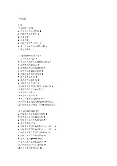
/*计算几何目录㈠点的基本运算1. 平面上两点之间距离12. 判断两点是否重合13. 矢量叉乘14. 矢量点乘25. 判断点是否在线段上26. 求一点饶某点旋转后的坐标27. 求矢量夹角2㈡线段及直线的基本运算1. 点与线段的关系32. 求点到线段所在直线垂线的垂足43. 点到线段的最近点44. 点到线段所在直线的距离45. 点到折线集的最近距离46. 判断圆是否在多边形内57. 求矢量夹角余弦58. 求线段之间的夹角59. 判断线段是否相交610.判断线段是否相交但不交在端点处611.求线段所在直线的方程612.求直线的斜率713.求直线的倾斜角714.求点关于某直线的对称点715.判断两条直线是否相交及求直线交点716.判断线段是否相交，如果相交返回交点7㈢多边形常用算法模块1. 判断多边形是否简单多边形82. 检查多边形顶点的凸凹性93. 判断多边形是否凸多边形94. 求多边形面积95. 判断多边形顶点的排列方向，方法一106. 判断多边形顶点的排列方向，方法二107. 射线法判断点是否在多边形内108. 判断点是否在凸多边形内119. 寻找点集的graham算法1210.寻找点集凸包的卷包裹法1311.判断线段是否在多边形内1412.求简单多边形的重心1513.求凸多边形的重心1714.求肯定在给定多边形内的一个点1715.求从多边形外一点出发到该多边形的切线1816.判断多边形的核是否存在19㈣圆的基本运算1 .点是否在圆内202 .求不共线的三点所确定的圆21㈤矩形的基本运算1.已知矩形三点坐标，求第4点坐标22㈥常用算法的描述22㈦补充1．两圆关系：242．判断圆是否在矩形内：243．点到平面的距离：254．点是否在直线同侧：255．镜面反射线：256．矩形包含：267．两圆交点：278．两圆公共面积：289. 圆和直线关系：2910. 内切圆：3011. 求切点：3112. 线段的左右旋：3113．公式：32*//* 需要包含的头文件*/#include <cmath >/* 常用的常量定义*/const double INF = 1E200const double EP = 1E-10const int MAXV = 300const double PI = 3.14159265/* 基本几何结构*/struct POINT{double x;double y;POINT(double a=0, double b=0) { x=a; y=b;} //constructor};struct LINESEG{POINT s;POINT e;LINESEG(POINT a, POINT b) { s=a; e=b;}LINESEG() { }};struct LINE // 直线的解析方程a*x+b*y+c=0 为统一表示，约定a >= 0{double a;double b;double c;LINE(double d1=1, double d2=-1, double d3=0) {a=d1; b=d2; c=d3;}};/*********************** ** 点的基本运算** ***********************/double dist(POINT p1,POINT p2) // 返回两点之间欧氏距离{return( sqrt( (p1.x-p2.x)*(p1.x-p2.x)+(p1.y-p2.y)*(p1.y-p2.y) ) );}bool equal_point(POINT p1,POINT p2) // 判断两个点是否重合{return ( (abs(p1.x-p2.x)<EP)&&(abs(p1.y-p2.y)<EP) );}/****************************************************************************** r=multiply(sp,ep,op),得到(sp-op)和(ep-op)的叉积r>0：ep在矢量opsp的逆时针方向；r=0：opspep三点共线；r<0：ep在矢量opsp的顺时针方向******************************************************************************* /double multiply(POINT sp,POINT ep,POINT op){return((sp.x-op.x)*(ep.y-op.y)-(ep.x-op.x)*(sp.y-op.y));}/*r=dotmultiply(p1,p2,op),得到矢量(p1-op)和(p2-op)的点积，如果两个矢量都非零矢量r<0：两矢量夹角为锐角；r=0：两矢量夹角为直角；r>0：两矢量夹角为钝角******************************************************************************* /double dotmultiply(POINT p1,POINT p2,POINT p0){return ((p1.x-p0.x)*(p2.x-p0.x)+(p1.y-p0.y)*(p2.y-p0.y));}/****************************************************************************** 判断点p是否在线段l上条件：(p在线段l所在的直线上) && (点p在以线段l为对角线的矩形内)******************************************************************************* /bool online(LINESEG l,POINT p){return( (multiply(l.e,p,l.s)==0) &&( ( (p.x-l.s.x)*(p.x-l.e.x)<=0 )&&( (p.y-l.s.y)*(p.y-l.e.y)<=0 ) ) ); }// 返回点p以点o为圆心逆时针旋转alpha(单位：弧度)后所在的位置POINT rotate(POINT o,double alpha,POINT p){POINT tp;p.x-=o.x;p.y-=o.y;tp.x=p.x*cos(alpha)-p.y*sin(alpha)+o.x;tp.y=p.y*cos(alpha)+p.x*sin(alpha)+o.y;return tp;}/* 返回顶角在o点，起始边为os，终止边为oe的夹角(单位：弧度)角度小于pi，返回正值角度大于pi，返回负值可以用于求线段之间的夹角原理：r = dotmultiply(s,e,o) / (dist(o,s)*dist(o,e))r'= multiply(s,e,o)r >= 1 angle = 0;r <= -1 angle = -PI-1<r<1 && r'>0 angle = arccos(r)-1<r<1 && r'<=0 angle = -arccos(r)*/double angle(POINT o,POINT s,POINT e){double cosfi,fi,norm;double dsx = s.x - o.x;double dsy = s.y - o.y;double dex = e.x - o.x;double dey = e.y - o.y;cosfi=dsx*dex+dsy*dey;norm=(dsx*dsx+dsy*dsy)*(dex*dex+dey*dey);cosfi /= sqrt( norm );if (cosfi >= 1.0 ) return 0;if (cosfi <= -1.0 ) return -3.1415926;fi=acos(cosfi);if (dsx*dey-dsy*dex>0) return fi; // 说明矢量os 在矢量oe的顺时针方向return -fi;}/*****************************\* ** 线段及直线的基本运算** *\*****************************//* 判断点与线段的关系,用途很广泛本函数是根据下面的公式写的，P是点C到线段AB所在直线的垂足AC dot ABr = ---------||AB||^2(Cx-Ax)(Bx-Ax) + (Cy-Ay)(By-Ay)= -------------------------------L^2r has the following meaning:r=0 P = Ar=1 P = Br<0 P is on the backward extension of ABr>1 P is on the forward extension of AB0<r<1 P is interior to AB*/double relation(POINT p,LINESEG l){LINESEG tl;tl.s=l.s;tl.e=p;return dotmultiply(tl.e,l.e,l.s)/(dist(l.s,l.e)*dist(l.s,l.e));}// 求点C到线段AB所在直线的垂足PPOINT perpendicular(POINT p,LINESEG l){double r=relation(p,l);POINT tp;tp.x=l.s.x+r*(l.e.x-l.s.x);tp.y=l.s.y+r*(l.e.y-l.s.y);return tp;}/* 求点p到线段l的最短距离,并返回线段上距该点最近的点np注意：np是线段l上到点p最近的点，不一定是垂足*/double ptolinesegdist(POINT p,LINESEG l,POINT &np){double r=relation(p,l);if(r<0){np=l.s;return dist(p,l.s);}if(r>1){np=l.e;return dist(p,l.e);}np=perpendicular(p,l);return dist(p,np);}// 求点p到线段l所在直线的距离,请注意本函数与上个函数的区别double ptoldist(POINT p,LINESEG l){return abs(multiply(p,l.e,l.s))/dist(l.s,l.e);}/* 计算点到折线集的最近距离,并返回最近点.注意：调用的是ptolineseg()函数*/double ptopointset(int vcount,POINT pointset[],POINT p,POINT &q) {int i;double cd=double(INF),td;LINESEG l;POINT tq,cq;for(i=0;i<vcount-1;i++)l.s=pointset[i];l.e=pointset[i+1];td=ptolinesegdist(p,l,tq);if(td<cd){cd=td;cq=tq;}}q=cq;return cd;}/* 判断圆是否在多边形内.ptolineseg()函数的应用2 */bool CircleInsidePolygon(int vcount,POINT center,double radius,POINT polygon[]){POINT q;double d;q.x=0;q.y=0;d=ptopointset(vcount,polygon,center,q);if(d<radius||fabs(d-radius)<EP)return true;elsereturn false;}/* 返回两个矢量l1和l2的夹角的余弦(-1 --- 1)注意：如果想从余弦求夹角的话，注意反余弦函数的定义域是从0到pi */double cosine(LINESEG l1,LINESEG l2){return (((l1.e.x-l1.s.x)*(l2.e.x-l2.s.x) +(l1.e.y-l1.s.y)*(l2.e.y-l2.s.y))/(dist(l1.e,l1.s)*dist(l2.e,l2.s))) );}// 返回线段l1与l2之间的夹角单位：弧度范围(-pi，pi)double lsangle(LINESEG l1,LINESEG l2){POINT o,s,e;o.x=o.y=0;s.x=l1.e.x-l1.s.x;s.y=l1.e.y-l1.s.y;e.x=l2.e.x-l2.s.x;e.y=l2.e.y-l2.s.y;return angle(o,s,e);// 如果线段u和v相交(包括相交在端点处)时，返回true////判断P1P2跨立Q1Q2的依据是：( P1 - Q1 ) ×( Q2 - Q1 ) * ( Q2 - Q1 ) ×( P2 - Q1 ) >= 0。

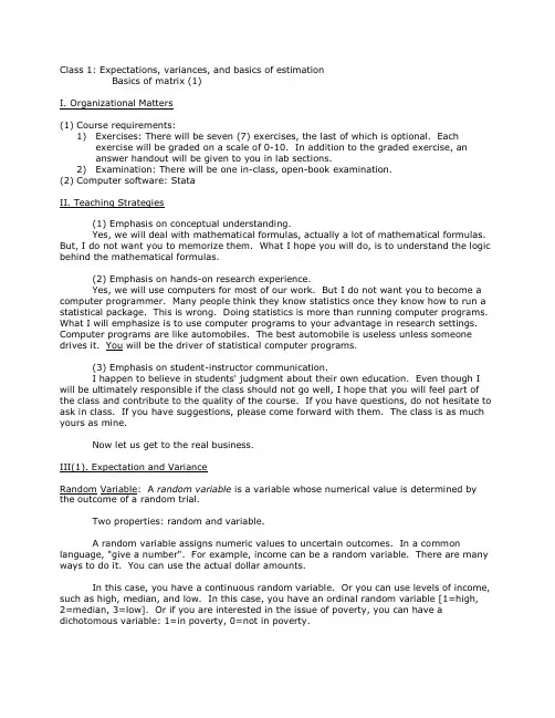
Class 1: Expectations, variances, and basics of estimationBasics of matrix (1)I. Organizational Matters(1)Course requirements:1)Exercises: There will be seven (7) exercises, the last of which is optional. Eachexercise will be graded on a scale of 0-10. In addition to the graded exercise, ananswer handout will be given to you in lab sections.2)Examination: There will be one in-class, open-book examination.(2)Computer software: StataII. Teaching Strategies(1) Emphasis on conceptual understanding.Yes, we will deal with mathematical formulas, actually a lot of mathematical formulas. But, I do not want you to memorize them. What I hope you will do, is to understand the logic behind the mathematical formulas.(2) Emphasis on hands-on research experience.Yes, we will use computers for most of our work. But I do not want you to become a computer programmer. Many people think they know statistics once they know how to run a statistical package. This is wrong. Doing statistics is more than running computer programs. What I will emphasize is to use computer programs to your advantage in research settings. Computer programs are like automobiles. The best automobile is useless unless someone drives it. You will be the driver of statistical computer programs.(3) Emphasis on student-instructor communication.I happen to believe in students' judgment about their own education. Even though I will be ultimately responsible if the class should not go well, I hope that you will feel part of the class and contribute to the quality of the course. If you have questions, do not hesitate to ask in class. If you have suggestions, please come forward with them. The class is as much yours as mine.Now let us get to the real business.III(1). Expectation and VarianceRandom Variable: A random variable is a variable whose numerical value is determined by the outcome of a random trial.Two properties: random and variable.A random variable assigns numeric values to uncertain outcomes. In a common language, "give a number". For example, income can be a random variable. There are many ways to do it. You can use the actual dollar amounts.In this case, you have a continuous random variable. Or you can use levels of income, such as high, median, and low. In this case, you have an ordinal random variable [1=high,2=median, 3=low]. Or if you are interested in the issue of poverty, you can have a dichotomous variable: 1=in poverty, 0=not in poverty.In sum, the mapping of numeric values to outcomes of events in this way is theessence of a random variable.Probability Distribution: The probability distribution for a discrete random variable Xassociates with each of the distinct outcomes x i (i = 1, 2,..., k ) a probability P (X = x i ). Cumulative Probability Distribution: The cumulative probability distribution for a discreterandom variable X provides the cumulative probabilities P (X ≤ x ) for all values x .Expected Value of Random Variable: The expected value of a discrete random variable X isdenoted by E {X } and defined:E {X } = x i i k=∑1P (x i )where : P (x i ) denotes P (X = x i ). The notation E { } (read “expectation of”) is called theexpectation operator.In common language, expectation is the mean. But the difference is that expectation is a concept for the entire population that you never observe. It is the result of the infinitenumber of repetitions. For example, if you toss a coin, the proportion of tails should be .5 in the limit. Or the expectation is .5. Most of the times you do not get the exact .5, but a number close to it.Conditional ExpectationIt is the mean of a variable conditional on the value of another random variable.Note the notation: E(Y|X).In 1996, per-capita average wages in three Chinese cities were (in RMB):Shanghai: 3,778Wuhan: 1,709Xi ’an: 1,155Variance of Random Variable: The variance of a discrete random variable X is denoted by V {X } and defined:V {X } = i k =∑1(x i - E {X })2 P (x i )where : P (x i ) denotes P (X = x i ). The notation V { } (read “variance of”) is called the variance operator.Since the variance of a random variable X is a weighted average of the squared deviations,(X - E {X })2 , it may be defined equivalently as an expected value: V {X } = E {(X - E {X })2}. An algebraically identical expression is: V {X} = E {X 2} - (E {X })2.Standard Deviation of Random Variable: The positive square root of the variance of X is called the standard deviation of X and is denoted by σ{X }:σ {X } =V X {}The notation σ{ } (read “standard deviation of”) is called the standard deviation operator. Standardized Random Variables: If X is a random variable with expected value E {X } and standard deviation σ{X }, then:Y =}{}{X X E X σ-is known as the standardized form of random variable X .Covariance: The covariance of two discrete random variables X and Y is denoted by Cov {X,Y } and defined:Cov {X, Y } = ({})({})(,)xE X y E Y P x y i j i j j i --∑∑where: P (x i , y j ) denotes P Xx Y y i j (=⋂= ) The notation of Cov { , } (read “covariance of”) is called the covariance operator .When X and Y are independent, Cov {X, Y } = 0.Cov {X, Y } = E {(X - E {X })(Y - E {Y })}; Cov {X, Y } = E {XY } - E {X }E {Y }(Variance is a special case of covariance.)Coefficient of Correlation: The coefficient of correlation of two random variables X and Y isdenoted by ρ{X,Y } (Greek rho) and defined:ρσσ{,}{,}{}{}X Y Cov X Y X Y =where: σ{X } is the standard deviation of X; σ{Y } is the standard deviation of Y; Cov is the covariance of X and Y.Sum and Difference of Two Random Variables: If X and Y are two random variables, then the expected value and the variance of X + Y are as follows:Expected Value : E {X+Y } = E {X } + E {Y };Variance : V {X+Y } = V {X } + V {Y }+ 2 Cov (X,Y ).If X and Y are two random variables, then the expected value and the variance of X - Y are as follows:Expected Value : E {X - Y } = E {X } - E {Y };Variance : V {X - Y } = V {X } + V {Y } - 2 Cov (X,Y ).Sum of More Than Two Independent Random Variables: If T = X 1 + X 2 + ... + X s is the sumof s independent random variables, then the expected value and the variance of T are as follows:Expected Value: E T E X i i s {}{}==∑1; Variance: V T V X i i s {}{}==∑1III(2). Properties of Expectations and Covariances:(1) Properties of Expectations under Simple Algebraic Operations)()(x bE a bX a E +=+This says that a linear transformation is retained after taking an expectation.bX a X +=*is called rescaling: a is the location parameter, b is the scale parameter.Special cases are:For a constant: a a E =)(For a different scale: )()(X E b bX E =, e.g., transforming the scale of dollars into thescale of cents.(2) Properties of Variances under Simple Algebraic Operations)()(2X V b bX a V =+This says two things: (1) Adding a constant to a variable does not change the variance of the variable; reason: the definition of variance controls for the mean of the variable[graphics]. (2) Multiplying a constant to a variable changes the variance of the variable by a factor of the constant squared; this is to easy prove, and I will leave it to you. This is the reason why we often use standard deviation instead of variance2x x σσ=is of the same scale as x.(3) Properties of Covariance under Simple Algebraic OperationsCov(a + bX, c + dY) = bd Cov(X,Y).Again, only scale matters, location does not.(4) Properties of Correlation under Simple Algebraic OperationsI will leave this as part of your first exercise: ),(),(Y X dY c bX a ρρ=++That is, neither scale nor location affects correlation.IV: Basics of matrix.1. DefinitionsA. MatricesToday, I would like to introduce the basics of matrix algebra. A matrix is a rectangular array of elements arranged in rows and columns:11121211.......m n nm x x x x X x x ⎡⎤⎢⎥⎢⎥=⎢⎥⎢⎥⎣⎦Index: row index, column index.Dimension: number of rows x number of columns (n x m)Elements: are denoted in small letters with subscripts.An example is the spreadsheet that records the grades for your home work in the following way:Name 1st 2nd ....6thA 7 10 (9)B 6 5 (8)... ... ......Z 8 9 (8)This is a matrix.Notation: I will use Capital Letters for Matrices.B. VectorsVectors are special cases of matrices:If the dimension of a matrix is n x 1, it is a column vector:⎥⎥⎥⎥⎦⎤⎢⎢⎢⎢⎣⎡=n x x x x (21)If the dimension is 1 x m, it is a row vector: y' = | 1y 2y .... m y |Notation: small underlined letters for column vectors (in lecture notes)C. TransposeThe transpose of a matrix is another matrix with positions of rows and columns beingexchanged symmetrically.For example: if⎥⎥⎥⎥⎦⎤⎢⎢⎢⎢⎣⎡=⨯nm n m m n x x x x x x X 12111211)( (1121112)()1....'...n m n m nm x x x x X x x ⨯⎡⎤⎢⎥⎢⎥=⎢⎥⎢⎥⎣⎦It is easy to see that a row vector and a column vector are transposes of each other. 2. Matrix Addition and SubtractionAdditions and subtraction of two matrices are possible only when the matrices have the same dimension. In this case, addition or subtraction of matrices forms another matrix whoseelements consist of the sum, or difference, of the corresponding elements of the two matrices.⎥⎥⎥⎥⎦⎤⎢⎢⎢⎢⎣⎡±±±±±=Y ±X mn nm n n m m y x y x y x y x y x (11)2121111111 Examples:⎥⎦⎤⎢⎣⎡=A ⨯4321)22(⎥⎦⎤⎢⎣⎡=B ⨯1111)22(⎥⎦⎤⎢⎣⎡=B +A =⨯5432)22(C 3. Matrix MultiplicationA. Multiplication of a scalar and a matrixMultiplying a scalar to a matrix is equivalent to multiplying the scalar to each of the elements of the matrix.11121211Χ...m n nm cx c cx cx ⎢⎥⎢⎥=⎢⎥⎢⎥⎣⎦ B. Multiplication of a Matrix by a Matrix (Inner Product)The inner product of matrix X (a x b) and matrix Y (c x d) exists if b is equal to c. The inner product is a new matrix with the dimension (a x d). The element of the new matrix Z is:c∑=kj ik ijy x zk=1Note that XY and YX are very different. Very often, only one of the inner products (XY and YX) exists.Example:⎥⎦⎤⎢⎣⎡=4321)22(x A⎥⎦⎤⎢⎣⎡=10)12(x BBA does not exist. AB has the dimension 2x1⎥⎦⎤⎢⎣⎡=42ABOther examples:If )53(x A , )35(x B , what is the dimension of AB? (3x3)If )53(x A , )35(x B , what is the dimension of BA? (5x5)If )51(x A , )15(x B , what is the dimension of AB? (1x1, scalar)If )53(x A , )15(x B , what is the dimension of BA? (nonexistent)4. Special MatricesA. Square Matrix)(n n A ⨯B. Symmetric MatrixA special case of square matrix.For )(n n A ⨯, ji ij a a =. All i, j .A' = AC. Diagonal MatrixA special case of symmetric matrix⎥⎥⎥⎥⎦⎢⎢⎢⎢⎣=X nn x x 0 (2211)D. Scalar Matrix0....0c c c c ⎡⎤⎢⎥⎢⎥=I ⎢⎥⎢⎥⎣⎦E. Identity MatrixA special case of scalar matrix⎥⎥⎥⎥⎦⎤⎢⎢⎢⎢⎣⎡=I 10 (101)Important: for r r A ⨯AI = IA = AF. Null (Zero) MatrixAnother special case of scalar matrix⎥⎥⎥⎥⎦⎤⎢⎢⎢⎢⎣⎡=O 00 (000)From A to E or F, cases are nested from being more general towards being more specific.G. Idempotent MatrixLet A be a square symmetric matrix. A is idempotent if ....32=A =A =AH. Vectors and Matrices with elements being oneA column vector with all elements being 1,⎥⎥⎥⎥⎦⎤⎢⎢⎢⎢⎣⎡=⨯1 (111)r A matrix with all elements being 1, ⎥⎥⎥⎥⎦⎤⎢⎢⎢⎢⎣⎡=⨯1...1...111...11rr J Examples let 1 be a vector of n 1's: )1(1⨯n 1'1 = )11(⨯n11' = )(n n J ⨯I. Zero Vector A zero vector is ⎥⎥⎥⎥⎦⎤⎢⎢⎢⎢⎣⎡=⨯0 (001)r 5. Rank of a MatrixThe maximum number of linearly independent rows is equal to the maximum number oflinearly independent columns. This unique number is defined to be the rank of the matrix. For example,⎥⎥⎥⎦⎤⎢⎢⎢⎣⎡=B 542211014321 Because row 3 = row 1 + row 2, the 3rd row is linearly dependent on rows 1 and 2. The maximum number of independent rows is 2. Let us have a new matrix:⎥⎦⎤⎢⎣⎡=B 11014321* Singularity: if a square matrix A of dimension ()n n ⨯has rank n, the matrix is nonsingular. If the rank is less than n, the matrix is then singular.。

acm-icpc暑期课_最短路北京⼤学暑期课《ACM/ICPC 竞赛训练》最短路算法本讲义为四处抄袭后改编⽽成，来源已不可考。

仅⽤于内部授课北京⼤学信息学院郭炜 guo_wei@/doc/d83c4f84bb68a98270fefa4a.html/doc/d83c4f84bb68a98270fefa4a.html /guoweiofpkuDijkstra 算法●解决⽆负权边的带权有向图或⽆向图的单源最短路问题●贪⼼思想，若离源点s 前k-1近的点已经被确定，构成点集P ，那么从s 到离s 第k 近的点t 的最短路径，{s,p 1,p 2…p i ,t}满⾜s,p 1,p 2…p i ∈P 。

●否则假设pi ?P ，则因为边权⾮负，pi 到t 的路径≥0，则d[pi]≤d[t],pi 才是第k 近。

将pi 看作t ，重复上⾯过程，最终⼀定会有找不到pi 的情况●d[i]=min(d[p i ]+cost(p i ,i)),i ?P,p i ∈P d[t]=min(d[i]) ,i ?P基本思想●初始令d[s]=0，d[i]=+∞，P=?●找到点i?P，且d[i]最⼩●把i添⼊P，对于任意j?P，若d[i]+cost(i,j)d[j]=d[i]+cost(i,j)。

●⽤邻接表，不优化，时间复杂度O(V2+E)●Dijkstra+堆的时间复杂度 o(ElgV)●⽤斐波那契堆可以做到O(VlogV+E)●若要输出路径，则设置prev数组记录每个节点的前趋点，在d[i]更新时更新prev[i]4 23 150200200 100080005000v Dist[v]0 01234 50100001000300025025082505250源点0加⼊P后：Dijkstra's AlgorithmDijkstra 算法也适⽤于⽆向图。

但不适⽤于有负权边的图。

231-234d[1,2] = 2但⽤Dijkstra 算法求得 d[1,2] = 3有N个孩⼦（N<=3000)分糖果。

北京大学暑期课《ACM/ICPC竞赛训练》北京大学信息学院郭炜guo_wei@/guoweiofpku课程网页：/summerschool/pku_acm_train.htm信息科学技术学院《程序设计与算法》ACM/ICPC中的数学郭炜/林舒( a + b ) mod c =((a mod c) + (b mod c)) mod c( a * b ) mod c =((a mod c) * (b mod c)) mod c消去律：若 gcd(c,p) = 1,则ac ≡ bc mod p => a ≡ b mod p消去律证明：ac ≡ bc mod p => ac = bc + kp => c(a-b) = kpc和p没有除1以外的公因子 =>1) c能整除k 或 2) a = b如果2不成立，则c|kpc和p没有公因子 => c|k，所以k = ck'=> c(a-b)=kp可以表示为c(a-b) =ck'p因此a-b = k'p，得出a ≡ b mod pint Pow(int a,int b){ //快速求a^b ，复杂度 log(b)if(b == 0)return 1;if(b & 1) { //b是奇数return a * Pow(a,b-1);}else {int t = Pow(a,b/2);return t * t;}}int Pow(int a,int b){ //快速求a^b ，复杂度 log(b) int result = 1;int base = a;while(b) {if( b & 1)result *= base;base *= base;b >>= 1;}return result;}快速幂取模int PowMod(int a,int b,int c){//快速求 a^b % c ，要避免计算中间结果溢出int result = 1;int base = a%c;while(b) {if( b & 1)result = (result * base)%c;base = (base * base) % c;b >>= 1;}return result;}Sn= a+a2+...+a n要求 Snmod p如果用公式算，可能溢出，因此用二分法求1) 若 n是偶数Sn= a+...+a n/2 + a n/2+1 + a n/2+2 +...+ a n/2+n/2 =(a+...+a n/2) + a n/2(a+...+a n/2)=Sn/2+ a n/2Sn/2=(1+a n/2)Sn/22) 若n是奇数= a+...+a(n-1)/2 + a(n-1)/2+1 +...Sn+ a(n-1)/2+(n-1)/2 + a(n-1)/2+(n-1)/2 + 1 =S+ a(n-1)/2(a+...+a(n-1)/2)+a n (n-1)/2+a n=(1+a(n-1)/2)S(n-1)/2等比数列二分求和取模int PowSumMod(int a,int n,int p){// return (a+ a^2 + ... + a^n) Mod p;if( n == 1)return a%p;if( n %2 == 0)return (1+PowMod(a,n/2,p))*PowSumMod(a,n/2,p) % p;elsereturn ((1+PowMod(a,(n-1)/2,p)) * PowSumMod(a,(n-1)/2,p) + PowMod(a,n,p)) % p;}POJ3233 Matrix Power Series矩阵快速幂+等比数列二分求和取模给一个n×n的整数矩阵A和正整数k,m, 令S = A + A2 + A3+ … +A k求 S mod m (S的每个都 mod m)n (n≤ 30),k (k≤ 109) and m (m < 104).struct Matrix{T a[32][32];int r; //行列数Mat(int rr):r(rr) { }void MakeI() { //变为单位矩阵memset(a,0,sizeof(a));for(int i = 0;i < r; ++i)a[i][i] = 1;}};Matrix Pow(const Matrix & m,int k,int p){ //求m k mod pint r = m.r;Matrix result(r);result.MakeI(); //MakeI是将result变为单位矩阵Matrix base = m;while(k) {if( k & 1)result = Product(result,base,p); //result*base mod pk >>= 1;base = Product(base,base,p);}return result;} 14欧几里得算法求最大公约数int Gcd(int a,int b){if( b == 0)return a;return Gcd(b,a%b);}最小公倍数：lcm(a,b) = a*b/gcd(a,b)ax+by=gcd(a,b) 有整数解(x,y)<=>bx+(a%b)y = gcd(a,b) 有整数解(x1,y1)，且x = y1, y = x1-[a/b]*y1因此，可以在求gcd(a,b)的同时，对 ax+by=gcd(a,b)求解int GcdEx(int a,int b,int &x ,int & y) //求 ax+by=gcd(a,b)的整数解,返回gcd(a,b) {if( b == 0) {x = 1;y = 0;return a;}int x1,y1;int gcd = GcdEx(b,a%b,x1,y1);x = y1;y = x1 - a/b * y1;return gcd;}• ax+by=c 有解的充要条件是 gcd(a,b)|c•设 d = gcd(a,b), k = c/d，ax+by = d的解是 (x1,y1) 则ax+by = c的解集是：x = k*x1 + t*(b/d)y = k*y1 – t*(a/d) t为任意整数18•求ax≡c(mod b)等价于求 ax+by = c •设 d = gcd(a,b), k = c/d，ax+by = d的解是 (x1,y1) 则•ax≡c(mod b) 的解集是：x = k*x1 + t*(b/d) t为任意整数其中模b不同的解共有 d 个，为：x = k*x1 + t*(b/d) t=0,1,..d-1•求ax≡c(mod b) 的最小非负整数解：令 ans = k * x1;s = b/d;则 x = ans + t*s t为任意整数则最小非负整数解是：(ans%s + s)%s•对下面的循环：for (variable = A; variable != B; variable += C)statement;A,B,C和variable都是K(K<=32)比特的无符号数,+=运算的结果也是K比特的无符号数，给定 A,B,C和K，问循环执行多少次。