计量经济学课件英文版 伍德里奇

T his appendix derives various results for ordinary least squares estimation of themultiple linear regression model using matrix notation and matrix algebra (see Appendix D for a summary). The material presented here is much more ad-vanced than that in the text.E.1THE MODEL AND ORDINARY LEAST SQUARES ESTIMATIONThroughout this appendix,we use the t subscript to index observations and an n to denote the sample size. It is useful to write the multiple linear regression model with k parameters as follows:y t ϭ␤1ϩ␤2x t 2ϩ␤3x t 3ϩ… ϩ␤k x tk ϩu t ,t ϭ 1,2,…,n ,(E.1)where y t is the dependent variable for observation t ,and x tj ,j ϭ 2,3,…,k ,are the inde-pendent variables. Notice how our labeling convention here differs from the text:we call the intercept ␤1and let ␤2,…,␤k denote the slope parameters. This relabeling is not important,but it simplifies the matrix approach to multiple regression.For each t ,define a 1 ϫk vector,x t ϭ(1,x t 2,…,x tk ),and let ␤ϭ(␤1,␤2,…,␤k )Јbe the k ϫ1 vector of all parameters. Then,we can write (E.1) asy t ϭx t ␤ϩu t ,t ϭ 1,2,…,n .(E.2)[Some authors prefer to define x t as a column vector,in which case,x t is replaced with x t Јin (E.2). Mathematically,it makes more sense to define it as a row vector.] We can write (E.2) in full matrix notation by appropriately defining data vectors and matrices. Let y denote the n ϫ1 vector of observations on y :the t th element of y is y t .Let X be the n ϫk vector of observations on the explanatory variables. In other words,the t th row of X consists of the vector x t . Equivalently,the (t ,j )th element of X is simply x tj :755A p p e n d i x EThe Linear Regression Model inMatrix Formn X ϫ k ϵϭ .Finally,let u be the n ϫ 1 vector of unobservable disturbances. Then,we can write (E.2)for all n observations in matrix notation :y ϭX ␤ϩu .(E.3)Remember,because X is n ϫ k and ␤is k ϫ 1,X ␤is n ϫ 1.Estimation of ␤proceeds by minimizing the sum of squared residuals,as in Section3.2. Define the sum of squared residuals function for any possible k ϫ 1 parameter vec-tor b asSSR(b ) ϵ͚nt ϭ1(y t Ϫx t b )2.The k ϫ 1 vector of ordinary least squares estimates,␤ˆϭ(␤ˆ1,␤ˆ2,…,␤ˆk )؅,minimizes SSR(b ) over all possible k ϫ 1 vectors b . This is a problem in multivariable calculus.For ␤ˆto minimize the sum of squared residuals,it must solve the first order conditionѨSSR(␤ˆ)/Ѩb ϵ0.(E.4)Using the fact that the derivative of (y t Ϫx t b )2with respect to b is the 1ϫ k vector Ϫ2(y t Ϫx t b )x t ,(E.4) is equivalent to͚nt ϭ1xt Ј(y t Ϫx t ␤ˆ) ϵ0.(E.5)(We have divided by Ϫ2 and taken the transpose.) We can write this first order condi-tion as͚nt ϭ1(y t Ϫ␤ˆ1Ϫ␤ˆ2x t 2Ϫ… Ϫ␤ˆk x tk ) ϭ0͚nt ϭ1x t 2(y t Ϫ␤ˆ1Ϫ␤ˆ2x t 2Ϫ… Ϫ␤ˆk x tk ) ϭ0...͚nt ϭ1x tk (y t Ϫ␤ˆ1Ϫ␤ˆ2x t 2Ϫ… Ϫ␤ˆk x tk ) ϭ0,which,apart from the different labeling convention,is identical to the first order condi-tions in equation (3.13). We want to write these in matrix form to make them more use-ful. Using the formula for partitioned multiplication in Appendix D,we see that (E.5)is equivalent to΅1x 12x 13...x 1k1x 22x 23...x 2k...1x n 2x n 3...x nk ΄΅x 1x 2...x n ΄Appendix E The Linear Regression Model in Matrix Form756Appendix E The Linear Regression Model in Matrix FormXЈ(yϪX␤ˆ) ϭ0(E.6) or(XЈX)␤ˆϭXЈy.(E.7)It can be shown that (E.7) always has at least one solution. Multiple solutions do not help us,as we are looking for a unique set of OLS estimates given our data set. Assuming that the kϫ k symmetric matrix XЈX is nonsingular,we can premultiply both sides of (E.7) by (XЈX)Ϫ1to solve for the OLS estimator ␤ˆ:␤ˆϭ(XЈX)Ϫ1XЈy.(E.8)This is the critical formula for matrix analysis of the multiple linear regression model. The assumption that XЈX is invertible is equivalent to the assumption that rank(X) ϭk, which means that the columns of X must be linearly independent. This is the matrix ver-sion of MLR.4 in Chapter 3.Before we continue,(E.8) warrants a word of warning. It is tempting to simplify the formula for ␤ˆas follows:␤ˆϭ(XЈX)Ϫ1XЈyϭXϪ1(XЈ)Ϫ1XЈyϭXϪ1y.The flaw in this reasoning is that X is usually not a square matrix,and so it cannot be inverted. In other words,we cannot write (XЈX)Ϫ1ϭXϪ1(XЈ)Ϫ1unless nϭk,a case that virtually never arises in practice.The nϫ 1 vectors of OLS fitted values and residuals are given byyˆϭX␤ˆ,uˆϭyϪyˆϭyϪX␤ˆ.From (E.6) and the definition of uˆ,we can see that the first order condition for ␤ˆis the same asXЈuˆϭ0.(E.9) Because the first column of X consists entirely of ones,(E.9) implies that the OLS residuals always sum to zero when an intercept is included in the equation and that the sample covariance between each independent variable and the OLS residuals is zero. (We discussed both of these properties in Chapter 3.)The sum of squared residuals can be written asSSR ϭ͚n tϭ1uˆt2ϭuˆЈuˆϭ(yϪX␤ˆ)Ј(yϪX␤ˆ).(E.10)All of the algebraic properties from Chapter 3 can be derived using matrix algebra. For example,we can show that the total sum of squares is equal to the explained sum of squares plus the sum of squared residuals [see (3.27)]. The use of matrices does not pro-vide a simpler proof than summation notation,so we do not provide another derivation.757The matrix approach to multiple regression can be used as the basis for a geometri-cal interpretation of regression. This involves mathematical concepts that are even more advanced than those we covered in Appendix D. [See Goldberger (1991) or Greene (1997).]E.2FINITE SAMPLE PROPERTIES OF OLSDeriving the expected value and variance of the OLS estimator ␤ˆis facilitated by matrix algebra,but we must show some care in stating the assumptions.A S S U M P T I O N E.1(L I N E A R I N P A R A M E T E R S)The model can be written as in (E.3), where y is an observed nϫ 1 vector, X is an nϫ k observed matrix, and u is an nϫ 1 vector of unobserved errors or disturbances.A S S U M P T I O N E.2(Z E R O C O N D I T I O N A L M E A N)Conditional on the entire matrix X, each error ut has zero mean: E(ut͉X) ϭ0, tϭ1,2,…,n.In vector form,E(u͉X) ϭ0.(E.11) This assumption is implied by MLR.3 under the random sampling assumption,MLR.2.In time series applications,Assumption E.2 imposes strict exogeneity on the explana-tory variables,something discussed at length in Chapter 10. This rules out explanatory variables whose future values are correlated with ut; in particular,it eliminates laggeddependent variables. Under Assumption E.2,we can condition on the xtjwhen we com-pute the expected value of ␤ˆ.A S S U M P T I O N E.3(N O P E R F E C T C O L L I N E A R I T Y) The matrix X has rank k.This is a careful statement of the assumption that rules out linear dependencies among the explanatory variables. Under Assumption E.3,XЈX is nonsingular,and so ␤ˆis unique and can be written as in (E.8).T H E O R E M E.1(U N B I A S E D N E S S O F O L S)Under Assumptions E.1, E.2, and E.3, the OLS estimator ␤ˆis unbiased for ␤.P R O O F:Use Assumptions E.1 and E.3 and simple algebra to write␤ˆϭ(XЈX)Ϫ1XЈyϭ(XЈX)Ϫ1XЈ(X␤ϩu)ϭ(XЈX)Ϫ1(XЈX)␤ϩ(XЈX)Ϫ1XЈuϭ␤ϩ(XЈX)Ϫ1XЈu,(E.12)where we use the fact that (XЈX)Ϫ1(XЈX) ϭIk . Taking the expectation conditional on X givesAppendix E The Linear Regression Model in Matrix Form 758E(␤ˆ͉X)ϭ␤ϩ(XЈX)Ϫ1XЈE(u͉X)ϭ␤ϩ(XЈX)Ϫ1XЈ0ϭ␤,because E(u͉X) ϭ0under Assumption E.2. This argument clearly does not depend on the value of ␤, so we have shown that ␤ˆis unbiased.To obtain the simplest form of the variance-covariance matrix of ␤ˆ,we impose the assumptions of homoskedasticity and no serial correlation.A S S U M P T I O N E.4(H O M O S K E D A S T I C I T Y A N DN O S E R I A L C O R R E L A T I O N)(i) Var(ut͉X) ϭ␴2, t ϭ 1,2,…,n. (ii) Cov(u t,u s͉X) ϭ0, for all t s. In matrix form, we canwrite these two assumptions asVar(u͉X) ϭ␴2I n,(E.13)where Inis the nϫ n identity matrix.Part (i) of Assumption E.4 is the homoskedasticity assumption:the variance of utcan-not depend on any element of X,and the variance must be constant across observations, t. Part (ii) is the no serial correlation assumption:the errors cannot be correlated across observations. Under random sampling,and in any other cross-sectional sampling schemes with independent observations,part (ii) of Assumption E.4 automatically holds. For time series applications,part (ii) rules out correlation in the errors over time (both conditional on X and unconditionally).Because of (E.13),we often say that u has scalar variance-covariance matrix when Assumption E.4 holds. We can now derive the variance-covariance matrix of the OLS estimator.T H E O R E M E.2(V A R I A N C E-C O V A R I A N C EM A T R I X O F T H E O L S E S T I M A T O R)Under Assumptions E.1 through E.4,Var(␤ˆ͉X) ϭ␴2(XЈX)Ϫ1.(E.14)P R O O F:From the last formula in equation (E.12), we haveVar(␤ˆ͉X) ϭVar[(XЈX)Ϫ1XЈu͉X] ϭ(XЈX)Ϫ1XЈ[Var(u͉X)]X(XЈX)Ϫ1.Now, we use Assumption E.4 to getVar(␤ˆ͉X)ϭ(XЈX)Ϫ1XЈ(␴2I n)X(XЈX)Ϫ1ϭ␴2(XЈX)Ϫ1XЈX(XЈX)Ϫ1ϭ␴2(XЈX)Ϫ1.Appendix E The Linear Regression Model in Matrix Form759Formula (E.14) means that the variance of ␤ˆj (conditional on X ) is obtained by multi-plying ␴2by the j th diagonal element of (X ЈX )Ϫ1. For the slope coefficients,we gave an interpretable formula in equation (3.51). Equation (E.14) also tells us how to obtain the covariance between any two OLS estimates:multiply ␴2by the appropriate off diago-nal element of (X ЈX )Ϫ1. In Chapter 4,we showed how to avoid explicitly finding covariances for obtaining confidence intervals and hypotheses tests by appropriately rewriting the model.The Gauss-Markov Theorem,in its full generality,can be proven.T H E O R E M E .3 (G A U S S -M A R K O V T H E O R E M )Under Assumptions E.1 through E.4, ␤ˆis the best linear unbiased estimator.P R O O F :Any other linear estimator of ␤can be written as␤˜ ϭA Јy ,(E.15)where A is an n ϫ k matrix. In order for ␤˜to be unbiased conditional on X , A can consist of nonrandom numbers and functions of X . (For example, A cannot be a function of y .) To see what further restrictions on A are needed, write␤˜ϭA Ј(X ␤ϩu ) ϭ(A ЈX )␤ϩA Јu .(E.16)Then,E(␤˜͉X )ϭA ЈX ␤ϩE(A Јu ͉X )ϭA ЈX ␤ϩA ЈE(u ͉X ) since A is a function of XϭA ЈX ␤since E(u ͉X ) ϭ0.For ␤˜to be an unbiased estimator of ␤, it must be true that E(␤˜͉X ) ϭ␤for all k ϫ 1 vec-tors ␤, that is,A ЈX ␤ϭ␤for all k ϫ 1 vectors ␤.(E.17)Because A ЈX is a k ϫ k matrix, (E.17) holds if and only if A ЈX ϭI k . Equations (E.15) and (E.17) characterize the class of linear, unbiased estimators for ␤.Next, from (E.16), we haveVar(␤˜͉X ) ϭA Ј[Var(u ͉X )]A ϭ␴2A ЈA ,by Assumption E.4. Therefore,Var(␤˜͉X ) ϪVar(␤ˆ͉X )ϭ␴2[A ЈA Ϫ(X ЈX )Ϫ1]ϭ␴2[A ЈA ϪA ЈX (X ЈX )Ϫ1X ЈA ] because A ЈX ϭI kϭ␴2A Ј[I n ϪX (X ЈX )Ϫ1X Ј]Aϵ␴2A ЈMA ,where M ϵI n ϪX (X ЈX )Ϫ1X Ј. Because M is symmetric and idempotent, A ЈMA is positive semi-definite for any n ϫ k matrix A . This establishes that the OLS estimator ␤ˆis BLUE. How Appendix E The Linear Regression Model in Matrix Form 760Appendix E The Linear Regression Model in Matrix Formis this significant? Let c be any kϫ 1 vector and consider the linear combination cЈ␤ϭc1␤1ϩc2␤2ϩ… ϩc k␤k, which is a scalar. The unbiased estimators of cЈ␤are cЈ␤ˆand cЈ␤˜. ButVar(c␤˜͉X) ϪVar(cЈ␤ˆ͉X) ϭcЈ[Var(␤˜͉X) ϪVar(␤ˆ͉X)]cՆ0,because [Var(␤˜͉X) ϪVar(␤ˆ͉X)] is p.s.d. Therefore, when it is used for estimating any linear combination of ␤, OLS yields the smallest variance. In particular, Var(␤ˆj͉X) ՅVar(␤˜j͉X) for any other linear, unbiased estimator of ␤j.The unbiased estimator of the error variance ␴2can be written as␴ˆ2ϭuˆЈuˆ/(n Ϫk),where we have labeled the explanatory variables so that there are k total parameters, including the intercept.T H E O R E M E.4(U N B I A S E D N E S S O F␴ˆ2)Under Assumptions E.1 through E.4, ␴ˆ2is unbiased for ␴2: E(␴ˆ2͉X) ϭ␴2for all ␴2Ͼ0. P R O O F:Write uˆϭyϪX␤ˆϭyϪX(XЈX)Ϫ1XЈyϭM yϭM u, where MϭI nϪX(XЈX)Ϫ1XЈ,and the last equality follows because MXϭ0. Because M is symmetric and idempotent,uˆЈuˆϭuЈMЈM uϭuЈM u.Because uЈM u is a scalar, it equals its trace. Therefore,ϭE(uЈM u͉X)ϭE[tr(uЈM u)͉X] ϭE[tr(M uuЈ)͉X]ϭtr[E(M uuЈ|X)] ϭtr[M E(uuЈ|X)]ϭtr(M␴2I n) ϭ␴2tr(M) ϭ␴2(nϪ k).The last equality follows from tr(M) ϭtr(I) Ϫtr[X(XЈX)Ϫ1XЈ] ϭnϪtr[(XЈX)Ϫ1XЈX] ϭnϪn) ϭnϪk. Therefore,tr(IkE(␴ˆ2͉X) ϭE(uЈM u͉X)/(nϪ k) ϭ␴2.E.3STATISTICAL INFERENCEWhen we add the final classical linear model assumption,␤ˆhas a multivariate normal distribution,which leads to the t and F distributions for the standard test statistics cov-ered in Chapter 4.A S S U M P T I O N E.5(N O R M A L I T Y O F E R R O R S)are independent and identically distributed as Normal(0,␴2). Conditional on X, the utEquivalently, u given X is distributed as multivariate normal with mean zero and variance-covariance matrix ␴2I n: u~ Normal(0,␴2I n).761Appendix E The Linear Regression Model in Matrix Form Under Assumption E.5,each uis independent of the explanatory variables for all t. Inta time series setting,this is essentially the strict exogeneity assumption.T H E O R E M E.5(N O R M A L I T Y O F␤ˆ)Under the classical linear model Assumptions E.1 through E.5, ␤ˆconditional on X is dis-tributed as multivariate normal with mean ␤and variance-covariance matrix ␴2(XЈX)Ϫ1.Theorem E.5 is the basis for statistical inference involving ␤. In fact,along with the properties of the chi-square,t,and F distributions that we summarized in Appendix D, we can use Theorem E.5 to establish that t statistics have a t distribution under Assumptions E.1 through E.5 (under the null hypothesis) and likewise for F statistics. We illustrate with a proof for the t statistics.T H E O R E M E.6Under Assumptions E.1 through E.5,(␤ˆjϪ␤j)/se(␤ˆj) ~ t nϪk,j ϭ 1,2,…,k.P R O O F:The proof requires several steps; the following statements are initially conditional on X. First, by Theorem E.5, (␤ˆjϪ␤j)/sd(␤ˆ) ~ Normal(0,1), where sd(␤ˆj) ϭ␴͙ෆc jj, and c jj is the j th diagonal element of (XЈX)Ϫ1. Next, under Assumptions E.1 through E.5, conditional on X,(n Ϫ k)␴ˆ2/␴2~ ␹2nϪk.(E.18)This follows because (nϪk)␴ˆ2/␴2ϭ(u/␴)ЈM(u/␴), where M is the nϫn symmetric, idem-potent matrix defined in Theorem E.4. But u/␴~ Normal(0,I n) by Assumption E.5. It follows from Property 1 for the chi-square distribution in Appendix D that (u/␴)ЈM(u/␴) ~ ␹2nϪk (because M has rank nϪk).We also need to show that ␤ˆand ␴ˆ2are independent. But ␤ˆϭ␤ϩ(XЈX)Ϫ1XЈu, and ␴ˆ2ϭuЈM u/(nϪk). Now, [(XЈX)Ϫ1XЈ]Mϭ0because XЈMϭ0. It follows, from Property 5 of the multivariate normal distribution in Appendix D, that ␤ˆand M u are independent. Since ␴ˆ2is a function of M u, ␤ˆand ␴ˆ2are also independent.Finally, we can write(␤ˆjϪ␤j)/se(␤ˆj) ϭ[(␤ˆjϪ␤j)/sd(␤ˆj)]/(␴ˆ2/␴2)1/2,which is the ratio of a standard normal random variable and the square root of a ␹2nϪk/(nϪk) random variable. We just showed that these are independent, and so, by def-inition of a t random variable, (␤ˆjϪ␤j)/se(␤ˆj) has the t nϪk distribution. Because this distri-bution does not depend on X, it is the unconditional distribution of (␤ˆjϪ␤j)/se(␤ˆj) as well.From this theorem,we can plug in any hypothesized value for ␤j and use the t statistic for testing hypotheses,as usual.Under Assumptions E.1 through E.5,we can compute what is known as the Cramer-Rao lower bound for the variance-covariance matrix of unbiased estimators of ␤(again762conditional on X ) [see Greene (1997,Chapter 4)]. This can be shown to be ␴2(X ЈX )Ϫ1,which is exactly the variance-covariance matrix of the OLS estimator. This implies that ␤ˆis the minimum variance unbiased estimator of ␤(conditional on X ):Var(␤˜͉X ) ϪVar(␤ˆ͉X ) is positive semi-definite for any other unbiased estimator ␤˜; we no longer have to restrict our attention to estimators linear in y .It is easy to show that the OLS estimator is in fact the maximum likelihood estima-tor of ␤under Assumption E.5. For each t ,the distribution of y t given X is Normal(x t ␤,␴2). Because the y t are independent conditional on X ,the likelihood func-tion for the sample is obtained from the product of the densities:͟nt ϭ1(2␲␴2)Ϫ1/2exp[Ϫ(y t Ϫx t ␤)2/(2␴2)].Maximizing this function with respect to ␤and ␴2is the same as maximizing its nat-ural logarithm:͚nt ϭ1[Ϫ(1/2)log(2␲␴2) Ϫ(yt Ϫx t ␤)2/(2␴2)].For obtaining ␤ˆ,this is the same as minimizing͚nt ϭ1(y t Ϫx t ␤)2—the division by 2␴2does not affect the optimization—which is just the problem that OLS solves. The esti-mator of ␴2that we have used,SSR/(n Ϫk ),turns out not to be the MLE of ␴2; the MLE is SSR/n ,which is a biased estimator. Because the unbiased estimator of ␴2results in t and F statistics with exact t and F distributions under the null,it is always used instead of the MLE.SUMMARYThis appendix has provided a brief discussion of the linear regression model using matrix notation. This material is included for more advanced classes that use matrix algebra,but it is not needed to read the text. In effect,this appendix proves some of the results that we either stated without proof,proved only in special cases,or proved through a more cumbersome method of proof. Other topics—such as asymptotic prop-erties,instrumental variables estimation,and panel data models—can be given concise treatments using matrices. Advanced texts in econometrics,including Davidson and MacKinnon (1993),Greene (1997),and Wooldridge (1999),can be consulted for details.KEY TERMSAppendix E The Linear Regression Model in Matrix Form 763First Order Condition Matrix Notation Minimum Variance Unbiased Scalar Variance-Covariance MatrixVariance-Covariance Matrix of the OLS EstimatorPROBLEMSE.1Let x t be the 1ϫ k vector of explanatory variables for observation t . Show that the OLS estimator ␤ˆcan be written as␤ˆϭΘ͚n tϭ1xt Јx t ΙϪ1Θ͚nt ϭ1xt Јy t Ι.Dividing each summation by n shows that ␤ˆis a function of sample averages.E.2Let ␤ˆbe the k ϫ 1 vector of OLS estimates.(i)Show that for any k ϫ 1 vector b ,we can write the sum of squaredresiduals asSSR(b ) ϭu ˆЈu ˆϩ(␤ˆϪb )ЈX ЈX (␤ˆϪb ).[Hint :Write (y Ϫ X b )Ј(y ϪX b ) ϭ[u ˆϩX (␤ˆϪb )]Ј[u ˆϩX (␤ˆϪb )]and use the fact that X Јu ˆϭ0.](ii)Explain how the expression for SSR(b ) in part (i) proves that ␤ˆuniquely minimizes SSR(b ) over all possible values of b ,assuming Xhas rank k .E.3Let ␤ˆbe the OLS estimate from the regression of y on X . Let A be a k ϫ k non-singular matrix and define z t ϵx t A ,t ϭ 1,…,n . Therefore,z t is 1ϫ k and is a non-singular linear combination of x t . Let Z be the n ϫ k matrix with rows z t . Let ␤˜denote the OLS estimate from a regression ofy on Z .(i)Show that ␤˜ϭA Ϫ1␤ˆ.(ii)Let y ˆt be the fitted values from the original regression and let y ˜t be thefitted values from regressing y on Z . Show that y ˜t ϭy ˆt ,for all t ϭ1,2,…,n . How do the residuals from the two regressions compare?(iii)Show that the estimated variance matrix for ␤˜is ␴ˆ2A Ϫ1(X ЈX )Ϫ1A Ϫ1؅,where ␴ˆ2is the usual variance estimate from regressing y on X .(iv)Let the ␤ˆj be the OLS estimates from regressing y t on 1,x t 2,…,x tk ,andlet the ␤˜j be the OLS estimates from the regression of yt on 1,a 2x t 2,…,a k x tk ,where a j 0,j ϭ 2,…,k . Use the results from part (i)to find the relationship between the ␤˜j and the ␤ˆj .(v)Assuming the setup of part (iv),use part (iii) to show that se(␤˜j ) ϭse(␤ˆj )/͉a j ͉.(vi)Assuming the setup of part (iv),show that the absolute values of the tstatistics for ␤˜j and ␤ˆj are identical.Appendix E The Linear Regression Model in Matrix Form 764。

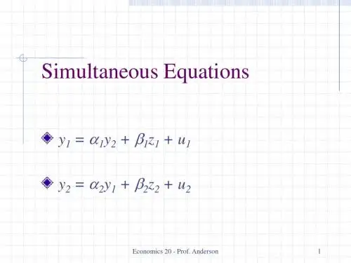
伍德里奇计量经济学导论第六版英文课件Woodridge's Introduction to Econometrics, 6th Edition, is a comprehensive textbook that covers the fundamentals of econometrics in a clear and concise manner. The accompanying courseware is designed to help students further understand and apply the concepts discussed in the book.The courseware includes PowerPoint slides, practice quizzes, and interactive exercises to enhance students' learning experience. The slides cover the key topics in each chapter, providing visual aids to help students grasp complex concepts. The quizzes allow students to test their understanding of the material and receive immediate feedback on their performance. The interactive exercises provide hands-on practice withreal-world data sets, helping students develop their econometric skills.In addition to the courseware, students have access to online resources such as supplementary readings, video tutorials, and self-assessment tools. These resources are designed to support students in their learning journey and provide additional assistance when needed.Overall, Woodridge's Introduction to Econometrics, 6th Edition, is a valuable resource for students studying econometrics. The comprehensive courseware offers a range of tools to support students in their learning, making it easier for them to understand and apply the concepts discussed in the textbook. With its clear explanations and practical exercises, this courseware is an essential companion for students looking to excel in econometrics.。