自适应控制--第二讲 模型参考自适应控制的MIT法
- 格式:ppt
- 大小:1.29 MB
- 文档页数:24

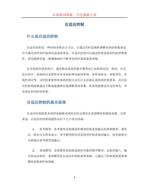
自适应控制什么是自适应控制自适应控制是一种控制系统设计方法,它通过实时监测和调整系统的参数来适应不确定的外部环境和内部系统变化。
自适应控制可以提高控制系统的性能和鲁棒性,使其能够快速、准确地响应不断变化的环境或系统参数。
在传统的控制系统中,通常假设系统的数学模型是已知和固定的。
然而,在实际应用中,系统的动态特性常常受到各种因素的影响,如外部扰动、参数变化、非线性效应等。
这些因素使得传统的控制方法往往无法满足系统的控制要求。
而自适应控制则能够通过不断地观测和在线调整系统参数,使系统能够适应这些变化,并实现良好的控制效果。
自适应控制的基本原理自适应控制的基本原理是根据系统的实时反馈信息来调整控制器的参数。
具体来说,自适应控制系统通常由以下几个部分组成:1.参考模型:参考模型是指描述所期望控制系统输出的理想模型,通常由一组差分方程来表示。
参考模型的作用是指导控制系统的输出,使其能够尽可能接近参考模型的输出。
2.系统模型:系统模型是指描述被控对象的数学模型,包括其输入、输出和动态特性。
系统模型是自适应控制的重要基础,它确定了控制系统需要调整的参数和控制策略。
3.控制器:控制器是自适应控制系统的核心部分,它根据系统输出和参考模型的误差来实时调整控制器的参数。
控制器可以通过不同的算法来实现,如模型参考自适应控制算法、最小二乘自适应控制算法等。
4.参数估计器:参数估计器是自适应控制系统的关键组件,它用于估计系统模型中的未知参数。
参数估计器可以通过不断地观测系统的输入和输出数据来更新参数估计值,从而实现对系统参数的实时估计和调整。
5.反馈环路:反馈环路是指通过测量系统输出并将其与参考模型的输出进行比较,从而产生误差信号并输入到控制器中进行处理。
反馈环路可以帮助控制系统实时调整控制器的参数,使系统能够适应外部环境和内部变化。
自适应控制的应用领域自适应控制在各个领域都有广泛的应用,特别是在复杂和变化的系统中,其优势更为突出。
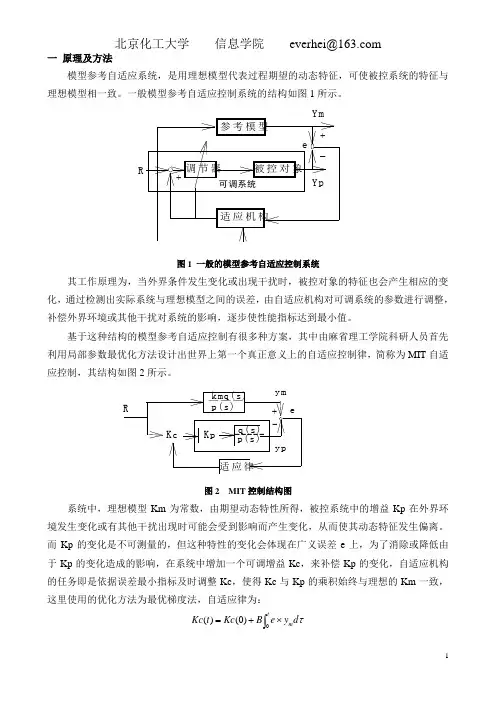
一 原理及方法模型参考自适应系统,是用理想模型代表过程期望的动态特征,可使被控系统的特征与理想模型相一致。
一般模型参考自适应控制系统的结构如图1所示。
图1 一般的模型参考自适应控制系统其工作原理为,当外界条件发生变化或出现干扰时,被控对象的特征也会产生相应的变化,通过检测出实际系统与理想模型之间的误差,由自适应机构对可调系统的参数进行调整,补偿外界环境或其他干扰对系统的影响,逐步使性能指标达到最小值。
基于这种结构的模型参考自适应控制有很多种方案,其中由麻省理工学院科研人员首先利用局部参数最优化方法设计出世界上第一个真正意义上的自适应控制律,简称为MIT 自适应控制,其结构如图2所示。
图2 MIT 控制结构图系统中,理想模型Km 为常数,由期望动态特性所得,被控系统中的增益Kp 在外界环境发生变化或有其他干扰出现时可能会受到影响而产生变化,从而使其动态特征发生偏离。
而Kp 的变化是不可测量的,但这种特性的变化会体现在广义误差e 上,为了消除或降低由于Kp 的变化造成的影响,在系统中增加一个可调增益Kc ,来补偿Kp 的变化,自适应机构的任务即是依据误差最小指标及时调整Kc ,使得Kc 与Kp 的乘积始终与理想的Km 一致,这里使用的优化方法为最优梯度法,自适应律为:⎰⨯+=tm d y e B Kc t Kc 0)0()(τYp Yme+__+R参考模型调节器被控对象适应机构可调系统———kmq(s)p(s)KcKpq(s)-----p(s)适应律Rymype+-MIT 方法的优点在于理论简单,实施方便,动态过程总偏差小,偏差消除的速率快,而且用模拟元件就可以实现;缺点是不能保证过程的稳定性,换言之,被控对象可能会发散。
二 对象及参考模型该实验中我们使用的对象为:122)()()(2++==s s s p s q K s G pp 参考模型为:121)()()(2++==s s s p s q K s G mm 用局部参数最优化方法设计一个模型参考自适应系统,设可调增益的初值Kc(0)=0.2,给定值r(t)为单位阶跃信号,即r(t)=A ×1(t)。

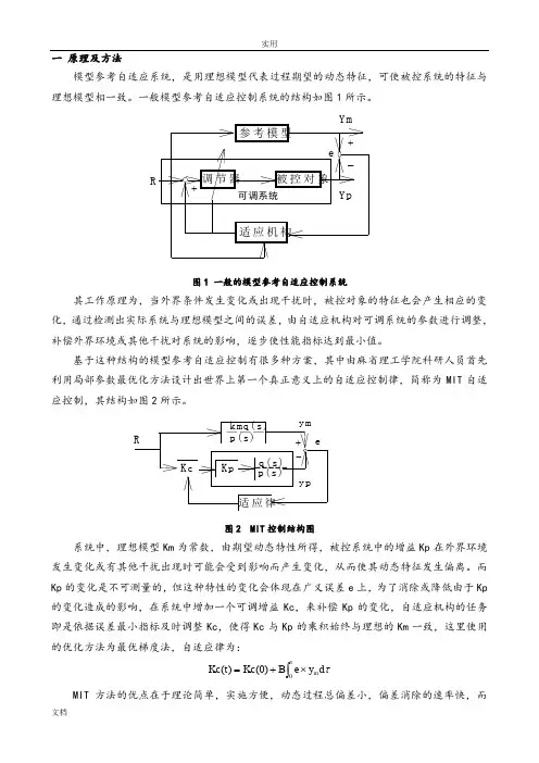
一 原理及方法模型参考自适应系统,是用理想模型代表过程期望的动态特征,可使被控系统的特征与理想模型相一致。
一般模型参考自适应控制系统的结构如图1所示。
图1 一般的模型参考自适应控制系统其工作原理为,当外界条件发生变化或出现干扰时,被控对象的特征也会产生相应的变化,通过检测出实际系统与理想模型之间的误差,由自适应机构对可调系统的参数进行调整,补偿外界环境或其他干扰对系统的影响,逐步使性能指标达到最小值。
基于这种结构的模型参考自适应控制有很多种方案,其中由麻省理工学院科研人员首先利用局部参数最优化方法设计出世界上第一个真正意义上的自适应控制律,简称为MIT 自适应控制,其结构如图2所示。
图2 MIT 控制结构图系统中,理想模型Km 为常数,由期望动态特性所得,被控系统中的增益Kp 在外界环境发生变化或有其他干扰出现时可能会受到影响而产生变化,从而使其动态特征发生偏离。
而Kp 的变化是不可测量的,但这种特性的变化会体现在广义误差e 上,为了消除或降低由于Kp 的变化造成的影响,在系统中增加一个可调增益Kc ,来补偿Kp 的变化,自适应机构的任务即是依据误差最小指标及时调整Kc ,使得Kc 与Kp 的乘积始终与理想的Km 一致,这里使用的优化方法为最优梯度法,自适应律为:⎰⨯+=tm d y e B Kc t Kc 0)0()(τMIT 方法的优点在于理论简单,实施方便,动态过程总偏差小,偏差消除的速率快,而Yp Yme+__+R参考模型调节器被控对象适应机构可调系统———kmq(s)p(s)KcKpq(s)-----p(s)适应律Rymype+-且用模拟元件就可以实现;缺点是不能保证过程的稳定性,换言之,被控对象可能会发散。
二 对象及参考模型该实验中我们使用的对象为:122)()()(2++==s s s p s q K s G pp 参考模型为:121)()()(2++==s s s p s q K s G mm 用局部参数最优化方法设计一个模型参考自适应系统,设可调增益的初值Kc(0)=0.2,给定值r(t)为单位阶跃信号,即r(t)=A ×1(t)。
自适应控制的分类_自适应控制的主要类型什么是自适应控制1、自适应控制所讨论的对象,一般是指对象的结构已知,仅仅是参数未知,而且采用的控制方法仍是基于数学模型的方法。
2、但实践中我们还会遇到结构和参数都未知的对象,比如一些运行机理特别复杂,目前尚未被人们充分理解的对象,不可能建立有效的数学模型,因而无法沿用基于数学模型的方法解决其控制问题,这时需要借助人工智能学科,也就是智能控制。
3、自适应控制与常规的控制与最优控制一样,是一种基于数学模型的控制方法。
4、自适应控制所依据的关于模型的和扰动的先验知识比较少,需要在系统的运行过程中不断提取有关模型的信息,使模型愈来愈准确。
5、常规的反馈控制具有一定的鲁棒性,但是由于控制器参数是固定的,当不确定性很大时,系统的性能会大幅下降,甚至失稳。
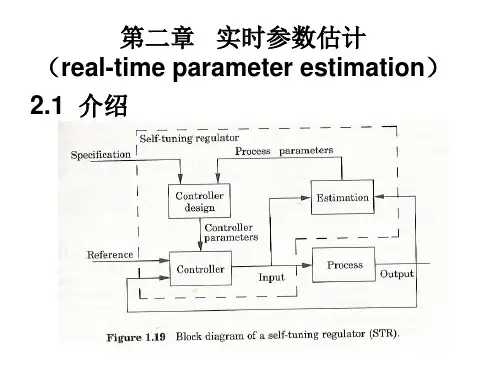
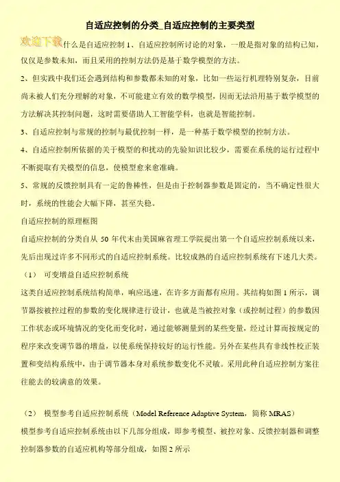
自适应控制的原理框图自适应控制的分类自从50年代末由美国麻省理工学院提出第一个自适应控制系统以来,先后出现过许多不同形式的自适应控制系统。
比较成熟的自适应控制系统有下述几大类。
(1)可变增益自适应控制系统这类自适应控制系统结构简单,响应迅速,在许多方面都有应用。
其结构如图1所示,调节器按被控过程的参数的变化规律进行设计,也就是当被控对象(或控制过程)的参数因工作状态或环境情况的变化而变化时,通过能够测量到的某些变量,经过计算而按规定的程序来改变调节器的增益,以使系统保持较好的运行性能。
另外在某些具有非线性校正装置和变结构系统中,由于调节器本身对系统参数变化不灵敏。
采用此种自适应控制方案往往能去的较满意的效果。
(2)模型参考自适应控制系统(Model Reference Adaptive System,简称MRAS)模型参考自适应控制系统由以下几部分组成,即参考模型、被控对象、反馈控制器和调整控制器参数的自适应机构等部分组成,如图2所示。
自适应控制Adaptive control1.关于控制2.关于自适应控制3.模型参考自适应控制4.自校正控制5.自适应替代方案6.预测控制参考文献主要章节内容说明:第一部分:第一章自适应律的设计§1.参数最优化方法§2.基于Lyapunov稳定性理论的方法§3.超稳定性理论在自适应控制中的应用第二章误差模型§1.Narendra误差模型§2.增广矩阵§3.线性误差模型第三章MRAC的设计和实现第四章小结第二部分:第一章模型辨识及控制器设计§1.系统模型:CARMA模型§2.参数估计:LS法§3.控制器的设计方法:利用传递函数模型§4.自校正第二章最小方差自校正控制§1.最小方差自校正调节器§2.广义最小方差自校正控制第三章极点配置自校正控制§1.间接自校正§2.直接自校正1.About control engineering education1)control curriculum basic concept(1)dynamic system●The processes and plants that are controlled have responses that evolvein time with memory of past responses●The most common mathematical tool used to describe dynamic system isthe ordinary differential equation (ODE).●First approximate the equation as linear and time-invariant. Thenextensions can be made from this foundation that are nonlinear 、time-varying、sampled-data、distributed parameter and so on.●Method of building model (or equation )a)Idea of writing equations of motion based on the physics andchemistry of the situation.b)That of system identification based on experimental data.●Part of understanding the dynamical system requires understanding theperformance limitations and expectation of the system.2.stabilityWith stability, the system can at least be used●Classical control design method, are based on a stability test.Root locus 根轨迹Bode‟s frequency response 波特图Nyquist stability criterion 奈奎斯特判据●Optimal control, especially linear-quadratic Gaussian (LQG) control (线性二次型高斯问题) was always haunted by the fact that method did notinclude a guarantee of margin of stability.The theory and techniques of robust (鲁棒)design have been developedas alternative to LQG●In the realm of nonlinear control, including adaptive control, it iscommon practice to base the design on Lyapunov function in order to beable to guarantee stability of final result.3.feedbackMany open-loop devices such as programmable logic controllers (PLC) are in use, their design and use are not part of control engineering.●The introduction of feedback brings costs as well as benefits. Among thecosts are need for both actuators and sensors, especially sensors.●Actuator defines the control authority and set the limits of speed indynamic response.●Sensor via their inevitable noise, limit the ultimate(最终) accuracy ofcontrol within these limits, feedback affords the benefit of improveddynamic response and stability margins, improved disturbancerejection(拒绝) ,and improved robustness to parameter variability.●The trade off between costs and benefits of feedback is at the center ofcontrol design.4.Dynamic compensation●In beginning there was PID compensation, today remaining a widely usedelement of control, especially in the process control.●Other compensation approaches : lead-and-log networks (超前-滞后)observer-based compensators include : pole placement, LQG designs.●Of increasing interest are designs capable of including trade-off amongstability, dynamic response and parameter robustness.Include: Q parameterization, adaptive schemes.Such as self-tuning regulators, neural-network-based-controllers.二、historical perspectives (透视)●Most of early control manifestations appear as simple on-off (bang-bang)controllers with empirical (实验;经验性的) setting much dependent uponexperience.●The following advances such as Routhis and Hurwitz stability analysis(1877).Lyapunov‟s state model and nonlinear stability criteria(判据) (1890) .Sperry‟s early work on gyroscope and autopilots (1910), and Sikorsky‟swork on ship steering (1923)Take differential equation, Heaviside operators and Laplace transform astheir tools.●电机工程(electrical engineering)The largely changed in the late 1920s and 1930s with Black‟s developmentof the feedback electronic amplifier, Bush‟s differential analyzer, Nyquist‟sstability criterion and Bode‟s frequency response methods.The electrical engineering problems faced usually had vary complex albeitmostly linear model and had arbitrary (独立的;随机的) and wide-ringingdynamics.●过程控制(process control in chemical engineering)Most of the progress controlled were complex and highly nonlinear, butusually had relatively docile (易于处理的) dynamics.One major outcome of this type of work was Ziegler-Nichols‟PIDthres-term controller. This control approach is still in use today, worldwidewith relatively minor modifications and upgrades (including sampled dataPID controllers with feed forward control, anti-integrator-windupcontrollers :抗积分饱和,and fuzzy logic implementations).●机械工程(mechanical engineering)The application of controls in mechanical engineering dealt mostly in thebeginning with mechanism controls, such as servomechanisms, governorsand robots.Some typical control application areas now include manufacturing processcontrols, vehicle dynamic and safety control, biomedical devices and geneticprocess research.Some early methodological outcomes were the olden burger-Kahenbugerdescribing function method of equivalent linearization, and minimum-time,bang-bang control.●航空工程(aeronautical engineering )The problems were generally a hybrid (混合) of well-modeled mechanicsplus marginally understood fluid dynamics. The models were often weaklynonlinear, and the dynamics were sometimes unstable.Major contributions to framework of controls as discipline were Evan‟s rootlocus (1948) and gain-scheduling.●Additional major contributions to growth of the discipline of control over thelast 30-40 years have tended to be independent of traditional disciplines.Examples include:Pontryagin‟s maximum principle (1956) 庞特里金Bellman‟s dynamic programming (1957)贝尔曼Kalman‟s optimal estimation (1960)And the recent advances in robust control.三、Abstract thoughts on curriculum●The possibilities for topic to teach are sufficiently great. If one tries topresent proofs of all theoretical results. One is in danger of giving thestudents many mathematical details with little physical intuition orappreciation for the purposes for which the system is designed.●Control is based on two distinct streams of thought. One stream is physicaland discipline-based. Because one must always be controlling some thing.The other stream is mathematics-based, because the basis concepts ofstability and feedback are fundamentally abstract concepts best expressedmathematically. This duality(两重性) has raised, over the years, regularcomplaints about the …gap‟ between theory and practice.●The control curriculum typically begins with one or two courses designed topresent an overview of control based on linear, constant, ODE models,s-plane and Nyquist‟s stability ideas, SISO feedback and PID, lead-lay andpole-placement compensation.These introductory courses can then be followed by courses in linear systemtheory, digital of control, optimal control, advanced theory of feedback, andsystem identification.四、Main control courses●Introduction to controlLumped system theoryNonlinear controlOptimal controlAdaptive controlRobot controlDigital controlModeling and simulationAdvanced theoryStochastic processesLarge scale multivariable systemManufacturing systemFuzzy logic Neural Networks外文期刊:《Automatic》IFAC 国际自动控制联合会Computer and control abstractsIEEE translations on Automatic controlAutomation●Specialized \ experimental courses✓Intelligent controlApplication of Artificial IntelligenceSimulation and optimization of lager scale systems robust control ✓System identification✓Microcomputer-based control systemDiscrete-event systemsParallel and Distributed computationNumerical optimization methodsNumerical system theory●Top key works from 1963-1995 in IIACAdaptive control 305Optimal control 277Identification 255Parameter estimation 244Stability 217Linear system 184Non-linear systems 168Robust control 158Discrete-time systems 143Multivariable systems 140Robustness 140Multivariable systems control systems 110Optimization 110Computer control 104Large-scale systems 103Kalman filter 102Modeling 107为什么自适应 《Astrom 》chapter 1✓ 反馈可以消除扰动。