线性规划的灵敏度分析实验报告
- 格式:doc
- 大小:105.00 KB
- 文档页数:27
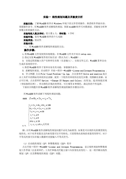
实验一 线性规划问题及灵敏度分析实验目的:了解WinQSB 软件在Windows 环境下的文件管理操作,熟悉软件界面内容,掌握操作命令。
用WinQSB 软件求解线性规划,掌握winQSB 软件写对偶规划,灵敏度分析和参数分析的操作方法。
实验每组人数及学时:组人数1人,学时数:4学时 实验环境:装有WinQSB 软件的个人电脑 实验类型:验证性 实验内容:一、 用WinQSB 软件求解线性规划的方法:操作步骤:1.将WinQSB 文件复制到本地硬盘;在WinQSB 文件夹中双击setup.exe 。
2.指定安装WinQSB 软件的目标目录(默认为C:\ WinQSB )。
3. 安装过程需输入用户名和单位名称(任意输入),安装完毕之后,WinQSB 菜单自动生成在系统程序中。
4.熟悉WinQSB 软件子菜单内容及其功能,掌握操作命令。
5.求解线性规划。
启动程序 开始→程序→WinQSB→Linear and Integer Programming 。
6.学习例题 点击File→Load Problem→lp.lpp, 点击菜单栏Solve and Analyze 或点击工具栏中的图标用单纯形法求解,观赏一下软件用单纯形法迭代步骤。
用图解法求解,显示可行域,点击菜单栏Option →Change XY Ranges and Colors,改变X1、X2的取值区域(坐标轴的比例),单击颜色区域改变背景、可行域等8种颜色,满足你的个性选择。
下面结合例题介绍WinQSB 软件求解线性规划的操作步骤及应用。
用WinQSB 软件求解下列线性规划问题:1234max 657Z x x x x =+++s.t. 12341234123123431234269260852150730001020,,0,x x x x x x x x x x x x x x x x x x x x +++≤⎧⎪-+-≥⎪⎪++=⎪-≥⎨⎪-≥⎪≤≤⎪⎪≥⎩无约束解:应用WinQSB 软件求解线性规划问题不必化为标准型,如果是可以线性化的模型则先线性化,对于有界变量及无约束变量可以不用转化,只需要修改系统的变量类型即可,对于不等式约束可以在输入数据时直接输入不等式符号。
实验3 线性规划的灵敏性分析专业班级信息121 班学号201212030120 姓名刘帅报告日期实验类型:●验证性实验○综合性实验○设计性实验实验目的:熟练线性规划图解法的灵敏性分析。
实验内容:线性规划的灵敏性分析4个(题目自选b,c灵敏性分析)实验原理在线性规划图解法求出最优解的情况下,分析b,c分别变化对最优解的影响,确定最优解的变化范围,在变化的情况下能求出最优解。
实验步骤1 要求上机实验前先编写出程序代码2 编辑录入程序3 调试程序并记录调试过程中出现的问题及修改程序的过程4 经反复调试后,运行程序并验证程序运行是否正确。
5 记录运行时的输入和输出。
预习编写程序代码:实验报告:根据实验情况和结果撰写并递交实验报告。
(1) 唯一最优解:max z=x1+x2⎪⎩⎪⎨⎧≥≤+≤+02,182126221X X X X X X建立simplex.m 文件function [x,z,flg,sgma]=simplex(A,A1,b,c,m,n,n1,cb,xx)% A,b are the matric in A*x=b% c is the matrix in max z=c*x% A1 is the matric in simplex table% m is the numbers of row in A and n is the column number in A% n1 is the nubers of artificial variables,and artificial variables are default at the last % n1 variables in x.% cb is the worth coefficient matrix for basic variables% xx is the index matrix for basic variables% B1 is the invers matrix for the basic matrix in simplex table.The initial % matrix is default as the last m con in the matrix A.x=zeros(n,1)。

线性规划实验报告线性规划实验报告1.路径规划问题第一步:在excel表格中建立如下表格,详细列名各节点路线及其权重。
起点终点权数0-1 节点进出和V1 V2 5 V1 1V1 V3 2 V2 0V2 V4 2 V3 0V2 V5 7 V4 0V3 V4 7 V5 0V3 V6 4 V6 0V4 V5 6 V7 -1V4 V6 2V5 V6 1V5 V7 3V6 V7 6 目标第二步:在进出和一列以公式表示各节点的进出流量和。
V1=V12+V13;V2=V24+V25-V12;V3=V34+V36-V13;V4=V45+V46-V24-V34;V5=V56+V57-V25-V45;V6=V67-V36-V46-V56V7=-V57-V67.第三步:设置目标函数为SUMPRODUCT(C2:C12,D2:D12)第四步:设置可变单元格和限制条件。
选定0-1一列,D2:D12为可变单元格。
可变单元格数值介于0-1之间,且为整数。
进出和数值与设定值相等。
第五步:规划求解,结果如下。
由表可知,从V1至V7的最短路径为V1——V3——V6——V7,最小目标值为12。
起点终点权重0-1 节点进出和V1 V2 5 0 V1 1 = 1 V1 V3 2 1 V2 0 = 0 V2 V4 2 0 V3 0 = 0 V2 V5 7 0 V4 0 = 0 V3 V4 7 0 V5 0 = 0 V3 V6 4 1 V6 0 = 0 V4 V5 6 0 V7 -1 = -1 V4 V6 2 0V5 V6 1 0V5 V7 3 0V6 V7 6 1 目标函数12Microsoft Excel 11.0 运算结果报告工作表 [复件 11.xls]Sheet2报告的建立: 2013-12-12 14:07:00目标单元格 (最小值)单元格名字初值终值$F$12 目标函数进出和12 12可变单元格单元格名字初值终值$D$2 V2 0-1 2.22E-16 0$D$3 V3 0-1 1 1$D$4 V4 0-1 0 0$D$5 V5 0-1 2.22045E-16 0$D$6 V4 0-1 0 0$D$7 V6 0-1 1 1$D$8 V5 0-1 0 0$D$9 V6 0-1 0 0$D$10 V6 0-1 0 0$D$11 V7 0-1 2.22045E-16 0$D$12 V7 0-1 1 1约束单元格名字单元格值公式状态型数值$F$2 V1 进出和 1 $F$2=$I$2 未到限制值$F$3 V2 进出和0 $F$3=$I$3 未到限制值$F$4 V3 进出和0 $F$4=$I$4 未到限制值$F$5 V4 进出和0 $F$5=$I$5 未到限制值$F$6 V5 进出和0 $F$6=$I$6 未到限制值$F$7 V6 进出和0 $F$7=$I$7 未到限制值$F$8 V7 进出和-1 $F$8=$I$8 未到限制值$D$2 V2 0-1 0 $D$2<=1 未到限制值1$D$3 V3 0-1 1 $D$3<=1 到达限制值$D$4 V4 0-1 0 $D$4<=1 未到限制值1$D$5 V5 0-1 0 $D$5<=1 未到限制值1$D$6 V4 0-1 0 $D$6<=1 未到限制值1$D$7 V6 0-1 1 $D$7<=1 到达限制值$D$8 V5 0-1 0 $D$8<=1 未到限制值1$D$9 V6 0-1 0 $D$9<=1 未到限制值1$D$10 V6 0-1 0 $D$10<=1 未到限制值1$D$11 V7 0-1 0 $D$11<=1 未到限制值1$D$12 V7 0-1 1 $D$12<=1 到达限制值$D$2 V2 0-1 0 $D$2>=0 到达限制值$D$3 V3 0-1 1 $D$3>=0 未到限制值1$D$4 V4 0-1 0 $D$4>=0 到达限制值$D$5 V5 0-1 0 $D$5>=0 到达限制$D$6 V4 0-1 0 $D$6>=0 到达限制值$D$7 V6 0-1 1 $D$7>=0 未到限制值1$D$8 V5 0-1 0 $D$8>=0 到达限制值$D$9 V6 0-1 0 $D$9>=0 到达限制值$D$10 V6 0-1 0 $D$10>=0 到达限制值$D$11 V7 0-1 0 $D$11>=0 到达限制值$D$12 V7 0-1 1 $D$12>=0 未到限制值1$D$2 V2 0-1 0 $D$2=整数到达限制值$D$3 V3 0-1 1 $D$3=整数到达限制值$D$4 V4 0-1 0 $D$4=整数到达限制值$D$5 V5 0-1 0 $D$5=整数到达限制值$D$6 V4 0-1 0 $D$6=整数到达限制值$D$7 V6 0-1 1 $D$7=整数到达限制值$D$8 V5 0-1 0 $D$8=整数到达限制$D$9 V6 0-1 0 $D$9=整数到达限制值$D$10 V6 0-1 0 $D$10=整数到达限制值$D$11 V7 0-1 0 $D$11=整数到达限制值$D$12 V7 0-1 1 $D$12=整数到达限制值2.运用Excel构建线性规划模型与求解实验报告一、实验目的1.掌握线性规划问题建模基本方法。


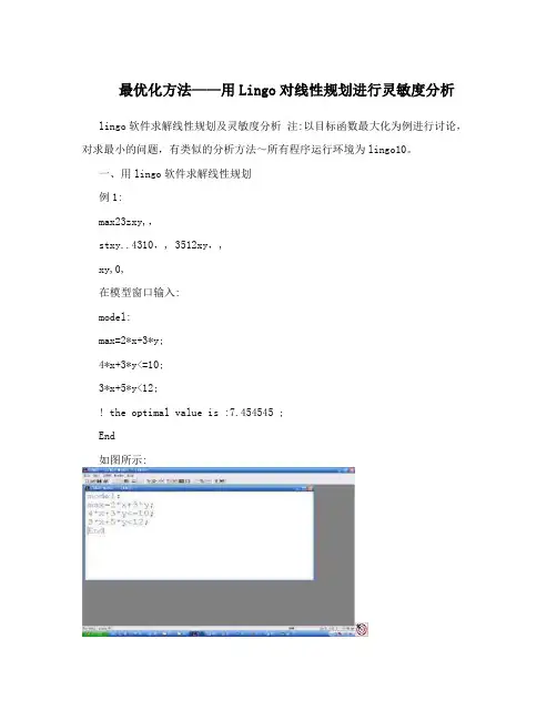
最优化方法——用Lingo对线性规划进行灵敏度分析lingo软件求解线性规划及灵敏度分析注:以目标函数最大化为例进行讨论,对求最小的问题,有类似的分析方法~所有程序运行环境为lingo10。
一、用lingo软件求解线性规划例1:max23zxy,,stxy..4310,, 3512xy,,xy,0,在模型窗口输入:model:max=2*x+3*y;4*x+3*y<=10;3*x+5*y<12;! the optimal value is :7.454545 ;End如图所示:运行结果如下(点击工具栏上的‘solve’或点击菜单‘lingo’下的‘solve’即可):Global optimal solution found.Objective value: 7.454545(最优解函数值)Total solver iterations: 2(迭代次数)1Variable (最优解) Value Reduced CostX 1.272727 0.000000Y 1.636364 0.000000Row Slack or Surplus Dual Price1 7.454545 1.0000002 0.000000 0.9090909E-013 0.000000 0.5454545 例2:max54zxx,,12stxxx..390,,,123280xxx,,,124xxx,,,45125x,0在模型窗口输入:model:max=5*x1+4*x2;x1+3*x2+x3=90;2*x1+x2+x4=80;x1+x2+x5=45;end运行(solve)结果如下:Global optimal solution found. Objective value: 215.0000Total solver iterations: 3 Variable Value Reduced CostX1 35.00000 0.000000X2 10.00000 0.000000X3 25.00000 0.000000X4 0.000000 1.000000X5 0.000000 3.000000Row Slack or Surplus Dual Price1 215.0000 1.0000002 0.000000 0.0000003 0.000000 1.0000004 0.000000 3.000000例32min2zxx,,,23stxxx..22,,,123xxx,,,31234xxx,,,2235x,0在模型窗口输入:model:min=-x2+2*x3;x1-2*x2+x3=2;x2-3*x3+x4=1;x2-x3+x5=2;end运行结果如下:Global optimal solution found. Objective value: -1.500000 Total solver iterations: 2 Variable Value Reduced CostX2 2.500000 0.000000X3 0.5000000 0.000000X1 6.500000 0.000000X4 0.000000 0.5000000X5 0.000000 0.5000000Row Slack or Surplus Dual Price1 -1.500000 -1.0000002 0.000000 0.0000003 0.000000 0.50000004 0.000000 0.5000000 例4: minxyz,,stxy..1,,24xz,,在模型窗口输入:model:min=@abs(x)+@abs(y)+@abs(z);x+y<1;2*x+z=4;@free(x);@free(y);@free(z);3End求解器状态如下:(可看出是非线性模型~)运行结果为:Linearization components added: Constraints: 12Variables: 12Integers: 3Global optimal solution found.Objective value: 3.000000Extended solver steps: 0Total solver iterations: 4Variable Value Reduced CostX 2.000000 0.000000Y -1.000000 0.000000Z 0.000000 0.000000Row Slack or Surplus Dual Price1 3.000000 -1.0000002 0.000000 1.0000003 0.000000 -1.000000 二、用lingo软件进行灵敏度分析实例例5:4max603020Sxyz,,,8648xyz,,,421.520xyz,,, 21.50.58xyz,,,y,5xyz,,0,在模型窗口输入:Lingo模型:model:max=60*x+30*y+20*z;8*x+6*y+z<48;4*x+2*y+1.5*z<20;2*x+1.5*y+0.5*z<8;y<5;end(一)求解报告(solution report)通过菜单Lingo?Solve可以得到求解报告(solution report)如下:Global optimal solution found at iteration: 0Objective value: 280.0000Variable Value Reduced CostX 2.000000 0.000000Y 0.000000 5.000000Z 8.000000 0.000000Row Slack or Surplus Dual Price1 280.0000 1.0000002 24.00000 0.0000003 0.000000 10.000004 0.000000 10.000005 5.000000 0.000000 分析Value,Reduced Cost,Slack or Surplus,Dual Price的意义如下: 1、最优解和基变量的确定Value所在列给出了问题的最优解。

lingo 软件求解线性规划及灵敏度分析注:以目标函数最大化为例进行讨论,对求最小的问题,有类似的分析方法!所有程序运行环境为lingo10。
一、用lingo 软件求解线性规划例1:max 23..43103512,0z x y s t x y x y x y =++≤+≤≥在模型窗口输入:model: max=2*x+3*y; 4*x+3*y<=10; 3*x+5*y<12;! the optimal value is :7.454545 ; End 如图所示:运行结果如下(点击 工具栏上的‘solve ’或点击菜单‘lingo ’下的‘solve ’即可):Global optimal solution found.Objective value: 7.454545(最优解函数值) Total solver iterations: 2(迭代次数)Variable (最优解) Value Reduced Cost X 1.272727 0.000000 Y 1.636364 0.000000Row Slack or Surplus Dual Price 1 7.454545 1.000000 2 0.000000 0.9090909E-01 3 0.000000 0.5454545例2:12123124125max 54..390280450z x x s t x x x x x x x x x x =+++=++=++=≥ 在模型窗口输入:model:max=5*x1+4*x2; x1+3*x2+x3=90; 2*x1+x2+x4=80; x1+x2+x5=45; end运行(solve )结果如下:Global optimal solution found.Objective value: 215.0000 Total solver iterations: 3Variable Value Reduced Cost X1 35.00000 0.000000 X2 10.00000 0.000000 X3 25.00000 0.000000 X4 0.000000 1.000000 X5 0.000000 3.000000Row Slack or Surplus Dual Price 1 215.0000 1.000000 2 0.000000 0.000000 3 0.000000 1.000000 4 0.000000 3.000000例323123234235min 2..223120z x x s t x x x x x x x x x x =-+-+=-+=-+=≥ 在模型窗口输入:model:min=-x2+2*x3; x1-2*x2+x3=2; x2-3*x3+x4=1; x2-x3+x5=2; end运行结果如下:Global optimal solution found.Objective value: -1.500000 Total solver iterations: 2Variable Value Reduced Cost X2 2.500000 0.000000 X3 0.5000000 0.000000 X1 6.500000 0.000000 X4 0.000000 0.5000000 X5 0.000000 0.5000000Row Slack or Surplus Dual Price 1 -1.500000 -1.000000 2 0.000000 0.000000 3 0.000000 0.5000000 4 0.000000 0.5000000例4:min ..124x y z s t x y x z +++≤+= 在模型窗口输入:model :min =@abs (x)+@abs (y)+@abs (z); x+y<1; 2*x+z=4; @free (x); @free (y); @free (z);End求解器状态如下:(可看出是非线性模型!)运行结果为:Linearization components added:Constraints: 12Variables: 12Integers: 3Global optimal solution found.Objective value: 3.000000Extended solver steps: 0Total solver iterations: 4Variable Value Reduced Cost X 2.000000 0.000000Y -1.000000 0.000000 Z 0.000000 0.000000Row Slack or Surplus Dual Price1 3.000000 -1.0000002 0.000000 1.0000003 0.000000 -1.000000二、用lingo软件进行灵敏度分析实例例5:max 603020864842 1.5202 1.50.585,,0S x y z x y z x y z x y z y x y z =++++≤++≤++≤≤≥在模型窗口输入: Lingo 模型:model:max=60*x+30*y+20*z; 8*x+6*y+z<48; 4*x+2*y+1.5*z<20; 2*x+1.5*y+0.5*z<8; y<5; end(一)求解报告(solution report )通过菜单Lingo →Solve 可以得到求解报告(solution report )如下:Global optimal solution found at iteration: 0 Objective value: 280.0000Variable Value Reduced Cost X 2.000000 0.000000 Y 0.000000 5.000000 Z 8.000000 0.000000Row Slack or Surplus Dual Price 1 280.0000 1.000000 2 24.00000 0.000000 3 0.000000 10.00000 4 0.000000 10.00000 5 5.000000 0.000000分析Value,Reduced Cost ,Slack or Surplus ,Dual Price 的意义如下: 1、最优解和基变量的确定Value 所在列给出了问题的最优解。
最优化方法——用Lingo对线性规划进行灵敏度分析lingo软件求解线性规划及灵敏度分析注:以目标函数最大化为例进行讨论,对求最小的问题,有类似的分析方法~所有程序运行环境为lingo10。
一、用lingo软件求解线性规划例1:max23zxy,,stxy..4310,, 3512xy,,xy,0,在模型窗口输入:model:max=2*x+3*y;4*x+3*y<=10;3*x+5*y<12;! the optimal value is :7.454545 ; End如图所示:运行结果如下(点击工具栏上的‘solve’或点击菜单‘lingo’下的‘solve’即可):Global optimal solution found.Objective value: 7.454545(最优解函数值)Total solver iterations: 2(迭代次数)road, are the structural road traffic within the city. In addition, suitable for high speed, and high-speed, S206, S307, also serve inner-city traffic. Outbound traffic: existing highways (suitable for high-speed, and high speed), darts (S206, S307) and Yi wei road, and so on. After years of constant development, road conditions have been greatly Variable (最优解) Value Reduced CostX 1.272727 0.000000Y 1.636364 0.000000Row Slack or Surplus Dual Price1 7.454545 1.0000002 0.000000 0.9090909E-013 0.000000 0.5454545 例2:max54zxx,,12stxxx..390,,,123280xxx,,,124xxx,,,45125x,0在模型窗口输入:model:max=5*x1+4*x2;x1+3*x2+x3=90;2*x1+x2+x4=80;x1+x2+x5=45;end运行(solve)结果如下:Global optimal solution found.Objective value: 215.0000Total solver iterations: 3Variable Value Reduced CostX1 35.00000 0.000000X2 10.00000 0.000000X3 25.00000 0.000000X4 0.000000 1.000000X5 0.000000 3.000000Row Slack or Surplus Dual Price1 215.0000 1.0000002 0.000000 0.0000003 0.000000 1.0000004 0.000000 3.000000例3conditions have been greatly speed, and high speed), darts (S206, S307) and Yi wei road, and so on. After years of constant development, road-city traffic. Outbound traffic: existing highways (suitable forhigh-speed, S206, S307, also serve inner-ion, suitable for high speed, and highroad, are the structural road traffic within the city. In addit2 min2zxx,,,23stxxx..22,,,123xxx,,,31234xxx,,,2235x,0在模型窗口输入:model:min=-x2+2*x3;x1-2*x2+x3=2;x2-3*x3+x4=1;x2-x3+x5=2;end运行结果如下:Global optimal solution found.Objective value: -1.500000Total solver iterations: 2Variable Value Reduced CostX2 2.500000 0.000000X3 0.5000000 0.000000X1 6.500000 0.000000X4 0.000000 0.5000000X5 0.000000 0.5000000Row Slack or Surplus Dual Price1 -1.500000 -1.0000002 0.000000 0.0000003 0.000000 0.50000004 0.000000 0.5000000 例4:minxyz,,stxy..1,,24xz,,在模型窗口输入:model:min=@abs(x)+@abs(y)+@abs(z);x+y<1;2*x+z=4;@free(x);@free(y);@free(z);greatly nd high speed), darts (S206, S307) and Yi wei road, and so on. After years of constant development, road conditions have beenspeed, a-city traffic. Outbound traffic: existing highways (suitable for high-speed, S206, S307, also serve inner-road, are the structural roadtraffic within the city. In addition, suitable for high speed, and high3 End求解器状态如下:(可看出是非线性模型~)运行结果为:Linearization components added: Constraints: 12Variables: 12Integers: 3Global optimal solution found. Objective value: 3.000000 Extended solver steps: 0Total solver iterations: 4 Variable Value Reduced CostX 2.000000 0.000000Y -1.000000 0.000000Z 0.000000 0.000000Row Slack or Surplus Dual Price1 3.000000 -1.0000002 0.000000 1.0000003 0.000000 -1.000000二、用lingo软件进行灵敏度分析实例例5:conditions have been greatly speed, and high speed), darts (S206,S307) and Yi wei road, and so on. After years of constant development, road-city traffic. Outbound traffic: existing highways (suitable forhigh-speed, S206, S307, also serve inner-ion, suitable for high speed, and highroad, are the structural road traffic within the city. In addit4 max603020Sxyz,,,8648xyz,,,421.520xyz,,, 21.50.58xyz,,,y,5xyz,,0,在模型窗口输入:Lingo模型:model:max=60*x+30*y+20*z;8*x+6*y+z<48;4*x+2*y+1.5*z<20;2*x+1.5*y+0.5*z<8;y<5;end(一)求解报告(solution report)通过菜单Lingo?Solve可以得到求解报告(solution report)如下:Global optimal solution found at iteration: 0Objective value: 280.0000Variable Value Reduced CostX 2.000000 0.000000Y 0.000000 5.000000Z 8.000000 0.000000Row Slack or Surplus Dual Price1 280.0000 1.0000002 24.00000 0.0000003 0.000000 10.000004 0.000000 10.000005 5.000000 0.000000分析Value,Reduced Cost,Slack or Surplus,Dual Price的意义如下: 1、最优解和基变量的确定Value所在列给出了问题的最优解。
. . . . .. . c. .. .. . 《运筹学/线性规划》实验报告
实验室: 实验日期: 实验项目 线性规划的灵敏度分析 系 别 数学系
姓 名 学 号 班 级 指导教师 成 绩 . . . . .. .
c. .. .. . 一 实验目的 掌握用Lingo/Lindo对线性规划问题进行灵敏度分析的方法,理解解报告的内容。初
步掌握对实际的线性规划问题建立数学模型,并利用计算机求解分析的一般方法。
二 实验环境 Lingo软件
三 实验内容(包括数学模型、上机程序、实验结果、结果分析与问题解答等) 例题2-10 MODEL: [_1] MAX= 2 * X_1 + 3 * X_2 ; [_2] X_1 + 2 * X_2 + X_3 = 8 ; [_3] 4 * X_1 + X_4 = 16 ; [_4] 4 * X_2 + X_5 = 12 ; END 编程 sets: is/1..3/:b; js/1..5/:c,x; links(is,js):a; endsets max=sum(js(J):c(J)*x(J)); for(is(I):sum(js(J):a(I,J)*x(J))=b(I)); data: c=2 3 0 0 0; b=8 16 12; a=1 2 1 0 0 4 0 0 1 0 0 4 0 0 1; end data end
灵敏度分析 Ranges in which the basis is unchanged: . . . . .. . c. .. .. . Objective Coefficient Ranges Current Allowable Allowable Variable Coefficient Increase Decrease X( 1) 2.000000 INFINITY 0.5000000 X( 2) 3.000000 1.000000 3.000000 X( 3) 0.0 1.500000 INFINITY X( 4) 0.0 0.1250000 INFINITY X( 5) 0.0 0.7500000 0.2500000
Righthand Side Ranges Row Current Allowable Allowable RHS Increase Decrease 2 8.000000 2.000000 4.000000 3 16.00000 16.00000 8.000000 4 12.00000 INFINITY 4.000000 当b2在 [8,32]之间变化时 最优基不变
最优解 Global optimal solution found at iteration: 0 Objective value: 14.00000 Variable Value Reduced Cost B( 1) 8.000000 0.000000 B( 2) 16.00000 0.000000 B( 3) 12.00000 0.000000 C( 1) 2.000000 0.000000 C( 2) 3.000000 0.000000 C( 3) 0.000000 0.000000 C( 4) 0.000000 0.000000 C( 5) 0.000000 0.000000 X( 1) 4.000000 0.000000 X( 2) 2.000000 0.000000 X( 3) 0.000000 1.500000 X( 4) 0.000000 0.1250000 X( 5) 4.000000 0.000000 A( 1, 1) 1.000000 0.000000 . . . . .. . c. .. .. . A( 1, 2) 2.000000 0.000000 A( 1, 3) 1.000000 0.000000 A( 1, 4) 0.000000 0.000000 A( 1, 5) 0.000000 0.000000 A( 2, 1) 4.000000 0.000000 A( 2, 2) 0.000000 0.000000 A( 2, 3) 0.000000 0.000000 A( 2, 4) 1.000000 0.000000 A( 2, 5) 0.000000 0.000000 A( 3, 1) 0.000000 0.000000 A( 3, 2) 4.000000 0.000000 A( 3, 3) 0.000000 0.000000 A( 3, 4) 0.000000 0.000000 A( 3, 5) 1.000000 0.000000
Row Slack or Surplus Dual Price 1 14.00000 1.000000 2 0.000000 1.500000 3 0.000000 0.1250000 4 0.000000 0.000000
例题2-11 模型 MAX 2 X( 1) + 3 X( 2) SUBJECT TO 2] X( 1) + 2 X( 2) + X( 3) = 12 3] 4 X( 1) + X( 4) = 16 4] 4 X( 2) + X( 5) = 12 END
编程 sets: is/1..3/:b; js/1..5/:c,x; links(is,js):a; . . . . .. . c. .. .. . endsets max=sum(js(J):c(J)*x(J)); for(is(I):sum(js(J):a(I,J)*x(J))=b(I)); data: c=2 3 0 0 0; b=12 16 12; a=1 2 1 0 0 4 0 0 1 0 0 4 0 0 1; end data end
最优解 Global optimal solution found at iteration: 2 Objective value: 17.00000 Variable Value Reduced Cost B( 1) 12.00000 0.000000 B( 2) 16.00000 0.000000 B( 3) 12.00000 0.000000 C( 1) 2.000000 0.000000 C( 2) 3.000000 0.000000 C( 3) 0.000000 0.000000 C( 4) 0.000000 0.000000 C( 5) 0.000000 0.000000 X( 1) 4.000000 0.000000 X( 2) 3.000000 0.000000 X( 3) 2.000000 0.000000 X( 4) 0.000000 0.5000000 X( 5) 0.000000 0.7500000 A( 1, 1) 1.000000 0.000000 A( 1, 2) 2.000000 0.000000 A( 1, 3) 1.000000 0.000000 A( 1, 4) 0.000000 0.000000 A( 1, 5) 0.000000 0.000000 A( 2, 1) 4.000000 0.000000 . . . . .. . c. .. .. . A( 2, 2) 0.000000 0.000000 A( 2, 3) 0.000000 0.000000 A( 2, 4) 1.000000 0.000000 A( 2, 5) 0.000000 0.000000 A( 3, 1) 0.000000 0.000000 A( 3, 2) 4.000000 0.000000 A( 3, 3) 0.000000 0.000000 A( 3, 4) 0.000000 0.000000 A( 3, 5) 1.000000 0.000000
Row Slack or Surplus Dual Price 1 17.00000 1.000000 2 0.000000 0.000000 3 0.000000 0.5000000 4 0.000000 0.7500000
最优解(4,3,2,0,0)最优值z=17 分析 Ranges in which the basis is unchanged:
Objective Coefficient Ranges Current Allowable Allowable Variable Coefficient Increase Decrease X( 1) 2.000000 INFINITY 2.000000 X( 2) 3.000000 INFINITY 3.000000 X( 3) 0.0 1.500000 INFINITY X( 4) 0.0 0.5000000 INFINITY X( 5) 0.0 0.7500000 INFINITY
Righthand Side Ranges Row Current Allowable Allowable RHS Increase Decrease 2 12.00000 INFINITY 2.000000 3 16.00000 8.000000 16.00000 4 12.00000 4.000000 12.00000