伍德里奇计量经济学第六版答案Chapter-3
- 格式:pdf
- 大小:468.10 KB
- 文档页数:15
伍德里奇《计量经济学导论》(第6版)复习笔记和课后习题详解OLS用于时间序列数据的其他问题第11章OLS用于时间序列数据的其他问题11.1复习笔记考点一:平稳和弱相关时间序列★★★★1.时间序列的相关概念(见表11-1)表11-1时间序列的相关概念2.弱相关时间序列(1)弱相关对于一个平稳时间序列过程{x t:t=1,2,…},随着h的无限增大,若x t和x t+h“近乎独立”,则称为弱相关。
对于协方差平稳序列,如果x t和x t+h之间的相关系数随h的增大而趋近于0,则协方差平稳随机序列就是弱相关的。
本质上,弱相关时间序列取代了能使大数定律(LLN)和中心极限定理(CLT)成立的随机抽样假定。
(2)弱相关时间序列的例子(见表11-2)表11-2弱相关时间序列的例子考点二:OLS的渐近性质★★★★1.OLS的渐近性假设(见表11-3)表11-3OLS的渐近性假设2.OLS的渐近性质(见表11-4)表11-4OLS的渐进性质考点三:回归分析中使用高度持续性时间序列★★★★1.高度持续性时间序列(1)随机游走(见表11-5)表11-5随机游走(2)带漂移的随机游走带漂移的随机游走的形式为:y t=α0+y t-1+e t,t=1,2,…。
其中,e t(t=1,2,…)和y0满足随机游走模型的同样性质;参数α0被称为漂移项。
通过反复迭代,发现y t的期望值具有一种线性时间趋势:y t=α0t+e t+e t-1+…+e1+y0。
当y0=0时,E(y t)=α0t。
若α0>0,y t的期望值随时间而递增;若α0<0,则随时间而下降。
在t时期,对y t+h的最佳预测值等于y t加漂移项α0h。
y t的方差与纯粹随机游走情况下的方差完全相同。
带漂移随机游走是单位根过程的另一个例子,因为它是含截距的AR(1)模型中ρ1=1的特例:y t=α0+ρ1y t-1+e t。
2.高度持续性时间序列的变换(1)差分平稳过程I(1)弱相关过程,也被称为0阶单整或I(0),这种序列的均值已经满足标准的极限定理,在回归分析中使用时无须进行任何处理。

第三篇高级专题第13章跨时横截面的混合:简单面板数据方法13.1 复习笔记考点一:跨时独立横截面的混合★★★★★1.独立混合横截面数据的定义独立混合横截面数据是指在不同时点从一个大总体中随机抽样得到的随机样本。
这种数据的重要特征在于:都是由独立抽取的观测所构成的。
在保持其他条件不变时,该数据排除了不同观测误差项的相关性。
区别于单独的随机样本,当在不同时点上进行抽样时,样本的性质可能与时间相关,从而导致观测点不再是同分布的。
2.使用独立混合横截面的理由(见表13-1)表13-1 使用独立混合横截面的理由3.对跨时结构性变化的邹至庄检验(1)用邹至庄检验来检验多元回归函数在两组数据之间是否存在差别(见表13-2)表13-2 用邹至庄检验来检验多元回归函数在两组数据之间是否存在差别(2)对多个时期计算邹至庄检验统计量的办法①使用所有时期虚拟变量与一个(或几个、所有)解释变量的交互项,并检验这些交互项的联合显著性,一般总能检验斜率系数的恒定性。
②做一个容许不同时期有不同截距的混合回归来估计约束模型,得到SSR r。
然后,对T个时期都分别做一个回归,并得到相应的残差平方和,有:SSR ur=SSR1+SSR2+…+SSR T。
若有k个解释变量(不包括截距和时期虚拟变量)和T个时期,则需检验(T-1)k 个约束。
而无约束模型中有T+Tk个待估计参数。
所以,F检验的df为(T-1)k和n-T -Tk,其中n为总观测次数。
F统计量计算公式为:[(SSR r-SSR ur)/SSR ur][(n-T-Tk)/(Tk-k)]。
但该检验不能对异方差性保持稳健,为了得到异方差-稳健的检验,必须构造交互项并做一个混合回归。
4.利用混合横截面作政策分析(1)自然实验与真实实验当某些外生事件改变了个人、家庭、企业或城市运行的环境时,便产生了自然实验(准实验)。
一个自然实验总有一个不受政策变化影响的对照组和一个受政策变化影响的处理组。

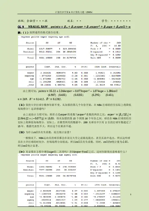
班级:金融学×××班姓名:××学号:×××××××C6.9 NBASAL.RAW points=β0+β1exper+β2exper2+β3age+β4coll+u 解:(ⅰ)按照通常的格式报告结果。
由上图可知:points=35.22+2.364exper−0.077exper2−1.074age−1.286coll6.9870.4050.02350.295 (0.451)n=269,R2=0.1412,R2=0.1282。
(ⅱ)保持大学打球年数和年龄不变,从加盟的第几个年份开始,在NBA打球的经历实际上将降低每场得分?这讲得通吗?由上述估计方程可知,转折点是exper的系数与exper2系数的两倍之比:exper∗= β12β2= 2.364[2×−0.077]=15.35,即从加盟的第15个到第16个年份之间,球员在NBA打球的经历实际上将降低每场得分。
实际上,在模型所用的数据中,269名球员中只有2位的打球年数超过了15年,数据代表性不大,所以这个结果讲不通。
(ⅲ)为什么coll具有负系数,而且统计显著?一般情况下,NBA运动员的球员都会在读完大学之前被选拔出,甚至从高中选出,所以这些球员在大学打球的时间少,但每场得分却很高,所以coll具有负系数。
同时,coll的t统计量为-2.85,所以coll统计显著。
(ⅳ)有必要在方程中增加age的二次项吗?控制exper和coll之后,这对年龄效应意味着什么?增加age的二次项后,原估计模型变成:points=73.59+2.864exper−0.128exper2−3.984age+0.054age2−1.313coll35.930.610.05 2.690.05 (0.45)n=269,R2=0.1451,R2=0.1288。

第1章计量经济学的性质与经济数据1.1复习笔记考点一:计量经济学★1计量经济学的含义计量经济学,又称经济计量学,是由经济理论、统计学和数学结合而成的一门经济学的分支学科,其研究内容是分析经济现象中客观存在的数量关系。
2计量经济学模型(1)模型分类模型是对现实生活现象的描述和模拟。
根据描述和模拟办法的不同,对模型进行分类,如表1-1所示。
(2)数理经济模型和计量经济学模型的区别①研究内容不同数理经济模型的研究内容是经济现象各因素之间的理论关系,计量经济学模型的研究内容是经济现象各因素之间的定量关系。
②描述和模拟办法不同数理经济模型的描述和模拟办法主要是确定性的数学形式,计量经济学模型的描述和模拟办法主要是随机性的数学形式。
③位置和作用不同数理经济模型可用于对研究对象的初步研究,计量经济学模型可用于对研究对象的深入研究。
考点二:经济数据★★★1经济数据的结构(见表1-3)2面板数据与混合横截面数据的比较(见表1-4)考点三:因果关系和其他条件不变★★1因果关系因果关系是指一个变量的变动将引起另一个变量的变动,这是经济分析中的重要目标之计量分析虽然能发现变量之间的相关关系,但是如果想要解释因果关系,还要排除模型本身存在因果互逆的可能,否则很难让人信服。
2其他条件不变其他条件不变是指在经济分析中,保持所有的其他变量不变。
“其他条件不变”这一假设在因果分析中具有重要作用。
1.2课后习题详解一、习题1.假设让你指挥一项研究,以确定较小的班级规模是否会提高四年级学生的成绩。
(i)如果你能指挥你想做的任何实验,你想做些什么?请具体说明。
(ii)更现实地,假设你能搜集到某个州几千名四年级学生的观测数据。
你能得到它们四年级班级规模和四年级末的标准化考试分数。
你为什么预计班级规模与考试成绩成负相关关系?(iii)负相关关系一定意味着较小的班级规模会导致更好的成绩吗?请解释。
答:(i)假定能够随机的分配学生们去不同规模的班级,也就是说,在不考虑学生诸如能力和家庭背景等特征的前提下,每个学生被随机的分配到不同的班级。
伍德⾥奇《计量经济学导论》(第6版)复习笔记和课后习题详解-多元回归分析:推断【圣才出品】第4章多元回归分析:推断4.1复习笔记考点⼀:OLS估计量的抽样分布★★★1.假定MLR.6(正态性)假定总体误差项u独⽴于所有解释变量,且服从均值为零和⽅差为σ2的正态分布,即:u~Normal(0,σ2)。
对于横截⾯回归中的应⽤来说,假定MLR.1~MLR.6被称为经典线性模型假定。
假定下对应的模型称为经典线性模型(CLM)。
2.⽤中⼼极限定理(CLT)在样本量较⼤时,u近似服从于正态分布。
正态分布的近似效果取决于u中包含多少因素以及因素分布的差异。
但是CLT的前提假定是所有不可观测的因素都以独⽴可加的⽅式影响Y。
当u是关于不可观测因素的⼀个复杂函数时,CLT论证可能并不适⽤。
3.OLS估计量的正态抽样分布定理4.1(正态抽样分布):在CLM假定MLR.1~MLR.6下,以⾃变量的样本值为条件,有:∧βj~Normal(βj,Var(∧βj))。
将正态分布函数标准化可得:(∧βj-βj)/sd(∧βj)~Normal(0,1)。
注:∧β1,∧β2,…,∧βk的任何线性组合也都符合正态分布,且∧βj的任何⼀个⼦集也都具有⼀个联合正态分布。
考点⼆:单个总体参数检验:t检验★★★★1.总体回归函数总体模型的形式为:y=β0+β1x1+…+βk x k+u。
假定该模型满⾜CLM假定,βj的OLS 量是⽆偏的。
2.定理4.2:标准化估计量的t分布在CLM假定MLR.1~MLR.6下,(∧βj-βj)/se(∧βj)~t n-k-1,其中,k+1是总体模型中未知参数的个数(即k个斜率参数和截距β0)。
t统计量服从t分布⽽不是标准正态分布的原因是se(∧βj)中的常数σ已经被随机变量∧σ所取代。
t统计量的计算公式可写成标准正态随机变量(∧βj-βj)/sd(∧βj)与∧σ2/σ2的平⽅根之⽐,可以证明⼆者是独⽴的;⽽且(n-k-1)∧σ2/σ2~χ2n-k-1。

第16章联立方程模型16.1 复习笔记考点一:联立方程模型的性质★★当一个或多个解释变量与因变量联合被决定时,模型就会出现内生性问题。
联立方程模型是指从经济理论中推导出来的若干的相关的方程,联立起来就是一个模型,如凯恩斯的国民收入模型等。
联立方程的重要特征:(1)给定多个方程中的外生变量和误差项,所有的方程就决定了剩余的内生变量,因此任一方程的因变量和方程中的内生变量都是SEM的内生变量。
(2)模型中的外生变量的关键假设是与所有的误差项都不相关。
由于这些误差出现在结构方程中,所以它们是结构误差。
(3)SEM中的每个方程自身都应该有一个行为上的其他条件不变解释。
考点二:OLS中的联立性偏误★★★★1.约简型方程考虑两个方程的结构模型:y1=α1y2+β1z1+u1y2=α2y1+β2z2+u2专门估计第一个方程。
变量z1和z2都是外生的,所以每个都与u1和u2无关。
如果将式y1=α1y2+β1z1+u1的右边作为y1代入式y2=α2y1+β2z2+u2中,得到(1-α2α1)y2=α2β1z1+β2z2+α2u1+u2为了解出y2,需对参数做一个假定:α2α1≠1这个假定是否具有限制性则取决于应用。
如果上式的条件成立,y2可写成y2=π21z1+π22z2+v2其中,π21=α2β1/(1-α2α1)、π22=β2/(1-α2α1)和v2=(α2u1+u2)/(1-α2α),用外生变量和误差项表示y2的方程y2=π21z1+π22z2+v2是y2的约简型。
参数π21和π1被称为约简型参数,它们是结构方程中出现的结构型参数的非线性函数。
22约简型误差v2是结构型误差u1和u2的线性函数。
因为u1和u2都与z1和z2无关,所以v2也与z1和z2无关。
因此,可用OLS一致地估计π21和π22。
2.联立性偏误及其方向在约简型方程中,除非在特殊的假定之下,否则对方程y1=α1y2+β1z1+u1的OLS估计,将导致α1和β1的估计量有偏误和不一致。

第9章模型设定和数据问题的深入探讨9.1复习笔记考点一:函数形式设误检验(见表9-1)★★★★表9-1函数形式设误检验考点二:对无法观测解释变量使用代理变量★★★1.代理变量代理变量就是某种与分析中试图控制而又无法观测的变量相关的变量。
(1)遗漏变量问题的植入解假设在有3个自变量的模型中,其中有两个自变量是可以观测的,解释变量x3*观测不到:y=β0+β1x1+β2x2+β3x3*+u。
但有x3*的一个代理变量,即x3,有x3*=δ0+δ3x3+v3。
其中,x3*和x3正相关,所以δ3>0;截距δ0容许x3*和x3以不同的尺度来度量。
假设x3就是x3*,做y对x1,x2,x3的回归,从而利用x3得到β1和β2的无偏(或至少是一致)估计量。
在做OLS之前,只是用x3取代了x3*,所以称之为遗漏变量问题的植入解。
代理变量也可以以二值信息的形式出现。
(2)植入解能得到一致估计量所需的假定(见表9-2)表9-2植入解能得到一致估计量所需的假定2.用滞后因变量作为代理变量对于想要控制无法观测的因素,可以选择滞后因变量作为代理变量,这种方法适用于政策分析。
但是现期的差异很难用其他方法解释。
使用滞后被解释变量不是控制遗漏变量的唯一方法,但是这种方法适用于估计政策变量。
考点三:随机斜率模型★★★1.随机斜率模型的定义如果一个变量的偏效应取决于那些随着总体单位的不同而不同的无法观测因素,且只有一个解释变量x,就可以把这个一般模型写成:y i=a i+b i x i。
上式中的模型有时被称为随机系数模型或随机斜率模型。
对于上式模型,记a i=a+c i和b i=β+d i,则有E(c i)=0和E(d i)=0,代入模型得y i=a+βx i+u i,其中,u i=c i+d i x i。
2.保证OLS无偏(一致性)的条件(1)简单回归当u i=c i+d i x i时,无偏的充分条件就是E(c i|x i)=E(c i)=0和E(d i|x i)=E(d i)=0。


计量经济学T e s t-b a n k-q u e s t i o n s-C h a p t e r-3Multiple Choice Test Bank Questions No Feedback – Chapter 3 Correct answers denoted by an asterisk.1.Consider a standard normally distributed variable, a t-distributed variable with ddegrees of freedom, and an F-distributed variable with (1, d) degrees of freedom.Which of the following statements is FALSE?(a)The standard normal is a special case of the t-distribution, the square of which is aspecial case of the F-distribution.(b)* Since the three distributions are related, the 5% critical values from each will be thesame.(c)Asymptotically, a given test conducted using any of the three distributions will lead tothe same conclusion.(d)The normal and t- distributions are symmetric about zero while the F- takes onlypositive values.2. If our regression equation is y = Xβ+ u, where we have T observations and k regressors, what will be the dimension of βˆ using the standard matrix notation(a) T⨯k(b) T⨯ 1(c) * k⨯ 1(d) k⨯kQuestion 3 refers to the following regression estimated on 64 observations: y t = β1 + β2X2t + β3X3t + β4X4t + u t3. Which of the following null hypotheses could we test using an F-test?(i) β2 = 0(ii) β2 = 1 and β3 + β4 = 1(iii) β3β4 = 1(iv) β2 -β3 -β4 = 1(a) (i) and (ii) only(b) (ii) and (iv) only(c) (i), (ii), (iii) and (iv)(d)* (i), (ii), and (iv) onlyFor question 4, you are given the following data103 ,86.0,8.09.26.1)'(,4.39.14.19.1 8.01.24.11.23.1)'(21==⎥⎥⎥⎦⎤⎢⎢⎢⎣⎡-=⎥⎥⎥⎦⎤⎢⎢⎢⎣⎡--=-TsyX XXThe regression equation isy t = β1+ β2X2t + β3X3t + u tˆβ?4. Which of the following is the correct value for1(a) * 2.89(b) 1.30(c) 0.84ˆβ from the information given in the question (d) We cannot determine the value of15. Consider the following regression estimated using 84 observations:y t = β1 + β2X2t + β3X3t + β4X4t + u tSuppose that a researcher wishes to test the null hypothesis: β2 = 1 and β3 + β4 = 1. The TABULATED value of the F-distribution that we would compare the result of testing this hypothesis with at the 10% level would be approximately(a) 19.48(b) 2.76(c) * 2.37(d) 3.116.What is the relationship, if any, between t-distributed and F-distributed randomvariables?(a)A t-variate with z degrees of freedom is also an F(1, z)(b)* The square of a t-variate with z degrees of freedom is also an F(1, z)(c)A t-variate with z degrees of freedom is also an F(z, 1)(d)There is no relationship between the two distributions.7. Which one of the following statements must hold for EVERY CASE concerning the residual sums of squares for the restricted and unrestricted regressions?(a)URSS > RRSS(b)URSS ≥ RRSS(c)RRSS > URSS(d)* RRSS ≥ URSS8. Which one of the following is the most appropriate as a definition of R2 in the context that the term is usually used?(a)It is the proportion of the total variability of y that is explained by the model(b)* It is the proportion of the total variability of y about its mean value that is explainedby the model(c)It is the correlation between the fitted values and the residuals(d)It is the correlation between the fitted values and the mean.9. Suppose that the value of R2 for an estimated regression model is exactly one. Which of the following are true?(i)All of the data points must lie exactly on the line(ii) All of the residuals must be zero(iii) All of the variability of y about is mean have has been explained by the model (i) The fitted line will be horizontal with respect to all of the explanatory variables(a) (ii) and (iv) only(b) (i) and (iii) only(c) * (i), (ii), and (iii) only(i), (ii), (iii), and (iv)10. Consider the following two regressionst t t t u y x y +++=-13221βββt t t t u y x y +++=∆-13221γγγWhich of the following statements are true?(i) The RSS will be the same for the two models(ii) The R 2 will be the same for the two models(iii) The adjusted R 2 will be different for the two models(iv) The regression F -test will be the same for the two models(a) (ii) and (iv) only(b) * (i) and (iii) only(c) (i), (ii), and (iii) only(d) (i), (ii), (iii), and (iv).11. Which of the following are often considered disadvantages of the use of adjusted R 2 as a variable addition / variable deletion rule?(i) Adjusted R 2 always rises as more variables are added(ii) Adjusted R 2 often leads to large models with many marginally significant ormarginally insignificant variables(iii) Adjusted R 2 cannot be compared for models with different explanatory variables (iv) Adjusted R 2 cannot be compared for models with different explained variables.(a) * (ii) and (iv) only(b) (i) and (iii) only(c) (i), (ii), and (iii) only(d) (i), (ii), (iii), and (iv).。

计量经济学导论第六版课后答案知识伍德里奇第一章:计量经济学介绍1. 为什么需要计量经济学?计量经济学的主要目标是提供一种科学的方法来解决经济问题。
经济学家需要使用数据来验证经济理论的有效性,并预测经济变量的发展趋势。
计量经济学提供了一种框架,使得经济学家能够使用数学和统计方法来分析经济问题。
2. 计量经济学的基本概念•因果推断:计量经济学的核心是通过观察数据来推断出变量之间的因果关系。
通过使用统计方法,我们可以分析出某个变量对另一个变量的影响。
•数据类型:计量经济学研究的数据可以是时间序列数据或截面数据。
时间序列数据是沿着时间轴观测到的数据,而截面数据是在某一时间点上观测到的数据。
•数据偏差:在计量经济学中,数据偏差是指由于样本选择问题、观测误差等原因导致数据与真实值之间的差异。
3. 计量经济学的方法计量经济学使用了许多统计和经济学方法来分析数据。
以下是一些常用的计量经济学方法:•最小二乘法(OLS):在计量经济学中,最小二乘法是一种常用的回归方法。
它通过最小化观测值和预测值之间的平方差来估计未知参数。
•时间序列分析:时间序列分析是通过对时间序列数据进行模型化和预测来研究经济变量的变化趋势。
•面板数据分析:面板数据是同时包含时间序列和截面数据的数据集。
面板数据分析可以用于研究个体和时间的变化,以及它们之间的关系。
4. 计量经济学应用领域计量经济学广泛应用于经济学研究和实践中的各个领域。
以下是一些计量经济学的应用领域:•劳动经济学:计量经济学可以用来研究劳动力市场的供求关系、工资决定因素等问题。
•金融经济学:计量经济学可以用来研究证券价格、金融市场的波动等问题。
•产业组织经济学:计量经济学可以用来研究市场竞争、垄断力量等问题。
•发展经济学:计量经济学可以用来研究发展中国家的经济增长、贫困问题等。
第二章:统计学回顾1. 统计学基本概念•总体和样本:总体是指我们想要研究的全部个体或事物的集合,而样本是从总体中选取的一部分个体或事物。
伍德里奇计量经济学导论摘要:一、伍德里奇《计量经济学导论》概述二、伍德里奇对计量经济学的定义与应用三、伍德里奇《计量经济学导论》的主要内容四、伍德里奇《计量经济学导论》的课后习题及其答案五、伍德里奇《计量经济学导论》的参考价值正文:一、伍德里奇《计量经济学导论》概述伍德里奇所著的《计量经济学导论》是一本广泛应用于经济学领域的经典教材,受到了全球范围内众多学者和学生的欢迎。
本书旨在介绍计量经济学的基本概念、方法和应用,帮助读者理解和掌握计量经济学的基本理论和实证分析技巧。
二、伍德里奇对计量经济学的定义与应用在《计量经济学导论》中,伍德里奇对计量经济学进行了明确的定义,认为计量经济学是一门在经济理论基础上,运用数学和统计学方法,通过建立计量经济模型对经济变量之间的关系进行定量分析的学科。
计量经济学的应用范围广泛,包括政策分析、市场预测、数据分析等诸多领域。
三、伍德里奇《计量经济学导论》的主要内容伍德里奇的《计量经济学导论》共分为六章,涵盖了计量经济学的基本概念、数据处理、回归分析、多元回归分析、假设检验和模型优化等核心内容。
具体来说,书中内容包括:1.计量经济学的性质与经济数据:介绍了计量经济学的基本概念,经济数据的来源和特点,以及如何利用经济数据进行计量分析。
2.简单回归模型:阐述了简单回归模型的基本原理,包括线性回归、最小二乘法、参数估计等。
3.多元回归分析:介绍了多元回归分析的基本概念,包括多元线性回归、多元逻辑回归等,以及如何进行多元回归模型的估计和检验。
4.假设检验:介绍了计量经济学中的假设检验原理,包括t 检验、F 检验等。
5.模型优化:探讨了如何优化计量经济模型,提高模型的预测能力和解释能力。
6.横截面数据的回归分析:介绍了横截面数据的回归分析方法,包括生产函数估计、需求函数估计等。
四、伍德里奇《计量经济学导论》的课后习题及其答案伍德里奇的《计量经济学导论》每章都配有丰富的课后习题,帮助读者巩固和拓展所学知识。
第12章时间序列回归中的序列相关和异方差性12.1复习笔记考点一:含序列相关误差时OLS 的性质★★★1.无偏性和一致性当时间序列回归的前3个高斯-马尔可夫假定成立时,OLS 的估计值是无偏的。
把严格外生性假定放松到E(u t |X t )=0,可以证明当数据是弱相关时,∧βj 仍然是一致的,但不一定是无偏的。
2.有效性和推断假定误差存在序列相关,即满足u t =ρu t-1+e t ,t=1,2,…,n,|ρ|<1。
其中,e t 是均值为0方差为σe 2满足经典假定的误差。
对于简单回归模型:y t =β0+β1x t +u t 。
假定x t 的样本均值为零,因此有:1111ˆn x t tt SST x u -==+∑ββ其中:21nx t t SST x ==∑∧β1的方差为:()()122221111ˆ/2/n n n t j xt t x x t t j t t j Var SST Var x u SST SST x x ---+===⎛⎫==+ ⎪⎝⎭∑∑∑βσσρ其中:σ2=Var(u t )。
根据∧β1的方差表达式可知,第一项为经典假定条件下的简单回归模型中参数的方差。
因此,当模型中的误差项存在序列相关时,OLS 估计的方差是有偏的,假设检验的统计量也会出现偏差。
3.拟合优度当时间序列回归模型中的误差存在序列相关时,通常的拟合优度指标R 2和调整R 2便会失效;但只要数据是平稳和弱相关的,拟合优度指标就仍然有效。
4.出现滞后因变量时的序列相关(1)在出现滞后因变量和序列相关的误差时,OLS 不一定是不一致的假设E(y t |y t-1)=β0+β1y t-1。
其中,|β1|<1。
加上误差项把上式写为:y t =β0+β1y t-1+u t ,E(u t |y t-1)=0。
模型满足零条件均值假定,因此OLS 估计量∧β0和∧β1是一致的。
误差{u t }可能序列相关。
虽然E(u t |y t-1)=0保证了u t 与y t-1不相关,但u t-1=y t -1-β0-β1y t-2,u t 和y t-2却可能相关。
伍德里奇计量经济学导论第6版笔记和课后答案
第1章计量经济学的性质与经济数据
1.1 复习笔记
考点一:计量经济学及其应用★
1计量经济学
计量经济学是在一定的经济理论基础之上,采用数学与统计学的工具,通过建立计量经济模型对经济变量之间的关系进行定量分析的学科。
进行计量分析的步骤主要有:①利用经济数据对模型中的未知参数进行估计;②对模型进行检验;③通过检验后,可以利用计量模型来进行相关预测。
2经济分析的步骤
经济分析是指利用所搜集的相关数据检验某个理论是否成立或估计某种关系的方法。
经济分析主要包括以下几步,分别是阐述问题、构建经济模型、经济模型转化为计量模型、搜集相关数据、参数估计和假设检验。
考点二:经济数据★★★
1经济数据的结构(见表1-1)
表1-1 经济数据的结构
2面板数据与混合横截面数据的比较(见表1-2)
表1-2 面板数据与混合横截面数据的比较
考点三:因果关系和其他条件不变★★
1因果关系
因果关系是指一个变量的变动将引起另一个变量的变动,这是经济分析中的重要目标之一。
计量分析虽然能发现变量之间的相关关系,但是如果想要解释因果关系,还要排除模型本身存在因果互逆的可能,
否则很难让人信服。
2其他条件不变
其他条件不变是指在经济分析中,保持所有的其他变量不变。
“其他条件不变”这一假设在因果分析中具有重要作用。
伍德里奇计量经济学第六版答案AppendixBAPPENDIX BSOLUTIONS TO PROBLEMSB.1 Before the student takes the SAT exam, we do not know – nor can we predict with certainty – what the score will be. The actual score depends on numerous factors, many of which we cannot even list, let alone know ahead of time. (The student’s innate abil ity, how the student feels on exam day, and which particular questions were asked, are just a few.) The eventual SAT score clearly satisfies the requirements of a random variable.B.2 (i) P(X≤ 6) = P[(X–5)/2 ≤ (6 –5)/2] = P(Z≤ .5) ≈.692, where Z denotes a Normal (0,1) random variable. [We obtain P(Z≤ .5) from Table G.1.](ii) P(X > 4) = P[(X– 5)/2 > (4 – 5)/2] = P(Z > -.5) = P(Z≤ .5) ≈ .692.(iii) P(|X– 5| > 1) = P(X– 5 > 1) + P(X– 5 < –1) = P(X > 6) + P(X < 4) ≈ (1 – .692) + (1 – .692) = .616, where we have used answers from parts (i) and (ii).B.3 (i) Let Y it be the binary variable equal to one if fund i outperforms the market in year t. By assumption, P(Y it = 1) = .5 (a 50-50 chance of outperforming the market for each fund in each year). Now, for any fund, we are also assuming that performance relative to the market is independent across years. But then the probability that fund i outperforms the market in all 10 years, P(Y i1 = 1,Y i2 = 1, , Y i,10 = 1), is just the product of the probabilities: P(Y i1 = 1)?P(Y i2 = 1) P(Y i,10 = 1) = (.5)10 = 1/1024 (which is slightly less than .001). In fact, if we define a binary random variable Y i such that Y i = 1 if and only if fund i outperformed the market in all 10 years, then P(Y i = 1) = 1/1024.(ii) Let X denote the number of funds out of 4,170 that outperform the market in all 10 years. Then X = Y1 + Y2 + + Y4,170. If we assume that performance relative to the market is independent across funds, then X has the Binomial (n,θ) distribution with n = 4,170 and θ =1/1024. We want to compute P(X≥ 1) = 1 – P(X = 0) = 1 –P(Y1 = 0, Y2= 0, …, Y4,170 = 0) = 1 –P(Y1 = 0)? P(Y2 = 0)P(Y4,170 = 0) = 1 –(1023/1024)4170≈.983. This means, if performance relative to the market is random and independent across funds, it is almost certain that at least one fund will outperform the market in all 10 years.(iii) Using the Stata command Binomial(4170,5,1/1024), the answer is about .385. So there is a nontrivial chance that at least five funds will outperform the market in all 10 years.B.4 We want P(X ≥.6). Because X is continuous, this is the same as P(X > .6) = 1 –P(X≤ .6) =F(.6) = 3(.6)2– 2(.6)3 = .648. One way to interpret this is that almost 65% of all counties havean elderly employment rate of .6 or higher.B.5 (i) As stated in the hint, if X is the number of jurors convinced of Simpson’s innocence, then X ~ Binomial(12,.20). We want P(X≥ 1) = 1 – P(X = 0) = 1 –(.8)12≈ .931.263264 (ii) Above, we computed P(X = 0) as about .069. We need P(X = 1), which we obtain from(B.14) with n = 12, θ = .2, and x = 1: P(X = 1) = 12? (.2)(.8)11 ≈ .206. Therefore, P(X ≥ 2) ≈ 1 – (.069 + .206) = .725, so there is almost a three in four chance that the jury had at least two members convinced of Simpson’s innocence prior to the trial.B.6 E(X ) = 30()xf x dx ? = 320[(1/9)] x x dx ? = (1/9) 330x dx ?.But 330x dx ? = (1/4)x 430| = 81/4. Therefore, E(X ) = (1/9)(81/4) = 9/4, or 2.25 years.B.7 In eight attempts the expected number of free throws is 8(.74) = 5.92, or about six free throws.B.8 The weights for the two-, three-, and four-credit courses are 2/9, 3/9, and 4/9, respectively. Let Y j be the grade in the j th course, j = 1, 2, and 3, and let X be the overall grade point average. Then X = (2/9)Y 1 + (3/9)Y 2 + (4/9)Y 3 and the expected value is E(X ) = (2/9)E(Y 1) + (3/9)E(Y 2) + (4/9)E(Y 3) = (2/9)(3.5) + (3/9)(3.0) + (4/9)(3.0) = (7 + 9 + 12)/9 ≈ 3.11.B.9 If Y is salary in dollars then Y = 1000?X , and so the expected value of Y is 1,000 times the expected value of X , and the standard deviation of Y is 1,000 times the standard deviation of X . Therefore, the expected value and standard deviation of salary, measured in dollars, are $52,300 and $14,600, respectively.B.10 (i) E(GPA |SAT = 800) = .70 + .002(800) = 2.3. Similarly, E(GPA |SAT =1,400) = .70 + .002(1400) = 3.5. The difference in expected GPAs is substantial, but the difference in SAT scores is also rather large.(ii) Following the hint, we use the law of iterated expectations. SinceE(GPA |SAT ) = .70 + .002 SAT , the (unconditional) expected value of GPA is .70 + .002 E(SAT ) = .70 + .002(1100) = 2.9.。
CHAPTER 3TEACHING NOTESFor undergraduates, I do not work through most of the derivations in this chapter, at least not in detail. Rather, I focus on interpreting the assumptions, which mostly concern the population. Other than random sampling, the only assumption that involves more than population considerations is the assumption about no perfect collinearity, where the possibility of perfect collinearity in the sample (even if it does not occur in the population) should be touched on. The more important issue is perfect collinearity in the population, but this is fairly easy to dispense with via examples. These come from my experiences with the kinds of model specification issues that beginners have trouble with.The comparison of simple and multiple regression estimates – based on the particular sample at hand, as opposed to their statistical properties – usually makes a strong impression. Sometimes I do not bother with the “partialling out” interpretation of multiple regression.As far as statistical properties, notice how I treat the problem of including an irrelevant variable: no separate derivation is needed, as the result follows form Theorem 3.1.I do like to derive the omitted variable bias in the simple case. This is not much more difficult than showing unbiasedness of OLS in the simple regression case under the first four Gauss-Markov assumptions. It is important to get the students thinking about this problem early on, and before too many additional (unnecessary) assumptions have been introduced.I have intentionally kept the discussion of multicollinearity to a minimum. This partly indicates my bias, but it also reflects reality. It is, of course, very important for students to understand the potential consequences of having highly correlated independent variables. But this is often beyond our control, except that we can ask less of our multiple regression analysis. If two or more explanatory variables are highly correlated in the sample, we should not expect to precisely estimate their ceteris paribus effects in the population.I find extensive t reatments of multicollinearity, where one “tests” or somehow “solves” the multicollinearity problem, to be misleading, at best. Even the organization of some texts gives the impression that imperfect collinearity is somehow a violation of the Gauss-Markov assumptions. In fact, they include multicollinearity in a chapter or part of the book devoted to “violation of the basic assumptions,” or something like that. I have noticed that master’s students who have had some undergraduate econometrics are often confused on the multicollinearity issue. It is very important that students not confuse multicollinearity among the included explanatory variables in a regression model with the bias caused by omitting an important variable.I do not prove the Gauss-Markov theorem. Instead, I emphasize its implications. Sometimes, and certainly for advanced beginners, I put a special case of Problem 3.12 on a midterm exam, where I make a particular choice for the function g(x). Rather than have the students directly comparethe variances, they should appeal to the Gauss-Markov theorem for the superiority of OLS over any other linear, unbiased estimator.SOLUTIONS TO PROBLEMS3.1 (i) hsperc is defined so that the smaller it is, the lower the student’s standing in high school . Everything else equal, the worse the student’s standing in high school, the lower is his/her expected college GPA.(ii) Just plug these values into the equation:colgpa = 1.392 - .0135(20) + .00148(1050) = 2.676.(iii) The difference between A and B is simply 140 times the coefficient on sat , because hsperc is the same for both students. So A is predicted to have a score .00148(140) ≈ .207 higher.(iv) With hsperc fixed, colgpa ∆ = .00148∆sat . Now, we want to find ∆sat such that colgpa ∆ = .5, so .5 = .00148(∆sat ) or ∆sat = .5/(.00148) ≈ 338. Perhaps not surprisingly, a large ceteris paribus difference in SAT score – almost two and one-half standard deviations – is needed to obtain a predicted difference in college GPA or a half a point.3.2 (i) Yes. Because of budget constraints, it makes sense that, the more siblings there are in a family, the less education any one child in the family has. To find the increase in the number of siblings that reduces predicted education by one year, we solve 1 = .094(∆sibs ), so ∆sibs = 1/.094 ≈ 10.6.(ii) Holding sibs and feduc fixed, one more year of mother’s education implies .131 years more of predicted education. So if a mother has four more years of education, her son is predicted to have about a half a year (.524) more years of education.(iii) Since the number of siblings is the same, but meduc and feduc are both different, the coefficients on meduc and feduc both need to be accounted for. The predicted difference in education between B and A is .131(4) + .210(4) = 1.364.3.3 (i) If adults trade off sleep for work, more work implies less sleep (other things equal), so 1β < 0.(ii) The signs of 2β and 3β are not obvious, at least to me. One could argue that more educated people like to get more out of life, and so, other things equal, they sleep less (2β < 0). The relationship between sleeping and age is more complicated than this model suggests, and economists are not in the best position to judge such things.(iii) Since totwrk is in minutes, we must convert five hours into minutes: ∆totwrk = 5(60) = 300. Then sleep is predicted to fall by .148(300) = 44.4 minutes. For a week, 45 minutes less sleep is not an overwhelming change.(iv) More education implies less predicted time sleeping, but the effect is quite small. If we assume the difference between college and high school is four years, the college graduate sleeps about 45 minutes less per week, other things equal.(v) Not surprisingly, the three explanatory variables explain only about 11.3% of the variation in sleep . One important factor in the error term is general health. Another is marital status, and whether the person has children. Health (however we measure that), marital status, and number and ages of children would generally be correlated with totwrk . (For example, less healthy people would tend to work less.)3.4 (i) A larger rank for a law school means that the school has less prestige; this lowers starting salaries. For example, a rank of 100 means there are 99 schools thought to be better.(ii) 1β > 0, 2β > 0. Both LSAT and GPA are measures of the quality of the entering class. No matter where better students attend law school, we expect them to earn more, on average. 3β, 4β > 0. The number of volumes in the law library and the tuition cost are both measures of the school quality. (Cost is less obvious than library volumes, but should reflect quality of the faculty, physical plant, and so on.)(iii) This is just the coefficient on GPA , multiplied by 100: 24.8%.(iv) This is an elasticity: a one percent increase in library volumes implies a .095% increase in predicted median starting salary, other things equal.(v) It is definitely better to attend a law school with a lower rank. If law school A has a ranking 20 less than law school B, the predicted difference in starting salary is 100(.0033)(20) =6.6% higher for law school A.3.5 (i) No. By definition, study + sleep + work + leisure = 168. Therefore, if we change study , we must change at least one of the other categories so that the sum is still 168.(ii) From part (i), we can write, say, study as a perfect linear function of the otherindependent variables: study = 168 - sleep - work - leisure . This holds for every observation, so MLR.3 violated.(iii) Simply drop one of the independent variables, say leisure :GPA = 0β + 1βstudy + 2βsleep + 3βwork + u .。