On Salagean-type harmonic multivalent

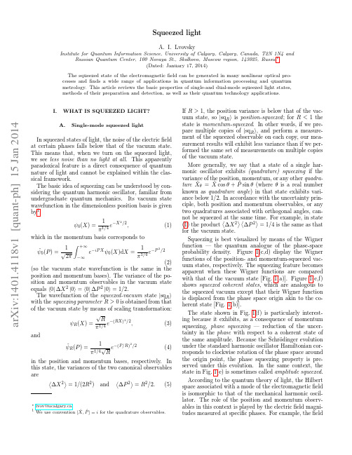
Squeezed lightA. I. LvovskyInstitute for Quantum Information Science, University of Calgary, Calgary, Canada, T2N 1N4 and Russian Quantum Center, 100 Novaya St., Skolkovo, Moscow region, 143025, Russia∗ (Dated: January 17, 2014) The squeezed state of the electromagnetic field can be generated in many nonlinear optical processes and finds a wide range of applications in quantum information processing and quantum metrology. This article reviews the basic properties of single-and dual-mode squeezed light states, methods of their preparation and detection, as well as their quantum technology applications.I.WHAT IS SQUEEZED LIGHT? A. Single-mode squeezed lightIn squeezed states of light, the noise of the electric field at certain phases falls below that of the vacuum state. This means that, when we turn on the squeezed light, we see less noise than no light at all. This apparently paradoxical feature is a direct consequence of quantum nature of light and cannot be explained within the classical framework. The basic idea of squeezing can be understood by considering the quantum harmonic oscillator, familiar from undergraduate quantum mechanics. Its vacuum state wavefunction in the dimensionless position basis is given by1 1 −X 2 /2 e , π 1/4 which in the momentum basis corresponds to ψ0 (X ) = ˜0 (P ) = √1 ψ 2π+∞(1)e−iP X ψ0 (X )dX =−∞1 π 1 /4e −P2/2(2) (so the vacuum state wavefunction is the same in the position and momentum bases). The variance of the position and momentum observables in the vacuum state equals 0| ∆X 2 |0 = 0| ∆P 2 |0 = 1/2. The wavefunction of the squeezed-vacuum state |sqR with the squeezing parameter R > 0 is obtained from that of the vacuum state by means of scaling transformation: √ 2 R ψR (X ) = 1/4 e−(RX ) /2 , (3) π and 2 1 ˜R (P ) = √ e−(P/R) /2 ψ (4) 1 / 4 π R in the position and momentum bases, respectively. In this state, the variances of the two canonical observables are ∆X 2 = 1/(2R2 ) and ∆P 2 = R2 /2. (5)∗ 1lvov@ucalgary.ca ˆ P ˆ ] = i for the quadrature observables. We use convention [X,If R > 1, the position variance is below that of the vacuum state, so |sqR is position-squeezed ; for R < 1 the state is momentum-squeezed. In other words, if we prepare multiple copies of |sqR , and perform a measurement of the squeezed observable on each copy, our measurement results will exhibit less variance than if we performed the same set of measurements on multiple copies of the vacuum state. More generally, we say that a state of a single harmonic oscillator exhibits (quadrature) squeezing if the variance of the position, momentum, or any other quadraˆθ = X ˆ cos θ + P ˆ sin θ (where θ is a real number ture X known as quadrature angle ) in that state exhibits variance below 1/2. In accordance with the uncertainty principle, both position and momentum observables, or any two quadratures associated with orthogonal angles, cannot be squeezed at the same time. For example, in state (1) the product ∆X 2 ∆P 2 = 1/4 is the same as that for the vacuum state. Squeezing is best visualized by means of the Wigner function — the quantum analogue of the phase-space probability density. Figure 1(c,d) display the Wigner functions of the position- and momentum-squeezed vacuum states, respectively. The squeezing feature becomes apparent when these Wigner functions are compared with that of the vacuum state [Fig. 1(a)]. Figure 1(e,f) shows squeezed coherent states, which are analogous to the squeezed vacuum except that their Wigner function is displaced from the phase space origin akin to the coherent state [Fig. 1(b)]. The state shown in Fig. 1(f) is particularly interesting because it exhibits, as a consequence of momentum squeezing, phase squeezing — reduction of the uncertainty in the phase with respect to a coherent state of the same amplitude. Because the Schr¨ odinger evolution under the standard harmonic oscillator Hamiltonian corresponds to clockwise rotation of the phase space around the origin point, the phase squeezing property is preserved under this evolution. In the same context, the state in Fig. 1(e) is sometimes called amplitude squeezed. According to the quantum theory of light, the Hilbert space associated with a mode of the electromagnetic field is isomorphic to that of the mechanical harmonic oscillator. The role of the position and momentum observables in this context is played by the electric field magnitudes measured at specific phases. For example, the fieldarXiv:1401.4118v1 [quant-ph] 15 Jan 20142 at phase zero (with respect to a certain reference) corresponds to the position observable, that at phase π/2 to the momentum observable, and so on. Accordingly, phase-sensitive measurements of the field in an electromagnetic wave are affected by quantum uncertainties. For the coherent and vacuum states, this uncertainty is ω/2ε0 V (the standard phase-independent and equals quantum limit, or SQL), where ω is the optical frequency and V is the quantization volume [1]. But squeezed optical states exhibit uncertainties below SQL at certain phases. Dependent on whether the mean coherent amplitude of the state is zero, squeezed optical states are classified into squeezed vacuum and (bright) squeezed light. Squeezed coherent states form a subset of bright squeezed light states. zero while its variance equals ∆X 2 = ψ | (ˆ a+a ˆ † )2 1 |ψ = − s, 2 2 (7)so for state |ψ is position squeezed for positive s.a)pump crystalb)pump photon pair crystal photon pairFIG. 2. Spontaneous parametric down-conversion. a) Degenerate configuration, leading to single-mode squeezed vacuum. b) Non-degenerate configuration, leading to two-mode squeezed vacuum.a)2 -2 -2b)P-2 0 2 4 6X-2 0 2P2 -2 -2P-2 0 2 4 6X-2 0 2P246XDj 246Xc)2 -2 -2d)P-2 0 2 4 6X6-2 0 2P-22P-2 0 2 4 6X6-2 0 2P24X2 -24Xe)2 -2 -2f)P-2 0 2 4 6X6-2 0 2P-22P24X-2 0 2 4 6 -2 0 2 Dj X 2 4 6XP-2FIG. 1. Wigner functions of certain single-oscillator states. a) Vacuum state. b) coherent state. c,d) Position- and momentum-squeezed vacuum states. e,f) Position- and momentum-squeezed coherent states with real amplitudes. Panels (b) and (f) show the phase uncertainties of the respective states to emphasize the phase squeezing of state (f). Insets show wavefunctions in the position and momentum bases.This result illustrates one of the primary methods of producing squeezing. Spontaneous parametric downconversion (SPDC) is a nonlinear optical process in which a photon of a powerful laser field propagating through a second-order nonlinear optical medium may split into two photons of lower energy. The frequencies, wavevectors and polarizations of the generated photons are governed by phase-matching conditions. Single-mode squeezing, such as that in the above example, is obtained when SPDC is degenerate : the two generated photons are indistinguishable in all their parameters: frequency, direction, and polarization. The quantum state of the optical mode into which the photon pairs are emitted exhibits squeezing [Fig. 2(a)]. Aside from being an interesting physical entity by itself, squeezed light has a variety of applications. One of the primary applications of single-mode squeezed light is in precision measurements of distances. Such measurements are typically done by means of interferometry. Quantum phase noise poses an ultimate limit to interferometry, and the application of squeezing (in particular, the phase squeezed state discussed above) permits expanding this limit beyond a fundamental boundary. For example, squeezing is employed in the new generation of gravitational wave detectors — GEO 600 in Europe and LIGO in the United States.B. Two-mode squeezed lightHow can one generate optical squeezed states in experiment? Consider the state s |ψ = |0 − √ |2 , 2 (6)where |0 and |2 are photon number (Fock) states and s is a real positive number. We assume s to be small, so the norm of state (6) is close to one. √ The mean value of ˆ = (ˆ the position operator X a+a ˆ† )/ 2 in this state isA state that is closely related to the single-oscillator squeezed vacuum in its theoretical description and experimental procedures, but quite different in properties is the two-mode squeezed vacuum (TMSV), also known as the twin-beam state. As the name suggests, this is a state of not one, but two mechanical or electromagnetic oscillators. We introduce this state by first analyzing the tensor product |0 ⊗ |0 of vacuum states of the two oscillators. In the position basis, its wavefunction [Fig. 3(a)],2 2 1 Ψ00 (Xa , Xb ) = √ e−Xa /2 e−Xb /2 π(8)3 can be rewritten as2 2 1 Ψ00 (Xa , Xb ) = √ e−(Xa −Xb ) /4 e−(Xa +Xb ) /4 . πboth Alice’s and Bob’s observables: (9) 1 −(Pa −Pb )2 /(4R2 ) −R2 (Pa +Pb )2 /4 ˜ R (Pa , Pb ) = √ Ψ e e . (11) π We see that for R > 1 Alice’s and Bob’s momenta are √ anticorrelated, i.e. the variance of the sum (Pa + Pb )/ 2 is below the level expected from two vacuum states [Fig. 3(d)]. The two-mode squeezed vacuum does not imply squeezing in each individual mode. On the contrary, Alice’s and Bob’s position and momentum observables in TMSV obey a Gaussian probability distribution with variance2 2 2 2 ∆Xa = ∆Xb = ∆ Pa = ∆ Pb =Here, Xa and Xb are the position observables of the two oscillators which are traditionally associated with fictional experimentalists Alice and Bob. The meaning √ of Eq. (9) √ is that the observables (Xa − Xb )/ 2 and (Xa + Xb )/ 2 have a Gaussian distribution with variance 1/2. This is not surprising because in the double-vacuum state Alice’s and Bob’s position observables are uncorrelated and both of them have variance 1/2. The behavior of the momentum quadratures in this state is analogous to that of the position.a)4 2 -4 -2 -2 -4XB4 2 2 4PB1 + R4 . 4R2(12)XA-4-2 -2 -424PAthat exceeds that of the vacuum state for any R = 1. In other words, each mode of a TMSV considered individually is in the thermal state. With increasing R > 1, the uncertainty of individual quadratures increases while that of the difference of Alice’s and Bob’s position observables as well as the sum of their momentum observables decreases. In the extreme case of R → ∞, the wavefunctions of the two-modes squeezed state take the form ΨR (Xa , Xb ) ∝ δ (Xa − Xb ) ˜ R (Pa , Pb ) ∝ δ (Pa + Pb ) Ψ (13) (14)b)4 2 -4 -2 -2 -4XB4 2 2 4PBXA-4-2 -2 -424PAFIG. 3. Wavefunctions (not Wigner functions!) of two-mode states in the position (left) and momentum (right) bases. a) Double-vacuum state is uncorrelated in both bases. b) The two-mode squeezed state with position observables correlated, and momentum observables anticorrelated beyond the standard quantum limit.The wavefunction of the two-mode squeezed vacuum state |TMSVR is given by2 2 2 2 1 ΨR (Xa , Xb ) = √ e−(Xa +Xb ) /(4R ) e−R (Xa −Xb ) /4 , π (10) where R, as previously, is the squeezing parameter [Fig. 3(c)]. In contrast to the double-vacuum, TMSV is an entangled state, and Alice’s and Bob’s position observables are nonclassically correlated thanks to that √ entanglement. For R > 1, the variance of (Xa − Xb )/ 2 is less than 1/2, i.e. below the value for the double vacuum state. The wavefunction of TMSV in the momentum basis is obtained from Eq. (10) by means of Fourier transform byBoth Alice’s and Bob’s positions are completely uncertain, but at the same time precisely equal, whereas the momenta are precisely opposite. This state is the basis of the famous quantum nonlocality paradox in its original formulation of Einstein, Podolsky and Rosen (EPR) [2]. EPR argued that by choosing to perform either a position or momentum measurement on her portion of the TMSV, Alice remotely prepares either a state with a certain position or one with a certain momentum at Bob’s location. But according to the uncertainty principle, certainty of position implies complete uncertainty of momentum, and vice versa. In other words, by choosing the setting of her measurement apparatus, Alice can instantly and remotely, without any interaction, prepare at Bob’s station one of two mutually incompatible physical realities. This apparent contradiction to basic principles of causality has lead EPR to challenge quantum mechanics as complete description of physical reality and triggered a debate that continues to this day. Experimental realization of TMSV is largely similar to that of single-mode squeezing. SPDC is the primary method; however, in contrast to the single-mode case, it is implemented in the non-degenerate configuration. The photons is each generated pair are emitted into two distinguishable modes that become carriers of the TMSV state [Fig. 2(b)]. In order to understand how non-degenerate SPDC leads to squeezing, consider the two-mode state |Ψ = |0 ⊗ |0 + s |1 ⊗ |1 , (15)4 i.e. a pair of photons has been emitted into Alice’s and Bob’s modes with amplitude s. Now √ if we evaluate the variance of the observable (Xa − Xb )/ 2, we find 1 1 1 ∆(Xa − Xb )2 = Ψ| (ˆ a+a ˆ† − ˆ b−ˆ b† )2 |Ψ = − s, 2 4 2 (16) i.e. Alice’s and Bob’s position observables are correlated akin to TMSV. A similar calculation shows anticorrelation of Alice’s and Bob’s momentum observables. Both the single-mode and two-mode squeezed vacuum states are valuable resources in quantum optical information technology. TMSV, in particular, is useful for generating heralded single photons and unconditional quantum teleportation.II. SALIENT FEATURES OF SQUEEZED STATES A. The squeezing operatorIf this evolution continues for time t, we will have ˆ (t) = S ˆ † (r )X ˆ (0)S ˆ (r ) = X ˆ (0)e−r ; X ˆ (t) = S ˆ † (r )P ˆ (0)S ˆ(r) = P ˆ (0)er , P (24a) (24b)which corresponds to position squeezing by factor R = er and corresponding momentum antisqueezing (Fig. 4). If the initial state is vacuum, the evolution will result in a squeezed vacuum state; coherent states will yield squeezed light [3]. As a self-check, we find the factor of quadrature squeezing in state (18), in analogy to Eq. (7): R= 0|∆X 2 |0 = ˆ† (r)∆X 2 S ˆ(r)|0 0|S 1/2 ≈1+r 1/2 − rwhich is in agreement with R = er for small r. The corresponding transformation of the creation and annihilation operators is given by a ˆ(t) = a ˆ(0) cosh r − a ˆ† (0) sinh r; a ˆ† (t) = a ˆ† (0) cosh r − a ˆ(0) sinh r, known as Bogoliubov transformation. (25a) (25b)We now proceed to a more rigorous mathematical description of squeezing. Single-mode squeezing occurs under the action of operator ˆ(ζ ) = exp[(ζ a S ˆ2 − ζ ∗ a ˆ†2 )/2], (17)Pwhere ζ = reiφ is the squeezing parameter, with r and φ being real numbers, upon the vacuum state. Phase φ determines the angle of the quadrature that is being squeezed. In the following, we assume this phase to be zero so ζ = r. Note that, for a small r, the squeezing operator (17) acting on the vacuum state, generates state √ ˆ(r) |0 ≈ [1+(ra S ˆ2 −r a ˆ†2 )/2] |0 = |0 −(r/ 2) |2 , (18) which is consistent with Eq. (6) for s = r. The action of the squeezing operator can be analyzed as fictitious evolution under Hamiltonian ˆ = i α[ˆ H a2 − (ˆ a† )2 ]/2 (19)Xˆ )t ˆ(r) = e−i(H/ for time t = r/α (so that S ). Analyzing this evolution in the Heisenberg picture, we use [ˆ a, a ˆ† ] = 1 to find that˙ = i [H, ˆ a a ˆ ˆ] = −αa ˆ† and ˙ † = −αa a ˆ ˆ.(20)FIG. 4. Transformation of quadratures under the action of the squeezing Hamiltonian (19) with α > 0. Grey areas show examples of Wigner function transformations with r = αt = ln 2.(21)Now using the expressions for quadrature observables √ √ ˆ = (ˆ ˆ = (ˆ X a+a ˆ† )/ 2 and P a−a ˆ† )/ 2i, (22) we rewrite Eqs. (20) and (21) as ˙ ˆ X = −αX ; ˙ ˆ P = αP. (23a) (23b)Two-mode squeezing is treated similarly. The twomode squeezing operator is ˆ2 (ζ ) = exp[(−ζ a S ˆˆ b + ζ ∗a ˆ†ˆ b† )]. (26)Assuming, again, a real ζ = r, introducing the fictitious Hamiltonian and recalling that the creation and annihilation operators associated with different modes commute,5 we find a ˆ(t) = a ˆ(0) cosh r + ˆ b(0)† sinh r; ˆ b(t) = ˆ b(0) cosh r + a ˆ(0)† sinh r; and hence ˆ a (t) ± X ˆ b (t) = [X ˆ a (0) ± X ˆ b (0)]e±r ; X ˆa (t) ± P ˆb (t) = [P ˆa (0) ± P ˆb (0)]e∓r . P (28a) (28b) (27a) (27b) Decomposing the exponent in right-hand side of the above equation into the Taylor series with respect to α, we obtain α 2m . m! n=0 m=0 (33) Because this equality must hold for any real α, each term of the sum in the left-hand side must equal its counterpart in the right-hand side that contains the same power of α. Hence n = 2m and 2R 1 + R2 2m |sqR = 1 − R2 2R 1 + R2 2(1 + R2 )m ∞αn n |sqR √ = n!∞1 − R2 2(1 + R2 )mInitially, Alice’s and Bob’s modes are in vacuum states, and the quadrature observables in these modes are uncorrelated. But as the time progresses, Alice’s and Bob’s position observables become correlated while the momentum observables become anticorrelated.(2m)! . m!(34)Since R = er , we haveB. Photon number statistics1 2R = 1 + R2 cosh rand1 − R2 = − tanh r, 1 + R2(35)An important component in the theoretical description of squeezed light is its decomposition in the photon number basis, i.e. calculating the quantities n |sqR for the single-mode squeezed state and mn |TMSVR for the two-mode state. Due to non-commutativity of the photon creation and annihilation operators, this calculation turns out surprisingly difficult even for basic squeezed vacuum states, let alone squeezed coherent states and the states that have been affected by losses. Possible approaches to this calculation include the disentangling theorem for SU(1,1) Lie algebra [4], direct calculation of the wavefunction overlap in the position space [5] or transformation of the squeezing operator [6]. Here we derive the photon number statistics of single- and twomode squeezed vacuum states by calculating their inner product with coherent states. The wavefunction of a coherent state with real amplitude α is ψα (X ) = 1 π 1/4 e−(X −α√ 2)2 /2so Eq. (34) can be rewritten as |sqR = √ 1 cosh r∞(− tanh r)mm=0(2m)! |2m . 2m m!(36)We stop here for a brief discussion. First, we note that that for r 1, Eq. (36) becomes √ |sqR = |0 − (r/ 2) |2 + O(r2 ), (37),(29)so its inner product with the position squeezed state (3) equalsR2 2R − 1+ α2 R2 . e 2 1+R −∞ (30) Now we recall that the coherent state is decomposed into the Fock basis according to+∞α |sqR =ψα (X )ψR (X )dX =∞|α =n=0e −α2/2αn √ |n , n!(31)consistently with Eq. (18). Second, note that the squeezed vacuum state (36) contains only terms with even photon numbers. This is a fundamental feature of this state; in fact, one of the earlier names for squeezed states has been “two-photon coherent states” [7]. This feature follows from the nature of the squeezing operator (17): in its decomposition into the Taylor series with respect to r, creation and annihilation operators occur only in pairs. Pairwise emission of photons is also a part of the physical nature of SPDC: due to energy conservation a pump photon can only split into two photons of half its energy. We now turn to finding the photon number decomposition of the two-mode squeezed state. We first notice, by looking at Eq. (26), that |RAB must only contain terms with equal photon numbers in Alice’s and Bob’s modes. This circumstance allows us to significantly simplify the algebra. We proceed along the same route as outlined above, calculating the overlap of |RAB with the tensor product |αα of identical coherent states |α in Alice’s and Bob’s channels using Eqs. (10) and (29): αα|TMSVR+∞so we have∞= α n |sqR √ = n!nψα (Xa )ψα (Xb )ΨR (Xa , Xb )dXa dXb−∞n=02R e 1 + R21−R2 α2 2(1+R2 )(32)=2R − 1+2R2 α2 e . 1 + R2(38)6 Decomposing the coherent states in the left-hand side into the Fock basis according to Eq. (31) and keeping only the terms with equal photon numbers, we have∞−R2 2 2R − 1 α2n α e 1+R2 nn| TMSVR √ = 2 1+R n!(39)n=0Now writing the Taylor series for the right-rand side and using Eq. (35), we obtain |TMSVR = 1 tanhn r |nn . cosh r n=0∞(40)FIG. 5. Experimentally reconstructed photon number statistics of the squeezed vacuum state. For low photon numbers, the even terms are greater than the odd terms due to pairwise production of photons, albeit the odd term contribution is nonzero due to loss. Reproduced from Ref. [10].position-squeezed vacuum ˆ¢(t ) bˆ¢(t ) a momentum-squeezed vacuumSimilarly to the single-mode squeezing, it is easy to verify that result is consistent with state (15) for small r. On the other hand, in contrast to the single-mode case, the energy spectrum of TMSV follows Boltzmann distribution with mean photon number in each mode n = sinh2 r. This is in agreement with our earlier observation that Alice’s and Bob’s portions of TMSV considered independently of their counterpart are in the thermal state, i.e. the state whose photon number distribution obeys Boltzmann statistics with the temperature given by e− ω/kT = tanh r. While the present analysis is limited to pure squeezed vacuum states, photon number decompositions of squeezed coherent states and squeezed states that have undergone losses can be found in the literature [8, 9]. In contrast to pure squeezed vacuum states, these decompositions have nonzero terms associated to non-paired photons. The origin of these terms is easily understood. If a one- or two-mode squeezed vacuum state experiences a loss, it may happen that one of the photons in a pair is lost while the other one remains. If the squeezing operator acts on a coherent state, the odd photon number terms will appear in the resulting state because they are present initially. Photon statistics of both classes of squeezed states have been tested experimentally, as discussed in Section III below. An example is shown in Fig. 5.ˆ0 a fictitious input vacuum ˆ0 bˆ(0) b input vacuum2-mode squeezerˆ(0) aˆ(t ) a two-mode squeezed vacuum ˆ(t ) bFIG. 6. Interconversion of the two-mode squeezed vacuum and two single-mode squeezed vacuum states. Dashed lines show a fictitious beam splitter transformation of a pair of vacuum states such that the modes a ˆ (t), ˆ b (t) are explicitly single-mode squeezed with respect to modes a ˆ 0, ˆ b 0.In accordance with the definition (22) of quadrature observables, Eqs. (41) apply in the same way to the position and momentum of the input and output modes. Applying this to Eqs. (28), we find √ ˆ a,b = [X ˆ a (t) ∓ X ˆ b (t)]/ 2 X √ ˆ a (0) ∓ X ˆ b (0)]/ 2 = e ∓r [ X (42) for the output positions and √ ˆa,b = [P ˆa (t) ∓ P ˆb (t)]/ 2 P √ ˆa (0) ∓ P ˆb (0)]/ 2 = e ±r [ PC.Interconversion between single- and two-mode squeezing(43)If the modes of the TMSV are overlapped on a symmetric beam splitter, two unentangled single-mode vacuum states will emerge in the output (Fig. 6). To see this, we recall the beam splitter transformation a ˆ = τa ˆ − ρˆ b; ˆ ˆ b = τ b + ρa ˆ, (41a) (41b)for the momenta. In order to understand what state this corresponds to, let us assume, for the sake of the argument, that vacuum modes a ˆ and ˆ b at the SPDC input have been obtained from another pair of modes by means of another symmetric beam splitter: √ a ˆ0 = [ˆ a(0) − ˆ b(0)]/ 2 (44) √ 0 ˆ ˆ b = [ˆ a(0) + b(0)]/ 2. (45) Of course, since modes a ˆ(0) and ˆ b(0) are in the vacuum 0 0 ˆ state, so are a ˆ and b . We then have:0 ˆ a,b = e∓r X ˆ a,b X ; ±r ˆ 0 ˆ Pa,b = e Pa,b ,where τ and ρ are the beam splitter amplitude transmissivity and reflectivity, respectively. For a symmetric √ beam splitter, τ = ρ = 1/ 2. In writing Eqs. (41), we neglected possible phase shifts that may be applied to individual input and output modes [5].(46)7 where superscript 0 associates the quadrature with modes a ˆ0 and ˆ b0 . We see that modes a ˆ and ˆ b are re0 0 ˆ lated to vacuum modes a ˆ and b by means of position and momentum squeezing transformations, respectively. Because the beam-splitter transformation is reversible, it can also be used to obtain a TMSV from two singlemode squeezed vacuum states with squeezing in orthogonal quadratures. This technique has been used, for example, in the experiment on continuous-variable quantum teleportation [11].E. Effect of lossesD.Squeezed vacuum and squeezed lightSqueezed vacuum and bright squeezed light are readily converted between each other by means of the phasespace displacement operator [5], whose action in the Heisenberg picture can be written as ˆ † (α)ˆ ˆ (α) = a D a† D ˆ + α. (47)Squeezed states that occur in practical experiments necessarily suffer from losses present in sources, transmission channels and detectors. In order to understand the effect of propagation losses on a single-mode squeezed vacuum state, we can use the model in which a lossy optical element with transmission T is replaced by a beam splitter (Fig. 8). At the other input port of the beam splitter there is a vacuum state. The interference of the signal mode a ˆ with the vacuum mode v ˆ will produce a mode with operator a ˆ = τa ˆ − ρv ˆ (with τ 2 = T and ρ2 = 1 − T being the beam splitter transmissivity and reflectivity) in the beam splitter output. Accordingly, we have ˆ θ,out = τ X ˆ a,θ − ρX ˆ v,θ . X (52)This means, in particular, that the position and momentum transform according to √ ˆ →X ˆ + Re α 2; (48) X √ ˆ ˆ P → P + Im α 2, (49) ˆ (α), the entire phase space disso, under the action of D places itself, thereby changing the coherent amplitude of the squeezed state without changing the degree of squeezing.Because the quadrature observable of the signal and vacuum states are uncorrelated, and since ∆(Xθ )2 = 1/2, it follows that2 2 ∆Xθ, ∆(Xa,θ )2 + ρ2 ∆(Xv,θ )2 out = τ= T ∆(Xa,θ )2 + (1 − T )/2.(53)Analyzing Eqs. (41) we see that the optical loss alone, no matter how significant, cannot eliminate the property of squeezing completely.ˆ alow-reflectivity beam splitterˆ - rb aˆ aˆ b b1signalˆout aoutputFIG. 7. Implementation of phase-space displacement. ρ is the beam splitter’s amplitude reflectivity.ˆ vacuum vFIG. 8. The beam splitter model of loss.Phase-space displacement can be implemented experimentally by overlapping the signal state with a strong coherent state |β on a low-reflectivity beam splitter (Fig. 7). Applying the beam splitter transformation (41), we find for the signal mode a ˆ = τa ˆ − ρˆ b (50)Given that mode ˆ b is in a coherent state (i.e. an eignestate of ˆ b) and that ρ 1 (i.e. τ ∼ 1), we have a ˆ =a ˆ − ρβ (51)in analogy to Eq. (47). The displacement operation has been used to change the amplitude of squeezed light in many experiments, for example, in Ref. [12].Ideal squeezed-vacuum and coherent states have the minimum-uncertainty property: the product of uncer2 2 tainties ∆Xout ∆Pout reaches the theoretical minimum of 1/4. But this is no longer the case in the presence of losses. The deviation of the uncertainty from the minimum can be used to estimate the preparation quality of a squeezed state. Suppose a measurement of a squeezed state yielded the minimum and maximum quadrature un2 2 and ∆Xmax , respectively. certainty values of ∆Xmin One can assume that the state has been obtained from an ideal (minimum-uncertainty) squeezed state with squeezing R by means of loss channel with transmissivity T . Using Eq. (5) and solving Eqs. (53), one finds T [13], which can then be compared with the values expected from the setup at hand.。

a rXiv:h ep-ph/9911527v13Nov1999ADP-99-49/T3851/m Q Corrections to the Bethe-Salpeter Equation for ΛQ in the Diquark Picture X.-H.Guo 1,2,A.W.Thomas 1and A.G.Williams 1,31Department of Physics and Mathematical Physics,and Special Research Center for the Subatomic Structure of Matter,University of Adelaide,SA 5005,Australia 2Institute of High Energy Physics,Academia Sinica,Beijing 100039,China 3Department of Physics and SCRI,Florida State University,Tallahassee,FL 32306-4052e-mail:xhguo@.au,athomas@.au,awilliam@.au Abstract Corrections of order 1/m Q (Q =b or c )to the Bethe-Salpeter (B-S)equa-tion for ΛQ are analyzed on the assumption that the heavy baryon ΛQ is composed of a heavy quark and a scalar,light diquark.It is found that in addition to the one B-S scalar function in the limit m Q →∞,two morescalar functions are needed at the order 1/m Q .These can be related tothe B-S scalar function in the leading order.The six form factors for theweak transition Λb →Λc are expressed in terms of these wave functions andthe results are consistent with HQET to order 1/m Q .Assuming the kernelfor the B-S equation in the limit m Q →∞to consist of a scalar confine-ment term and a one-gluon-exchange term we obtain numerical solutions forthe B-S wave functions,and hence for the Λb →Λc form factors to order1/m Q .Predictions are given for the differential and total decay widths forΛb →Λc l ¯ν,and also for the nonleptonic decay widths for Λb →Λc plus apseudoscalar or vector meson,with QCD corrections being also included.PACS Numbers :11.10.St,12.39.Hg,14.20.Mr,14.20.LqI.IntroductionHeavyflavor physics provides an important area within which to study many important physical phenomena in particle physics,such as the structure and interac-tions inside heavy hadrons,the heavy hadron decay mechanism,and the plausibility of present nonperturbative QCD models.Heavy baryons have been studied much less than heavy mesons,both experimentally and theoretically.However,more ex-perimental data for heavy baryons is being accumulated[1,2,3,4,5,6]and we expect that the experimental situation for them will continue to improve in the near future.On the theoretical side,heavy quark effective theory(HQET)[7]provides a systematic way to study physical processes involving heavy hadrons.With the aid of HQET heavy hadron physics is simplified when m Q≫ΛQCD.In order to get the complete physics,HQET is usually combined with some nonperturbative QCD models which deal with dynamics inside heavy hadrons.As a formally exact equation to describe the hadronic bound state,the B-S equation is an effective method to deal with nonperturbative QCD effects.In fact, in combination with HQET,the B-S equation has already been applied to the heavy meson system[8,9,10].The Isgur-Wise function was calculated[8,10]and1/m Q corrections were also considered[8].In previous work[11,12,13],we established the B-S equations in the heavy quark limit(m Q→∞)for the heavy baryons ΛQ andω(∗)Q(whereω=Ξ,ΣorΩand Q=b or c).These were assumed to be composed of a heavy quark,Q,and a light scalar and axial-vector diquark, respectively.We found that in the limit m Q→∞,the B-S equations for these heavy baryons are greatly simplified.For example,only one B-S scalar function is needed forΛQ in this limit.By assuming that the B-S equation’s kernel consists of a scalar confinement term and a one-gluon-exchange term we gave numerical solutions for the B-S wave functions in the covariant instantaneous approximation, and consequently applied these solutions to calculate the Isgur-Wise functions forthe weak transitionsΛb→Λc andΩ(∗)b→Ω(∗)c.In reality,the heavy quark mass is not infinite.Therefore,in order to give moreexact phenomenological predictions we have to include1/m Q corrections,especially1/m c corrections.It is the purpose of the present paper to analyze the1/m Q cor-rections to the B-S equation forΛQ and to give some phenomenological predictionsfor its weak decays.As in the previous work[11,12,13,14],we will still assumethatΛQ is composed of a heavy quark and a light,scalar diquark.In this picture,the three body system is simplified to a two body system.In the framework of HQET,the eigenstate of HQET Lagrangian|ΛQ HQET has 0+light degrees of freedom.This leads to only one Isgur-Wise functionξ(ω)(ωis the velocity transfer)forΛb→Λc in the leading order of the1/m Q expansion [15,16,17,18,19,20].When1/m Q corrections are included,another form factor inHQET and an unknownflavor-independent parameter which is defined as the massdifference mΛQ−m Q in the heavy quark limit are involved[19].This provides some relations among the six form factors forΛb→Λc to order1/m Q.Consequently,if one form factor is determined,the otherfive form factors can be obtained.Here we extend our previous work to solve the B-S equation forΛQ to order1/m Q,in combination with the results of HQET.It can be shown that two B-S scalar functions are needed at the order1/m Q,in addition to the one scalarfunction in the limit m Q→∞.The relationship among these three scalar functions can be found.Therefore,our numerical results for the B-S wave function in the order m Q→∞can be applied directly to obtain the1/m Q corrections to the form factors for the weak transitionΛb→Λc.It can be shown that the relations among all the six form factors forΛb→Λc in the B-S approach are consistent with those from HQET to order1/m Q.We also give phenomenological predictions for the differential and total decay widths forΛb→Λc l¯ν,and for the nonleptonic decay widths forΛb→Λc plus a pseudoscalar or vector meson.Since the QCD correctionsare comparable with the1/m Q corrections,we also include QCD corrections in our predictions.Furthermore,we discuss the dependence of our results on the various input parameters in our model,and present the comparison of our results with those of other models.The remainder of this paper is organized as follows.In Section II we discuss the B-S equation for the heavy quark and light scalar diquark system to order1/m Q and introduce the two B-S scalar functions appearing at this order.We also discuss the constraint on the form of the kernel.In Section III we express the six form factors forΛb→Λc in terms of the B-S wave function.The consistency of our model with HQET is discussed.We also present numerical solutions for these form factors.In Section VI we apply the solutions for theΛb→Λc form factors,with QCD corrections being included,to the semileptonic decayΛb→Λc l¯ν,and the nonleptonic decaysΛb→Λc plus a pseudoscalar or vector meson.Finally,Section VI contains a summary and discussion.II.The B-S equation forΛQ to1/m QBased on the picture thatΛQ is a bound state of a heavy quark and a light, scalar diquark,its B-S wave function is defined as[11]χ(x1,x2,P)= 0|TψQ(x1)ϕ(x2)|ΛQ(P) ,(1)whereψQ(x1)andϕ(x2)are thefield operators for the heavy quark Q and thev is the total momentum ofΛQ and light,scalar diquark,respectively,P=mΛQv is its velocity.Let m Q and m D be the masses of the heavy quark and the light diquark inΛQ,p be the relative momentum of the two constituents,and define.The B-S wave function in momentum space is defined λ1=m Qm Q+m Dasχ(x1,x2,P)=e iP X d4pwhere X=λ1x1+λ2x2is the coordinate of the center of mass and x=x1−x2. The momentum of the heavy quark is p1=λ1P+p and that of the diquark is p2=−λ2P+p.χP(p)satisfies the following B-S equation[21]χP(p)=S F(λ1P+p) d4qE1+O(1/m2Q),(5)m Qwhere E0and E1/m Q are binding energies at the leading andfirst order in the1/m Q expansion,respectively.m D,E0and E1are independent of m Q.Since we are considering1/m Q corrections to the B-S equation,we expand the heavy quark propagator S F(λ1P+p)to order1/m Q.Wefind1S F=S0F+,(7)2(p l+E0+m D+iǫ)andS1F=i (−E1+p2t/2)(1+/v)2(p l+E0+m D+iǫ)−1−/vIt can be shown that the light diquark propagator to1/m Q still keeps its form in the limit m Q→∞,S D=ip2t+m2D.Similarly to Eq.(6),we writeχP(p)and K(P,p,q)in the following form(to order 1/m Q):χP(p)=χ0P(p)+1m QK1(P,p,q),(10)whereχ1P(p)and K1(P,p,q)arise from1/m Q corrections.As in our previous work, we assume the kernel contains a scalar confinement term and a one-gluon-exchange term.Hence we have−iK0=I⊗IV1+vµ⊗(p2+p′2)µV2,−iK1=I⊗IV3+γµ⊗(p2+p′2)µV4,(11) where vµin K0appears because of the heavy quark symmetry.Substituting Eqs.(6)and(10)into the B-S equation(3)we have the integral equations forχ0P(p)andχ1P(p)χ0P(p)=S0F(λ1P+p) d4q(2π)4K1(P,p,q)χ0P(q)S D(−λ2P+p)+S1F(λ1P+p) d4q(2π)4K0(P,p,q)χ1P(q)S D(−λ2P+p).(13) Eq.(12)is what we obtained in the limit m Q→∞,which together with Eq.(7)gives/vχ0P(p)=χ0P(p),(14)since/v/v=v2=1and so/v S0F=S0F.Therefore,S0F(λ1P+p)γµχ0P(q)=S0F(λ1P+ p)vµχ0P(q)in thefirst term of Eq.(13).So to order1/m Q,the Dirac matrixγµfrom the one-gluon-exchange term in K1(P,p,q)can still be replaced by vµ.We divideχ1P(p)into two parts by definingχ1P(p)=χ+1P(p)+χ−1P(p),/vχ±1P(p)=±χ±1P(p),(15)i.e.,χ+1P(p)≡12[χ1P(p)−/vχ1P(p)].After writingdown all the possible terms forχ0P(p)andχ±1P(p),and considering the constraintson them,Eqs.(14)and(15),we obtain thatχ0P(p)=φ0P(p)uΛQ(v,s),χ+1P(p)=φ1P(p)uΛQ(v,s),χ−1P(p)=φ2P(p)/p t uΛQ(v,s),(16) whereφ0P(p),φ1P(p)andφ2P(p)are Lorentz scalar functions.Substituting Eq.(16)into Eqs.(12)(13)and using Eqs.(7)(8)(9)we haveφ0P(p)=−1(2π)4K0(P,p,q)φ0P(q),(17)φ1P(p)=−1(2π)4K0(P,p,q)φ1P(q)−1(2π)4[K1(P,p,q)+p2t/2−E12φ0P(p).(19)φ0P(p)is the B-S scalar function in the leading order of the1/m Q expansion, which was calculated in[11].From Eq.(19)φ2P(p)can be given in terms ofφ0P(p).The numerical solutions forφ0P(p)andφ1P(p)can be obtained by discretizing the integration region into n pieces(with n sufficiently large).In this way,the integral equations become matrix equations and the B-S scalar functionsφ0P(p)andφ1P(p) become n dimensional vectors.Thusφ0P(p)is the solution of the eigenvalue equation (A−I)φ0=0,where A is an n×n matrix corresponding to the right hand side of Eq.(17).In order to have a unique solution for the ground state,the rank of(A−I) should be n−1.From Eq.(18),φ1P(p)is the solution of(A−I)φ1=B,where B is an n dimensional vector corresponding to the second integral term on the right hand side of Eq.(18).In order to have solutions forφ1P(p),the rank of the augmented matrix(A−I,B)should be equal to that of(A−I),i.e.,B can be expressed as linear combination of the n−1linearly independent columns in(A−I).This is difficult to guarantee if B=0,since the way to divide(A−I)into n columns is arbitrary.Therefore,we demand the following condition in order to have solutions forφ1P(p)d4q p l+E0+m D+iǫK0(P,p,q) φ0P(q)=0.(20) Eq.(20)provides a constraint on the form of the kernel K1(P,p,q),in which E1is also related K1(P,p,q).In this way,φ1P(p)satisfies the same eigenvalue equation asφ0P(p).Therefore,we haveφ1P(p)=σφ0P(p),(21)whereσis a constant of proportionality,with mass dimension,which can be deter-mined by Luke’s theorem[22]at the zero-recoil point in HQET.We will discuss it in the next section.Since bothφ1P(p)andφ2P(p)can be related toφ0P(p),we can calculate the 1/m Q corrections without explicitly solving the integral equations forφ1P(p)and φ2P(p).In the previous work[11]φ0P(p)was solved by assuming that V1and V2inEq.(11)arise from linear confinement and one-gluon-exchange terms,respectively. In the covariant instantaneous approximation,˜V i≡V i|p l=q l,i=1,2,wefind˜V 1=8πκ(2π)38πκ3α(eff)2sQ20Q2+Q2,to describe the internal structure of the light diquark[23]. Defining˜φ0P(p t)= d p l2(E0−W p+m D)W pd3q t(p l+E0+m D+iǫ)(p2l−W2p+iǫ)d3q t−(G 1(ω)γµ+G 2(ω)v µ+G 3(ω)v ′µ)γ5]u Λb (v ),(25)where J µis the V −A weak current,v and v ′are the velocities of Λb and Λc ,respectively,and ω=v ′·v .The form factors F i and G i (i =1,2,3)are related to each other by the following equations,to order 1/m Q ,when HQET is applied [19]F1=G 1 1+ 1m b¯Λm c¯Λm b ¯Λ(2π)4¯χP ′(p ′)γµ(1−γ5)χP (p )S −1D (p 2),(27)where P (P ′)is the momentum of Λb (Λc ).¯χP ′(p ′)is the wave function of the final state Λc (v ′)which can also be expressed in terms of the three B-S scalar functions φ0P (p ),φ1P (p )and φ2P (p )in Eq.(16)¯χP (p )=¯u ΛQ (v,s ) φ0P (p )+1m c +11+ω =−i d 4km c[φ1P ′(k ′)−(k ′l +m D )φ2P ′(k ′)]φ0P (k )(k 2l −W 2k )+1m b(f1−f2)+1(2π)4 φ0P′(k′)φ0P(k)(k2l−W2k)+1m c[φ1P′(k′)−(k′l+m D)φ2P′(k′)]φ0P(k)(k2l−W2k)+1m bφ0P′(k′)[φ1P(k)−(k l+m D)φ2P(k)](k2l−W2k) +O(1/m2Q),(30) 11+ω+2(f1−m D F) =O(1/m2Q),(31)11+ω+2f2 =O(1/m2Q),(32) where we have defined f1,f2and F by the following equations,on the grounds of Lorentz invariance:d4k(2π)4φ2P′(k′)φ0P(k)kµ(k2l−W2k)=f1vµ+f2v′µ.(34) Eq.(34)leads tof1+f2=1(2π)4φ2P′(k′)φ0P(k)(k2l−W2k)(v·k+v′·k).(35)Eqs.(29)and(30)give the expression for G1to order1/m Q.From Eqs.(31)and (32)we can see that Eq.(29)is the same as Eq.(30).Therefore,we can calculate G1to1/m Q from either of these two equations.This indicates that our model is consistent with HQET to order1/m Q.Substituting Eq.(35)into Eq.(30)and using Eq.(19)we haveG1=−i d4k+12(k′l+m D)φ0P′(k′)]φ0P(k)(k2l−W2k)+12(k l+m D)φ0P(k)](k2l−W2k)+ 1m b 1ω2−1cosθ,k′2t=k2t+k2t(ω2−1)cos2θ+k2l(ω2−1)−2k l k tω√contour we haveG 1(ω)=ξ(ω)+1m bA b (ω),(41)whereξ(ω)=−d 3k t(2π)3(ω2−1)W k +ωk t√2(ω+1)F (ω,k t ),(43)A b (ω)=d 3k tω2−1cos θE 0+m D −ωW k −k t√(2π)3˜φ0P ′(r t )[˜V 1(k ′t −r t )−2(ωW k +k t√(2π)3ρ(q 2t )4π22ρ(q 2t )(2π)3ρ(q 2t )4π2ρ(q 2t )(|p t |−|q t |)2+δ2,(47)where ρ(q 2t )is some arbitrary function of q 2t .In our model we have several parameters,α(eff)s ,κ,Q 20,m D ,E 0and E 1.The parameter Q 20can be chosen as 3.2GeV 2from the data for the electromagnetic formfactor of the proton [23].As discussed in Ref.[11],we let κvary in the region between 0.02GeV 3and 0.1GeV 3.In HQET,the binding energies should satisfy the constraint Eq.(5).Note that m D +E 0and E 1are independent of the flavor of the heavy quark.From the B-S equation solutions in the meson case,it has been found that the values m b =5.02GeV and m c =1.58GeV give predictions which are in good agreementwith experiments[8].Since in the b-baryon case the O(1/m2b)corrections are very small,we use the following equation to discuss the relations among m D,E0and E1,m D+E0+1m bE1)/E0∼ΛQCDπv1,∆G1=ξαs(¯m)πv i,∆G i=−ξαs(¯m)where v i=v i(ω)and a i=a i(ω)(i=1,2,3)are the QCD corrections calculated from the next-to-leading order renormalization group improved perturbation theory. The scale¯m is chosen such that higher-order terms(αs ln(m b/m c))n(n>1)do not contribute.Consequently,it is not necessary to apply a renormalization group summation as far as only numerical evaluations are concerned.It is shown that¯m can be chosen as2m b m c/(m b+m c)≃2.3GeV.The detailed formulae for v i and a i can be found in[25],which also includes a discussion on the infra-red cutoffemployed in the calculation of the vertex corrections.As in[25],we choose this cutoffto be 200MeV which is afictitious gluon mass.Furthermore,we useΛQCD=200MeV in our numerical calculations.Fig.1The numerical results for F i(i=1,2,3)forκ=0.02GeV3(solid lines)andκ= 0.10GeV3(dotted lines),with m D=0.7GeV.From top to bottom we have F1,F3,and F2,respectively.A.Semileptonic decaysΛb→Λc l¯νMaking use of the general kinematical formulae by K¨o ner and Kr¨a mer[26],wefind for the differential decay width of Λb →Λc l ¯ν[14]dΓ3m 4Λc m Λb AF 21√m c+1πv 1(ω−1)[3(η+η−1)+2−4ω]+αsπ(ω2−1)[v 2(1+η)+v 3(1+η−1)+a 2(1−η)+a 3(η−1−1)],(50)where η=m Λc /m Λb and A =G 2F2+)+b (0−)through which Λc is detected,since the structure for such decays isalready well known.It should be noted that in Eq.(50)O (αs ¯Λ/m Q )corrections have been ignored and the lepton mass is set to zero.The plot for A −1dΓ204060801001201 1.05 1.1 1.15 1.2 1.25 1.3 1.35 1.4 1.45ωdΓFig.2The numerical results for A −1dΓTable1:Predictions for the decay rates forΛb→Λc l¯ν,in units1010s−1B(Λc→ab)m D(GeV)Γ0Γ1/mQ Γ1/mQ+QCD0.70 5.12(7.12) 4.60(6.56) 3.34(4.72)√1We note that the results without either1/m Q and QCD corrections in Table1are bigger than those presented in Ref.[11]by about18%.This is because we employed a cutoffin the numerical integrations in Ref.[11],while the integrations are carried out to infinity in the present work.that one of the currents in the Hamiltonian(51)is factorized out and generates a meson[27,28].Thus the decay amplitude of the two body nonleptonic decay be-comes the product of two matrix elements,one is related to the decay constant of the factorized meson(P or V)and the other is the weak transition matrix element betweenΛb andΛc,M fac(Λb→Λc P(V))=G F2V cb V∗UD a1 P(V)|Aµ(Vµ)|0 Λc(P′)|Jµ|Λb(P) ,(52) where 0|Aµ(Vµ)|P(V) are related to the decay constants of the pseudoscalar meson or vector meson by0|Aµ|P =if P qµ,0|Vµ|V =f V m Vǫµ,(53) where qµis the momentum of the meson emitted from the W-boson andǫµis the polarization vector of the emitted vector meson.It is noted that in the two-body nonleptonic weak decaysΛb→Λc P(V)there is no contribution from the a2term since such a term corresponds to the transition ofΛb to a light baryon instead ofΛc. On the other hand,the general form for the amplitudes ofΛb→Λc P(V)are M(Λb→Λc P)=i¯uΛc(P′)(A+Bγ5)uΛb(P),M(Λb→Λc V)=¯uΛc(P′)ǫ∗µ(A1γµγ5+A2P′µγ5+B1γµ+B2P′µ)uΛb(P).(54)Alternatively,the matrix element forΛb→Λc can be expressed as the following on the ground of Lorentz invarianceΛc(P′)|Jµ|Λb(P) =¯uΛc(P′)[f1(q2)γµ+if2(q2)σµνqν+f3(q2)qµ−(g1(q2)γµ+ig2(q2)σµνqν+g3(q2)qµ)γ5]uΛb(P),(55) where f i,g i(i=1,2,3)are the Lorentz scalars.The relations between f i,g i andF i,G i aref1=F1+1mΛb+F32 F2mΛc ,f3=1mΛb−F32(mΛb−mΛc)G2mΛc,g2=1mΛb+G32 G2mΛc.(56)The decay widths and the up-down asymmetries forΛb→Λc P(V)are available in Refs.[29][30]:Γ(Λb→Λc P)=| P′|m2Λb|A|2+(mΛb−mΛc)2−m2P(EΛc+mΛc)|A|2+(EΛc−mΛc)|B|2,(57)where A and B are related to the form factors byA=G F2V cb V∗UD a1f P[(mΛb−mΛc)f1(m2P)+m2P f3(m2P)],B=G F2V cb V∗UD a1f P[(mΛb+mΛc)g1(m2P)−m2P g3(m2P)],(58)andΓ(Λb→Λc V)=| P′|mΛb2(|S|2+|P2|2)+E2V2m2V(|S|2+|P2|2)+E2V(|S+D|2+|P1|2),(59) whereS=−A1,D=−|P′|2P1=−| P′|EΛc+mΛcB1+mΛbB2),P2=|P′|√√√√Table2:Predictions for the decay rates(in units1010s−1a21,which is defined in Eq.(51)),and the asymmetry parameters forΛb→Λc P(V)ProcessΓ0Γ1/mQ Γ1/mQ+QCDα1/mQ+QCDΛ0b→Λ+cρ−0.44(0.78)0.51(0.94)0.42(0.77)-0.89Λ0b→Λ+c D∗−s0.78(1.17)0.89(1.35)0.76(1.15)-0.38Λ0b→Λ+c K∗−0.023(0.041)0.027(0.049)0.022(0.040)-0.85Λ0b→Λ+c D∗−0.027(0.041)0.031(0.048)0.026(0.040)-0.42In our previous work[13,14],theΛb→Λc semileptonic and nonleptonic decay widths were calculated using a hadronic wave function model in the infinite momen-tum frame by combining the Drell-Yan type overlap integrals and the results from HQET to order1/m paring the results in our present B-S model with those in Refs.[13,14],wefind that there is overlap between these two model predictions.The results withκ=0.02GeV3in the present model are close to those in Refs.[13,14]if the average transverse momentum of the heavy quark is chosen as400MeV.The Cabibbo-allowed nonleptonic decay widths have also been calculated in the nonrelativistic quark model approach[29],where the form factors are calculated at the zero-recoil point and then extrapolated to otherωvalues under the assumption of a dipole behavior.It seems that the predictions in this model are close to those in our present work if we chooseκ=0.02GeV3.V.Summary and discussionIn the present work,we assume that a heavy baryonΛQ is composed of a heavy quark,Q,and a scalar light diquark.Based on this picture,we analyze the1/m Q corrections to the B-S equation forΛQ which was established in the limit m Q→∞in previous work[11].Wefind that in addition to the one B-S scalar functionwhen m Q→∞,two more scalar functions,φ1P(p)andφ2P(p),are needed at order 1/m Q.φ2P(p)is related toφ0P(p)directly[Eq.(19)].Furthermore,with the aidof the reasonable constraint on the B-S kernel at order1/m Q,Eq.(20),and Luke’stheorem,φ1P(p)can also be related to the B-S scalar function in the leading order.Hence we do not need to solve explicitly forφ1P(p)andφ2P(p)any more.The B-Swave function in the leading order of1/m Q expansion was obtained numericallyby assuming the kernel for the B-S equation in the limit m Q→∞to consist of a scalar confinement term and a one-gluon-exchange term.On the other hand,all the six form factors forΛb→Λc are related to each other to order1/m Q, as indicated from HQET.We determine these form factors by expressing them interms of the B-S wave functions.We also show explicitly that the results from ourmodel are consistent with HQET to order1/m Q.We also discuss the dependenceof our numerical results on the various parameters in our model.It is found thatF i,G i(i=1,2,3)are insensitive to the binding energy,at order1/m Q,and theirdependence on the diquark mass,m D,is mild.However,the numerical solutions arevery sensitive to the parameterκ.Furthermore,we apply our solutions for the weak decay form factors to calculatethe differential and total decay widths for the semileptonic decaysΛb→Λc l¯ν,and the nonleptonic decay widths forΛb→Λc P(V).The QCD corrections are also included,and found to be comparable with the1/m Q corrections.Again the numer-ical results for the decay widths mostly depend onκ.We also compare our resultswith other models,including the hadronic wave function model and the norelativis-tic quark model,where1/m Q corrections are also included.Generally predictionsfrom these models are consistent with each other if we take into account the range ofmodel parameters.Data from the future experiments will help tofix the parametersand allow one to test these models.Besides the uncertainties from the parameters in our model,higher order correc-tions such as O(1/m2Q)and O(αs¯Λ/m Q)will modify our results.However,we expect them to be small.Furthermore,we take a phenomenologically inspired form for the kernel of the B-S equation and use the covariant instantaneous approximation while solving the B-S equation.All these ans¨a tze should be tested by the forthcoming experiments.Acknowledgment:This work was supported in part by the Australian Research Council and the National Science Foundation of China.References[1]OPAL collaboration,R.Akers et al.,Z.Phys.C69(1996)195;Phys.Lett.B353(1995)402;OPAL collaboration,K.Ackerstaffet al.,Phys.Lett.B426(1998) 161.[2]UA1Collaboration,C.Albarjar et al.,Phys.Lett.B273(1991)540.[3]CDF Collaboration,F.Abe et al.,Phys.Rev.D47(1993)2639.[4]S.E.Tzmarias,invited talk presented in the27th International Conference onHigh Energy Physics,Glasgow,July20-27,1994;P.Abreu et al.,Phys.Lett.B374(1996)351.[5]CDF Collaboration,F.Abe et al.,Phys.Rev.D55(1997)1142.[6]C.Caso et al.,The Particle Data Group,Eur.Phys.J.C3(1998)1.[7]N.Isgur and M.B.Wise,Phys.Lett.B232(1989)113,B237(1990)527;H.Georgi,Phys.Lett.B264(1991)447;see also M.Neubert,Phys.Rep.245 (1994)259for the review.[8]H.-Y.Jin,C.-S.Huang and Y.-B.Dai,Z.Phys.C56(1992)707;Y.-B.Dai,C.-S.Huang and H.-Y.Jin,Z.Phys.C60(1993)527;Y.-B.Dai,C.-S.Huangand H.-Y.Jin,Z.Phys.C65(1995)87.[9]F.Hussain and G.Thompson,Phys.Lett.B335(1994)205.[10]A.Abd El-Hady,K.S.Gupta,A.J.Sommerer,J.Spence and J.P.Vary,Phys.Rev.D51(1995)5245.[11]X.-H.Guo and T.Muta,Phys.Rev.D54(1996)4629;Mod.Phys.Lett.A11(1996)1523.[12]X.-H.Guo,A.W.Thomas and A.G.Williams,Phys.Rev.D59(1999)116007.[13]X.-H.Guo,Mod.Phys.Lett.A13(1998)2265.[14]X.-H.Guo and P.Kroll,Z.Phys.C59(1993)567.[15]N.Isgur and M.B.Wise,Nucl.Phys.B348(1991)276.[16]H.Georgi,Nucl.Phys.B348(1991)293.[17]T.Mannel,W.Roberts and Z.Ryzak,Nucl.Phys.B355(1991)38.[18]F.Hussain,J.G.K¨o rner,M.Kr¨a mmer and G.Thompson,Z.Phys.C51(1991)321.[19]H.Georgi,B.Grinstein and M.B.Wise,Phys.Lett.B252(1990)456.[20]A.Falk,Nucl.Phys.B378(1992)79.[21]D.Lurie,P articles and F ields(Interscience Publishers,John Willey&Sons,New York,London,Sydney,1968); C.Itzykson and J.B.Zuber, Quantum F ield T heory(McGraw-Hill,New York,1980).[22]M.E.Luke,Phys.Lett.B252(1990)447.[23]M.Anselmino,P.Kroll and B.Pire,Z.Phys.C36(1987)89;P.Kroll,B.Quadder and W.Schweiger,Nucl.Phys.B316(1988)373.[24]F.Close and A.W.Thomas,Phys.Lett.B212(1988)227.[25]M.Neubert,Nucl.Phys.B371(1992)149.[26]J.G.K¨o rner and M.Kr¨a mer,Phys.Lett.B275(1992)495.[27]J.D.Bjorken,Nucl.Phys.(Proc.Suppl.)11(1989)325.[28]M.J.Dugan and B.Grinstein,Phys.Lett.B255(1991)583.[29]H.Y.Cheng,Phys.Lett.B289(1992)455;H.Y.Cheng,Phys.Rev.D56(1997)2799;H.Y.Cheng and B.Tseng,Phys.Rev.D53(1996)1457.[30]S.Pakvasa,S.F.Tuan and S.P.Rosen,Phys.Rev.D42(1990)3746.。

a rXiv:q uant-ph/981282v218A pr2QUANTUM ENTANGLEMENTS AND ENTANGLED MUTUAL ENTROPY VIACHESLAV P BELAVKIN AND MASANORI OHYA Abstract.The mathematical structure of quantum entanglement is studied and classified from the point of view of quantum compound states.We show that the classical-quantum correspondences such as encodings can be treated as diagonal (d-)entanglements.The mutual entropy of the d-compound and entangled states lead to two different types of entropies for a given quantum state:the von Neumann entropy,which is achieved as the supremum of the information over all d-entanglements,and the dimensional entropy,which is achieved at the standard entanglement,the true quantum entanglement,co-inciding with a d-entanglement only in the case of pure marginal states.The q-capacity of a quantum noiseless channel,defined as the supremum over all entanglements,is given by the logarithm of the dimensionality of the input algebra.It doubles the classical capacity,achieved as the supremum over all d-entanglements (encodings),which is bounded by the logarithm of the dimen-sionality of a maximal Abelian subalgebra.1.Introduction Recently,the specifically quantum correlations,called in quantum physics entan-glements,are used to study quantum information processes,in particular,quantum computation,quantum teleportation,quantum cryptography [19,21,22].There have been mathematical studeis of the entanglements in [20,17,18],in which the entangled state is defined by a state not written as a form k λk ρk ⊗σk with any states ρk and σk .However it is obvious that there exist several correlated states written as separable forms above.Such correlated,or entangled states have been also discussed in several contexts in quantum probability such as quantum mea-surement and filtering [3,4],quantum compound state[1,14]and lifting [2].In thispaper,we study the mathematical structure of quantum entangled states to provide a finer classification of quantum sates,and we discuss the informational degree of entanglement and entangled quantum mutual entropy.We show that the entangled states can be treated as generalized compound states,the nonseparable states of quantum compound systems which are not repre-setable by convex combinations of the product states.The compound states,called o-entangled,are defined by orthogonal decompositions of their marginal states.This2VIACHESLA V P BELA VKIN AND MASANORI OHYAis a particular case of so called separable state of a compound system,the convex combination of the product states which we call c-entangled.The o-entangled com-pound states are most informative among c-entangled states in the sense that the maximum of mutual entropy over all c-entanglements to the quantum system A is achieved on the extreme o-entangled states as the von Neumann entropy S(̺)of a given normal state̺on A.Thus the maximum of mutual entropy over all classical couplings,described by c-entanglements of(quantum)probe systems B to the system A,is bounded by ln rank A,the logarithm of the rank of the vonNeumann algebra A,defined as the dimensionality of the maximal Abelian sub-algebra A◦⊆A.Due to dim A≤(rank A)2,it is achieved on the normal tracial ρ=(rank A)−1I only in the case offinite dimensional A.More general than o-entangled states,the d-entangled states,are defined asc-entangled states by orthogonal decomposition of only one marginal state on the probe algebra B.They can give bigger mutual entropy for a quantum noisy channel than the o-entangled state which gains the same information as d-entangled extremestates in the case of a deterministic channel.We prove that the truly(strongest)entangled states are most informative in thesense that the maximum of mutual entropy over all entanglements to the quantum system A is achieved on the quasi-compound state,given by an extreme entangle-ment of the probe system B=A with coinciding marginals,called standard for agiven̺.The standard entangled state is o-entangled only in the case of Abelian A or pure marginal state̺.The gained information for such extreme q-compound state defines another type of entropy,the quasi-entropy S(̺)which is bigger than the von Neumann entropy S(̺)in the case of non-Abelian A(and mixed̺.)The maximum of mutual entropy over all quantum couplings,described by true quan-tum entanglements of probe systems B to the system A is bounded by ln dim A,the logarithm of the dimensionality of the von Neumann algebra A,which is achieved on a normal tracialρin the case offinite dimensional A.Thus the q-entropy S(̺), which can be called the dimensional entropy,is the true quantum entropy,in con-trast to the von Neumann entropy S(̺),which is semi-classical entropy as it can be achieved as a supremum over all couplings with the classical probe systems B.These entropies coincide in the classical case of Abelian A when rank A=dim A.In the case of non-Abelianfinite-dimensional A the q-capacity C q=ln dim A is achieved as the supremum of mutual entropy over all q-encodings(correspondences),described by entanglements.It is strictly bigger then the classical capacity C=ln rank A of the identity channel,which is achieved as the supremum over usual encodings, described by the classical-quantum correspondences A◦→A.In this short paper we consider the case of a simple algebra A=L(H)for whichsome results are rather obvious and given without proofs.The proofs are given in the complete paper[5]for a more general case of decomposable algebra A to include the classical discrete systems as a particular quantum case,and will be published elsewhere.pound States and EntanglementsLet H denote the(separable)Hilbert space of a quantum system,and A=L(H) be the algebra of all linear bounded operators on H.A bounded linear functional ̺:A→C is called a state on A if it is positive(i.e.,̺(A)≥0for any positive operator A in A)and normalized̺(I)=1for the identity operator I in A.AQUANTUM ENTANGLEMENTS AND ENTANGLED MUTUAL ENTROPY3normal state can be expressed as(1)̺(A)=tr Gκ†Aκ=tr Aρ,A∈A.In(2.1),G is another separable Hilbert space,κis a linear Hilbert-Schmidt operator from G to H andκ†is the adjoint operator ofκfrom H to G.Thisκis called the amplitude operator,and it is called just the amplitude if G is one dimensional space C,corresponding to the pure state̺(A)=κ†Aκfor aκ∈H withκ†κ= κ 2=1, in which caseκ†is the adjoint functional from H to C.Moreover the density operatorρin(2.1)isκκ†uniquely defined as a positive trace class operator P A∈A .Thus the predual space A∗can be identified with the Banach space T(H)of all trace class operators in H(the density operators P A∈A∗,P B∈B∗of the states ̺,ςon different algebras A,B will be usually denoted by different lettersρ,σcorresponding to their Greek variations̺,ς.)In general,G is not one dimensional,the dimensionality dim G must be not less than rankρ,the dimensionality of the range ranρ⊆H of the density operatorρ.We shall equip it with an isometric involution J=J†,J2=I,having the properties of complex conjugation on G,J λjζj= ¯λj Jζj,∀λj∈C,ζj∈Gwith respect to which Jσ=σJ for the positive and so self-adjoint operatorσ=κ†κ=σ†on G.The latter can also be expressed as the symmetricity property ˜ς=ςof the stateς(B)=tr Bσgiven by the real and so symmetric density operator ¯σ=σ=˜σon G with respect to the complex conjugation¯B=JBJ and the tilda operation(G-transponation)˜B=JB†J on the algebra B=L(G).For example,G can be realized as a subspace of l2(N)of complex sequences N∋n→ζ(n)∈C,with n|ζ(n)|2<+∞in the diagonal representation σ=[µ(n)δm n].The involution J can be identified with the complex conjugation Cζ(n)=¯ζ(n),i.e.,C:ζ= n|n ζ(n)→Cζ= n|n ¯ζ(n)in the standard basis{|n }⊂G of l2(N).In this caseκ= κn n|is given by orthogonal eigen-amplitudesκn∈H,κ†mκn=0,m=n,normalized to the eigen-valuesλ(n)=κ†nκn=µ(n)of the density operatorρsuch thatρ= κnκ†n is a Schatten decomposition,i.e.the spectral decomposition ofρinto one-dimensional orthogonal projectors.In any other basis the operator J is defined then by J= U†CU,where U is the corresponding unitary transformation.One can also identify G with H by Uκn=λ(n)1/2|n such that the operatorρis real and symmetric, JρJ=ρ=Jρ†J in G=H with respect to the involution J defined in H by Jκn=κn.Here U is an isometric operator H→l2(N)diagonalizing the operator ρ:UρU†= |n λ(n) n|.The amplitude operatorκ=ρ1/2corresponding to B=A,σ=ρis called standard.Given the amplitude operatorκ,one can define not only the states̺ ρ=κκ† and ς σ=κ†κ on the algebras A=L(H)and B=L(G)but also a pure entanglement state̟on the algebra B⊗A of all bounded operators on the tensor product Hilbert space G⊗H by̟(B⊗A)=tr G˜Bκ†Aκ=tr H Aκ˜Bκ†.4VIACHESLA V P BELA VKIN AND MASANORI OHYAIndeed,thus defined ̟is uniquely extended by linearity to a normal state on the algebra B ⊗A generated by all linear combinations C = λj B j ⊗A j due to̟(I ⊗I )=tr κ†κ=1and ̟ C †C = i,k ¯λi λk tr G ˜B k ˜B †i κ†A †iA k κ= i,k ¯λi λk tr G ˜B †i κ†A †i A k κ˜B k =tr G χ†χ≥0,where χ= j A j κ˜Bj .This state is pure on L (G ⊗H )as it is given by an amplitude ϑ∈G ⊗H defined as(ζ⊗η)†ϑ=η†κJζ,∀ζ∈G ,η∈H ,and it has the states ̺and ςas the marginals of ̟:̟(I ⊗A )=tr H Aρ,̟(B ⊗I )=tr G Bσ.(2)As follows from the next theorem for the case F =C ,any pure state ̟(B ⊗A )=ϑ†(B ⊗A )ϑ,B ∈B ,A ∈A given on L (G ⊗H )by an amplitude ϑ∈G ⊗H with ϑ†ϑ=1,can be achieved by a unique entanglement of its marginal states ςand ̺.Theorem 2.1.Let ̟:B ⊗A →C be a compound state̟(B ⊗A )=tr F υ†(B ⊗A )υ,(3)defined by an amplitude operator υ:F →G ⊗H on a separable Hilbert space F into the tensor product Hilbert space G ⊗H with tr υ†υ=1.Then this state can be achieved as an entanglement̟(B ⊗A )=tr G ˜Bκ†(I ⊗A )κ=tr F⊗H (I ⊗A )κ˜Bκ†(4)of the states (2)with σ=κ†κand ρ=tr F κκ†,where κis an amplitude operator G →F ⊗H .The entangling operator κis uniquely defined by ˜κU =υup to a unitary transformation U of the minimal domain F =dom υ.Note that the entangled state (4)is written as̟(B ⊗A )=tr G ˜Bπ(A )=tr H Aπ∗ ˜B ,(5)where π(A )=κ†(I ⊗A )κ,bounded by A σ∈B ∗for any A ∈L (H ),is in the predual space B ∗⊂B of all trace-class operators in G ,and π∗(B )=tr F κBκ†,bounded by B ρ∈A ∗,is in A ∗⊂A .The map πis the Steinspring form [9]of the general completely positive map A →B ∗,written in the eigen-basis {|k }⊂F of the density operator υ†υas π(A )= m,n|m κ†m (I ⊗A )κn n |,A ∈A (6)while the dual operation π∗is the Kraus form [10]of the general completely positive map A →A ∗,given in this basis as π∗(B )= n,mn |B |m tr F κn κ†m =tr G ˜Bω.(7)QUANTUM ENTANGLEMENTS AND ENTANGLED MUTUAL ENTROPY5 It corresponds to the general form(8)ω= m,n|n m|⊗tr Fκnκ†mof the density operatorω=υυ†for the entangled state̟(B⊗A)=tr(B⊗A)ωin this basis,characterized by the weak orthogonality property(9)tr Fψ(m)†ψ(n)=µ(n)δm nin terms of the amplitude operatorsψ(n)=(I⊗ n|)˜κ=˜κn.Definition2.1.The dual mapπ∗:B→A∗to a completely positive mapπ:A→B∗,normalized as tr Gπ(I)=1,is called the quantum entanglement of the state ς=π(I)on B to the state̺=π∗(I)on A.The entanglement by(10)π◦∗(A)=ρ1/2Aρ1/2=π◦(A)of the stateς=̺on the algebra B=A is called standard for the system(A,̺).The standard entanglement defines the standard compound state̟0(B⊗A)=tr H˜Bρ1/2Aρ1/2=tr H Aρ1/2˜Bρ1/2on the algebra A⊗A,which is pure,given by the amplitudeϑ0associated with̟0 is˜κ0,whereκ0=ρ1/2.Example2.1.In quantum physics the entangled states are usually obtained by a unitary transformation U of an initial disentangled state,described by the density operatorσ0⊗ρ0⊗τ0on the tensor product Hilbert space G⊗H⊗K,that is,̟(B⊗A)=tr U†(B⊗A⊗I)U(σ0⊗ρ0⊗τ0).In the simple case,when K=C,τ0=1,the joint amplitude operatorυis defined on the tensor product F=G⊗H0with H0=ranρ0asυ=U1(σ0⊗ρ0)1/2.The entangling operatorκ,describing the entangled state̟,is constructed as it was done in the proof of Theorem2.1by transponation of the operatorυU†,where U is arbitrary isometric operator F→G⊗H0.The dynamical procedure of such entanglement in terms of the completely positive mapπ∗:A→B∗is the subject of Belavkin quantumfiltering theory[8].The quantumfiltering dilation theorem[8] proves that any entanglementπcan be obtained the unitary entanglement as the result of quantumfiltering by tracing out some degrees of freedom of a quantum environment,described by the density operatorτ0on the Hilbert space K,even in the continuous time case.3.C-and D-Entanglements and EncodingsThe compound states play the role of joint input-output probability measures in classical information channels,and can be pure in quantum case even if the marginal states are mixed.The pure compound states achieved by an entanglement of mixed input and output states exhibit new,non-classical type of correlations which are responsible for the EPR type paradoxes in the interpretation of quantum theory. The mixed compound states on B⊗A which are given as the convex combinations ̟= nςn⊗̺nµ(n),µ(n)≥0, nµ(n)=16VIACHESLA V P BELA VKIN AND MASANORI OHYAof tensor products of pure or mixed normalized states̺n∈A∗,ςn∈B∗as in classical case,do not exhibit such paradoxical behavior,and are usually considered as the proper candidates for the input-output states in the communication chan-nels.Such separable compound states are achieved by c-entanglements,the convex combinations of the primitive entanglements B→tr G Bωn,given by the density operatorsωn=σn⊗ρn of the product states̟n=ςn⊗̺n:(11)π∗(B)= nρn tr G Bσnµ(n),A compound state of this sort was introduced by Ohya[1,15]in order to define the quantum mutual entropy expressing the amount of information transmitted from an input quantum system to an output quantum system through a quantum channel,using a Schatten decompositionσ= nσnµ(n),σn=|n n|of the input density operatorσ.It corresponds to a particular,diagonal type(12)π(A)= n|n κ†n(I⊗A)κn n|of the entangling map(6)in an eigen-basis{|n }∈G of the density operatorσ, and is discussed in this section.Let us consider afinite or infinite input system indexed by the natural numbers n∈N.The associated space G⊆l2(N)is the Hilbert space of the input system described by a quantum projection-valued measure n→|n n|on N,given an orthogonal partition of unity I= |n n|∈B of thefinite or infinite dimensional input Hilbert space G.Each input pure state,identified with the one-dimensional density operator|n n|∈B corresponding to the elementary symbol n∈N,defines the elementary output state̺n on A.If the elementary states̺n are pure,they are described by output amplitudesηn∈H satisfyingη†nηn=1=trρn,where ρn=ηnη†n are the corresponding output one-dimensional density operators.If these amplitudes are non-orthogonalη†mηn=δm n,they cannot be identified with the input amplitudes|n .The elementary joint input-output states are given by the density operators |n n|⊗ρn in G⊗H.Their mixtures(13)ω= nµ(n)|n n|⊗ρn,define the compound states on B⊗A,given by the quantum correspondences n→|n n|with the probabilitiesµ(n).Here we note that the quantum correspondence is described by a classical-quantum channel,and the general d-compound state for a quantum-quantum channel in quantum communication can be obtained in this way due to the orthogonality of the decomposition(13),corresponding to the orthogonality of the Schatten decompositionσ= n|n µ(n) n|forσ=tr Hω.The comparison of the general compound state(8)with(13)suggests that the quantum correspondences are described as the diagonal entanglements(14)π∗(B)= nµ(n) n|B|n ρn,They are dual to the orthogonal decompositions(12):π(A)= nµ(n)|n η†n Aηn n|= n|n η(n)†Aη(n) n|,QUANTUM ENTANGLEMENTS AND ENTANGLED MUTUAL ENTROPY7 whereη(n)=µ(n)1/2ηn.These are the entanglements with the stronger orthogo-nality(15)ψ(m)ψ(n)†=µ(n)δm n,for the amplitude operatorsψ(n):F→H of the decomposition of the amplitude operatorυ= n|n ⊗ψ(n)in comparison with the orthogonality(9).The orthog-onality(15)can be achieved in the following manner:Take in(6)κn=|n ⊗η(n) with m|n =δm n so thatκ†m(I⊗A)κn=µ(n)η†n Aηnδm nfor any A∈A.Then the strong orthogonality condition(15)is fulfilled by the amplitude operatorsψ(n)=η(n) n|=˜κn,andκ†κ= nµ(n)|n n|=σ,κκ†= nη(n)η(n)†=ρ.It corresponds to the amplitude operator for the compound state(13)of the form (16)υ= n|n ⊗ψ(n)U,where U is arbitrary unitary operator from F onto G,i.e.υis unitary equivalent to the diagonal amplitude operatorκ= n|n n|⊗η(n)on F=G into G⊗H.Thus,we have proved the following theorem in the case of pure output statesρn=ηnη†n.Theorem3.1.Letπbe the operator(13),defining a d-compound state of the form (17)̟(B⊗A)= n n|B|n tr F nψ†n Aψnµ(n)Then it corresponds to the entanglement by the orthogonal decomposition(12)map-ping the algebra A into a diagonal subalgebra of B.Note that(2.9)defines the general form of a positive map on A with values in the simultaneously diagonal trace-class operators in A.Definition 3.1.The completely positive convex combination(11)is called c-entanglement,and is called d-entanglement,or quantum encoding if it has the diag-onal form(14)on B.The d-entanglement is called o-entanglement and compound state is called o-compound if all density operatorsρn are orthogonal:ρmρn=ρnρm for all m and n.Note that due to the commutativity of the operators B⊗I with I⊗A on G⊗H, one can treat the correspondences as the nondemolition measurements[4]in B with respect to A.So,the compound state is the state prepared for such measurements on the input G.It coincides with the mixture of the states,corresponding to those after the measurement without reading the sent message.The set of all d-entanglements corresponding to a given Schatten decomposition of the input stateσon B is obviously convex with the extreme points given by the pure output statesρn8VIACHESLA V P BELA VKIN AND MASANORI OHYAon A,corresponding to a not necessarily orthogonal decompositionsρ= nρ(n) into one-dimensional density operatorsρ(n)=µ(n)ρn.The Schatten decompositionsρ= nλ(n)ρn correspond to the extreme d-entanglements,ρn=ηnη†n,µ(n)=λ(n),characterized by orthogonalityρmρn=0, m=n.They form a convex set of d-entanglements with mixed commutingρn for each Schatten decomposition ofρ.The orthogonal d-entanglements were used in[7] to construct a particular type of Accardi’s transitional expectations[6]and to define the entropy in a quantum dynamical system via such transitional expectations.The established structure of the general q-compound states suggests also the general formΦ∗(B,̺0)=tr FX†(B⊗ρ0)X=tr G ˜B⊗I Y(I⊗ρ0)Y†1of transitional expectationsΦ∗:B×A◦∗→A∗,describing the entanglementsπ∗=Φ∗(̺0)of the statesς=π(I)to̺=π∗(I)for each initial state̺0∈A◦∗with the density operatorρ0∈A◦⊆L(H0)byπ∗(B)=tr Fκ(B⊗I)κ†,whereκ=X†(I⊗ρ0)1/2.It is given by an entangling transition operator X:F⊗H→G⊗H0, which is defined by a transitional amplitude operator Y:H0⊗F→G⊗H up to a unitary operator U in F as(ζ⊗η0)†X(Uξ⊗η)=(η0⊗Jξ)†Y†(Jζ⊗η).The dual mapΦ:A→B∗⊗A◦is obviously normal and completely positive, (18)Φ(A)=X(I⊗A)X†∈B∗⊗A◦,∀A∈A,with tr GΦ(I)=I◦,and is calledfiltering map with the output statesΦ(I)(I⊗ρ0)ς=tr Hin the theory of CPflows[8]over A=A◦.The operators Y normalized as tr F Y†Y=I◦describe A-valued q-compound statesE(B⊗A)=tr F Y†(B⊗A)Y=tr G ˜B⊗I Φ(A),defined as the normal completely positive maps B⊗A→A◦with E(I⊗I)=I◦.If the A-valued compound state has the diagonal form given by the orthogonal decomposition(19)Φ(A)= n|n tr FΨ(n)†AΨ(n) n|,corresponding to Y= n|n ⊗Ψ(n),whereΨ(n):H0⊗F→H,it is achieved by the d-transitional expectationsΦ∗(B,̺0)= n n|B|n Ψ(n)(ρ0⊗I)Ψ(n)†.The d-transitional expectations correspond to the instruments[11]of the dynamical theory of quantum measurements.The elementaryfilters1Θn(A)=QUANTUM ENTANGLEMENTS AND ENTANGLED MUTUAL ENTROPY9 define posterior states̺n=̺0Θn on A for quantum nondemolition measurements in B,which are called indirect if the corresponding density operatorsρn are non-orthogonal.They describe the posterior states with orthogonalρn=Ψn(ρ0⊗I)Ψ†n,Ψn=Ψ(n)/µ(n)1/2for allρ0iffΨ(n)†Ψ(n)=δm n M(n).4.Quantum Entropy via EntanglementsAs it was shown in the previous section,the diagonal entanglements describe the classical-quantum encodingsκ:B→A∗,i.e.correspondences of classical symbols to quantum,in general not orthogonal and pure,states.As we have seen in contrast to the classical case,not every entanglement can be achieved in this way.The general entangled states̟are described by the density operators ω=υυ†of the form(8)which are not necessarily block-diagonal in the eigen-representation of the density operatorσ,and they cannot be achieved even by a more general c-entanglement(11).Such nonseparable entangled states are called in[15]the quasicompound(q-compound)states,so we can call also the quantum nonseparable correspondences the quasi-encodings(q-encodings)in contrast to the d-correspondences,described by the diagonal entanglements.As we shall prove in this section,the most informative for a quantum system (A,̺)is the standard entanglementπ◦∗=π0of the probe system(B◦,ς0)=(A,̺), described in(10).The other extreme cases of the self-dual input entanglementsπ∗(A)= nρ(n)1/2Aρ(n)1/2=π(A),are the pure c-entanglements,given by the decompositionsρ= ρ(n)into pure statesρ(n)=ηnη†nµ(n).We shall see that these c-entanglements,corresponding to the separable states(20)ω= nηnη†n⊗ηnη†nµ(n),are in general less informative then the pure d-entanglements,given in an orthonor-mal basis{η◦n}⊂H byπ◦(A)= nη◦nη†n Aηnη◦†nµ(n)=π◦∗(A).Now,let us consider the entangled mutual entropy and quantum entropies of states by means of the above three types of compound states.To define the quantum mutual entropy,we need the relative entropy[12,13,23]of the compound state ̟with respect to a reference stateϕon the algebra A⊗B.It is defined by the density operatorsω,φ∈B⊗A of these states as(21)S(̟,ϕ)=trω(lnω−lnφ).It has a positive value S(̟,ϕ)∈[0,∞]if the states are equally normalized,say (as usually)trω=1=trφ,and it can befinite only if the state̟is absolutely continuous with respect to the reference stateϕ,i.e.iff̟(E)=0for the maximal null-orthoprojector Eφ=0.10VIACHESLA V P BELA VKIN AND MASANORI OHYAThe mutual entropy Iω(A,B)of a compound state̟achieved by an entangle-mentπ∗:B→A∗with the marginalsς(B)=̟(B⊗I)=tr G Bσ,̺(A)=̟(I⊗A)=tr H Aρis defined as the relative entropy(21)with respect to the product stateϕ=ς⊗̺:(22)I A,B(̟)=trω(lnω−ln(σ⊗I)−ln(I⊗ρ)).Here the operatorωis uniquely defined by the entanglementπ∗as its density in (7),or the G-transposed to the operator˜ωinπ(A)=κ†(I⊗A)κ=tr H A˜ω.This quantity describes an information gain in a quantum system(A,̺)via an entanglementπ∗of another system(B,ς).It is naturally treated as a measure of the strength of an entanglement,having zero value only for completely disentangled states,corresponding to̟=ς⊗̺.The following proposition follows from the monotonicity property[24,16] (23)̟=K∗̟0,ϕ=K∗ϕ0⇒S(̟,ϕ)≤S(̟0,ϕ0).of the general relative entropy on a von Neuman algebra M with respect to the predual K∗to any normal completely positive unital map K:M→M◦. Proposition4.1.Letπ◦∗:B◦→A∗be an entanglementπ◦∗of a stateς0=π◦(I) on a discrete decomposable algebra B◦⊆L(G0)to the state̺=π◦∗(I)on A,and π∗=π◦∗K be an entanglement defined as the composition with a normal completely positive unital map K:B→B◦.Then I A,B(̟)≤I A,B◦(̟0),where̟,̟0 are the compound states achieved byπ◦∗,π∗respectively.In particular,for any c-entanglementπ∗to(A,ς)there exists a not less informative d-entanglementπ◦∗=κwith an Abelian B◦,and the standard entanglementπ0(A)=ρ1/2Aρ1/2ofς0=̺on B◦=A is the maximal one in this sense.Note that any extreme d-entanglementπ◦∗(B)= n n|B|n ρ◦nµ(n),B∈B◦,withρ= nρ◦nµ(n)decomposed into pure normalized statesρ◦n=ηnη†n,is maxi-mal among all c-entanglements in the sense I A,B(̟0)≥I A,B(̟).This is because trρ◦n lnρ◦n=0,and therefore the information gainI A,B(̟)= nµ(n)trρn(lnρn−lnρ).with afixedπ∗(I)=ρachieves its supremum−tr Hρlnρat any such extreme d-entanglementπ◦∗.Thus the supremum of the information gain(22)over all c-entanglements to the system(A,̺)is the von Neumann entropy(24)S A(̺)=−tr Hρlnρ.It is achieved on any extremeπ◦∗,for example given by the maximal Abelian subal-gebra B◦⊆A,with the measureµ=λ,corresponding to a Schatten decomposition ρ= nη◦nη◦†nλ(n),η◦†mη◦n=δm n.The maximal value ln rank A of the von Neumann entropy is defined by the dimensionality rank A=dim B◦of the maximal Abelian subalgebra of the decomposable algebra A,i.e.by dim H.QUANTUM ENTANGLEMENTS AND ENTANGLED MUTUAL ENTROPY11Definition4.1.The maximal mutual entropyS A(̺)=supπ∗(I)=ρI A,B(̟)=I A,B◦(̟0),(25)achieved on B◦=A by the standard q-entanglementπ◦∗(A)=ρ1/2Aρ1/2for afixed state̺(A)=tr H Aρ,is called q-entropy of the state̺.The differencesS B|A(̟)= S B(ς)−I A,B(̟)S B|A(̟)=S B(ς)−I A,B(̟)are respectively called the q-conditional entropy on B with respect to A and the degree of disentanglement for the compound state̟. Obviously, S B|A(̟)is positive in contrast to the disentanglement S B|A(̟), having the positive maximal value S B|A(̟)=S B(ς)in the case̟=ς⊗̺of complete disentanglement,but which can achieve also a negative valueinf π∗(I)=ρD B|A(̟)=S A(ς)− S A(̺)=trρlnρ(26)for the entangled states as the following theorem states.Obviously S A(̺)= S A(̺) if the algebra A is completely decomposable,i.e.Abelian,and the maximal value ln rank A of S A(̺)can be written as ln dim A in this case.The disentanglement S B|A(̟)is always positive in this case,as well as in the case of Abelian B when S B|A(̟)= S B|A(̟).Theorem4.2.The q-entropy for the simple algebra A=L(H)is given by the formulaS A(̺)=−2tr Hρlnρ=2S A(ρ),(27)It is positive, S A(̺)∈[0,∞],and if A isfinite dimensional,it is bounded,with the maximal value S A(̺◦)=ln dim A which is achieved on the tracialρ◦=(dim H)−1I, where dim A=(dim H)2.5.Quantum Channel and its Q-CapacityLet H0be a Hilbert space describing a quantum input system and H describe its output Hilbert space.A quantum channel is an affine operation sending each input state defined on H0to an output state defined on H such that the mixtures of states are preserved.A deterministic quantum channel is given by a linear isometry Y:H0→H with Y†Y=I◦(I◦is the identify operator in H0)such that each input state vectorη∈H0, η =1is transmitted into an output state vector Yη∈H, Yη =1.The orthogonal mixturesρ0= nµ(n)ρ◦n of the pure input statesρ◦n=η◦nη◦†n are sent into the orthogonal mixturesρ= nµ(n)ρn of the corresponding pure statesρn=Yρ◦n Y†.A noisy quantum channel sends pure input states̺0into mixed ones̺=Λ∗(̺0) given by the dualΛ∗to a normal completely positive unital mapΛ:A→A0,Λ(A)=tr F1Y†AY,A∈Awhere Y is a linear operator from H0⊗F+to H with tr F+Y†Y=I◦,and F+is a separable Hilbert space of quantum noise in the channel.Each input mixed state12VIACHESLA V P BELA VKIN AND MASANORI OHYA̺0on A ◦⊆L (H 0)is transmitted into an output state ̺=̺0Λgiven by the density operator Λ∗(ρ0)=Y ρ0⊗I + Y †∈A ∗for each density operator ρ0∈A ◦∗,where I+is the identity operator in F +.With-out loss of generality we can assume that the input algebra A ◦is the smallest decomposable algebra,generated by the range Λ(A )of the given map Λ.The input entanglements κ:B →A ◦∗described as normal CP maps with κ(I )=̺0,define the quantum correspondences (q-encodings)of probe systems (B ,ς),ς=κ∗(I ),to (A ◦,̺0).As it was proven in the previous section,the most informative is the standard entanglement κ=π◦∗,at least in the case of the trivial channel Λ=I.This extreme input q-entanglement π◦(A ◦)=ρ1/20A ◦ρ1/20=π◦∗(A ◦),A ◦∈A ◦,corresponding to the choice (B ,ς)=(A ◦,̺0),defines the following density operator ω=(I ⊗Λ)∗ ω◦q ,ω◦q =ϑ0ϑ†0(28)of the input-output compound state ̟◦q Λon A ◦⊗A .It is given by the amplitudeϑ0∈H ⊗20defined as ˜ϑ0=ρ1/20.The other extreme cases of the self-dual input entanglements,the pure c-entanglements corresponding to (20),can be less infor-mative then the d-entanglements,given by the decompositions ρ0= ρ0(n )into pure states ρ0(n )=ηn η†n µ(n ).They define the density operators ω=(I ⊗Λ)∗(ω◦d ),ω◦d = n η◦n η◦†n ⊗ηn η†n µ0(n ),(29)of the A ◦⊗A -compound state ̟◦d Λ,which are known as the Ohya compound states ̟◦o Λ[1]in the caseρ0(n )=η◦n η◦†n λ0(n ),η◦†m η◦n =δm n ,of orthogonality of the density operators ρ0(n )normalized to the eigen-values λ0(n )of ρ0.They are described by the input-output density operators ω=(I ⊗Λ)∗(ω◦o ),ω◦o = nη◦n η◦†n ⊗η◦n η◦†n λ0(n ),(30)coinciding with (28)in the case of Abelian A ◦.These input-output compound states ̟are achieved by compositions λ=π◦Λ,describing the entanglements λ∗of the extreme probe system (B ◦,ς0)=(A ◦,̺0)to the output (A ,̺)of the channel.If K :B →B ◦is a normal completely positive unital mapK (B )=tr F −X †BX,B ∈B ,where X is a bounded operator F −⊗G 0→G with tr F −X †X =I ◦,the compositions κ=π◦∗K,π∗=Λ∗κare the entanglements of the probe system (B ,ς)to the channel input (A ◦,̺0)and to the output (A ,̺)via this channel.The state ς=ς0K is given by K ∗(σ0)=X I −⊗σ0 X †∈B ∗for each density operator σ0∈B ◦∗,where I −is the identity operator in F −.Theresulting entanglement π∗=λ∗K defines the compound state ̟=̟0(K ⊗Λ)on B ⊗A with̟0(B ◦⊗A ◦)=tr ˜B ◦π◦(A ◦)=tr υ†0(B ◦⊗A ◦)υ0.。

Leading EdgeReviewCancer Epigenetics:From Mechanism to TherapyMark A.Dawson1,2and Tony Kouzarides1,*1Gurdon Institute and Department of Pathology,University of Cambridge,Tennis Court Road,Cambridge CB21QN,UK2Department of Haematology,Cambridge Institute for Medical Research and Addenbrooke’s Hospital,University of Cambridge,Hills Road, Cambridge CB20XY,UK*Correspondence:t.kouzarides@/10.1016/j.cell.2012.06.013The epigenetic regulation of DNA-templated processes has been intensely studied over the last15 years.DNA methylation,histone modification,nucleosome remodeling,and RNA-mediated target-ing regulate many biological processes that are fundamental to the genesis of cancer.Here,we present the basic principles behind these epigenetic pathways and highlight the evidence suggest-ing that their misregulation can culminate in cancer.This information,along with the promising clin-ical and preclinical results seen with epigenetic drugs against chromatin regulators,signifies that it is time to embrace the central role of epigenetics in cancer.Chromatin is the macromolecular complex of DNA and histone proteins,which provides the scaffold for the packaging of our entire genome.It contains the heritable material of eukaryotic cells.The basic functional unit of chromatin is the nucleosome. It contains147base pairs of DNA,which is wrapped around a histone octamer,with two each of histones H2A,H2B,H3, and H4.In general and simple terms,chromatin can be subdi-vided into two major regions:(1)heterochromatin,which is highly condensed,late to replicate,and primarily contains inac-tive genes;and(2)euchromatin,which is relatively open and contains most of the active genes.Efforts to study the coordi-nated regulation of the nucleosome have demonstrated that all of its components are subject to covalent modification,which fundamentally alters the organization and function of these basic tenants of chromatin(Allis et al.,2007).The term‘‘epigenetics’’was originally coined by Conrad Wad-dington to describe heritable changes in a cellular phenotype that were independent of alterations in the DNA sequence. Despite decades of debate and research,a consensus definition of epigenetics remains both contentious and ambiguous(Berger et al.,2009).Epigenetics is most commonly used to describe chromatin-based events that regulate DNA-templated pro-cesses,and this will be the definition we use in this review. Modifications to DNA and histones are dynamically laid down and removed by chromatin-modifying enzymes in a highly regulated manner.There are now at least four different DNA modifications(Baylin and Jones,2011;Wu and Zhang,2011) and16classes of histone modifications(Kouzarides,2007;Tan et al.,2011).These are described in Table1.These modifications can alter chromatin structure by altering noncovalent interac-tions within and between nucleosomes.They also serve as docking sites for specialized proteins with unique domains that specifically recognize these modifications.These chromatin readers recruit additional chromatin modifiers and remodeling enzymes,which serve as the effectors of the modification.The information conveyed by epigenetic modifications plays a critical role in the regulation of all DNA-based processes, such as transcription,DNA repair,and replication.Conse-quently,abnormal expression patterns or genomic alterations in chromatin regulators can have profound results and can lead to the induction and maintenance of various cancers.In this Review,we highlight recent advances in our understanding of these epigenetic pathways and discuss their role in oncogen-esis.We provide a comprehensive list of all the recurrent cancer mutations described thus far in epigenetic pathways regulating modifications of DNA(Figure2),histones(Figures3,4,and5), and chromatin remodeling(Figure6).Where relevant,we will also emphasize existing and emerging drug therapies aimed at targeting epigenetic regulators(Figure1).Characterizing the EpigenomeOur appreciation of epigenetic complexity and plasticity has dramatically increased over the last few years following the development of several global proteomic and genomic technol-ogies.The coupling of next-generation sequencing(NGS)plat-forms with established chromatin techniques such as chromatin immunoprecipitation(ChIP-Seq)has presented us with a previ-ously unparalleled view of the epigenome(Park,2009).These technologies have provided comprehensive maps of nucleo-some positioning(Segal and Widom,2009),chromatin confor-mation(de Wit and de Laat,2012),transcription factor binding sites(Farnham,2009),and the localization of histone(Rando and Chang,2009)and DNA(Laird,2010)modifications.In addi-tion,NGS has revealed surprising facts about the mammalian transcriptome.We now have a greater appreciation of the fact that most of our genome is transcribed and that noncoding RNA may play a fundamental role in epigenetic regulation(Ama-ral et al.,2008).Most of the complexity surrounding the epigenome comes from the modification pathways that have been identified.12Cell150,July6,2012ª2012Elsevier Inc.Recent improvements in the sensitivity and accuracy of mass spectrometry (MS)instruments have driven many of these discoveries (Stunnenberg and Vermeulen,2011).Moreover,although MS is inherently not quantitative,recent advances in labeling methodologies,such as stable isotope labeling by amino acids in cell culture (SILAC),isobaric tags for relative and absolute quantification (iTRAQ),and isotope-coded affinity tag (ICAT),have allowed a greater ability to provide quantitative measurements (Stunnenberg and Vermeulen,2011).These quantitative methods have generated ‘‘protein recruit-ment maps’’for histone and DNA modifications,which contain proteins that recognize chromatin modifications (Bartke et al.,2010;Vermeulen et al.,2010).Many of these chromatin readers have more than one reading motif,so it is important to under-stand how they recognize several modifications either simulta-neously or sequentially.The concept of multivalent engagement by chromatin-binding modules has recently been explored by using either modified histone peptides (Vermeulen et al.,2010)or in-vitro-assembled and -modified nucleosomes (Bartkeet al.,2010;Ruthenburg et al.,2011).The latter approach in particular has uncovered some of the rules governing the recruit-ment of protein complexes to methylated DNA and modified histones in a nucleosomal context.The next step in our under-standing will require a high-resolution in vivo genomic approach to detail the dynamic events on any given nucleosome during the course of gene expression.Epigenetics and the Cancer ConnectionThe earliest indications of an epigenetic link to cancer were derived from gene expression and DNA methylation studies.These studies are too numerous to comprehensively detail in this review;however,the reader is referred to an excellent review detailing the history of cancer epigenetics (Feinberg and Tycko,2004).Although many of these initial studies were purely correl-ative,they did highlight a potential connection between epige-netic pathways and cancer.These early observations have been significantly strengthened by recent results from the Inter-national Cancer Genome Consortium (ICGC).Whole-genomeTable 1.Chromatin Modifications,Readers,and Their Function Chromatin Modification NomenclatureChromatin-Reader MotifAttributed Functionand Cit,citrulline.Reader domains:MBD,methyl-CpG-binding domain;PHD,plant homeodomain;MBT,malignant brain tumor domain;PWWP,proline-tryptophan-tryptophan-proline domain;BRCT,BRCA1C terminus domain;UIM,ubiquitin interaction motif;IUIM,inverted ubiquitin interaction motif;SIM,sumo interaction motif;and PBZ,poly ADP-ribose binding zinc finger.aThese are established binding modules for the posttranslational modification;however,binding to modified histones has not been firmly established.Cell 150,July 6,2012ª2012Elsevier Inc.13sequencing in a vast array of cancers has provided a catalog of recurrent somatic mutations in numerous epigenetic regulators (Forbes et al.,2011;Stratton et al.,2009).A central tenet in analyzing these cancer genomes is the identification of ‘‘driver’’mutations (causally implicated in the process of oncogenesis).A key feature of driver mutations is that they are recurrently found in a variety of cancers,and/or they are often present at a high prevalence in a specific tumor type.We will mostly concentrate our discussions on suspected or proven driver mutations in epigenetic regulators.For instance,malignancies such as follicular lymphoma contain recurrent mutations of the histone methyltransferase MLL2in close to 90%of cases (Morin et al.,2011).Similarly,UTX ,a histone demethylase,is mutated in up to 12histologi-cally distinct cancers (van Haaften et al.,2009).Compilation of the epigenetic regulators mutated in cancer highlights histone acetylation and methylation as the most widely affected epige-netic pathways (Figures 3and 4).These and other pathways that are affected to a lesser extent will be described in the following sections.Deep sequencing technologies aimed at mapping chromatin modifications have also begun to shed some light on the origins of epigenetic abnormalities in cancer.Cross-referencing of DNA methylation profiles in human cancers with ChIP-Seq data for histone modifications and the binding of chromatinregulators have raised intriguing correlations between cancer-associated DNA hypermethylation and genes marked with ‘‘bivalent’’histone modifications in multipotent cells (Easwaran et al.,2012;Ohm et al.,2007).These bivalent genes are marked by active (H3K4me3)and repressive (H3K27me3)histone modi-fications (Bernstein et al.,2006)and appear to identify transcrip-tionally poised genes that are integral to development and lineage commitment.Interestingly,many of these genes are targeted for DNA methylation in cancer.Equally intriguing are recent comparisons between malignant and normal tissues from the same individuals.These data demonstrate broad domains within the malignant cells that contain significant alter-ations in DNA methylation.These regions appear to correlate with late-replicating regions of the genome associated with the nuclear lamina (Berman et al.,2012).Although there remains little mechanistic insight into how and why these regions of the genome are vulnerable to epigenetic alterations in cancer,these studies highlight the means by which global sequencing plat-forms have started to uncover avenues for further investigation.Genetic lesions in chromatin modifiers and global alterations in the epigenetic landscape not only imply a causative role for these proteins in cancer but also provide potential targets for therapeutic intervention.A number of small-molecule inhibitors have already been developed against chromatin regulators (Figure 1).These are at various stages of development,andthreeFigure 1.Epigenetic Inhibitors as Cancer TherapiesThis schematic depicts the process for epigenetic drug development and the current status of various epigenetic therapies.Candidate small molecules are first tested in vitro in malignant cell lines for specificity and phenotypic response.These may,in the first instance,assess the inhibition of proliferation,induction of apoptosis,or cell-cycle arrest.These phenotypic assays are often coupled to genomic and proteomic methods to identify potential molecular mechanisms for the observed response.Inhibitors that demonstrate potential in vitro are then tested in vivo in animal models of cancer to ascertain whether they may provide therapeutic benefit in terms of survival.Animal studies also provide valuable information regarding the toxicity and pharmacokinetic properties of the drug.Based on these preclinical studies,candidate molecules may be taken forward into the clinical setting.When new drugs prove beneficial in well-conducted clinical trials,they are approved for routine clinical use by regulatory authorities such as the FDA.KAT,histone lysine acetyltransferase;KMT,histone lysine methyltransferase;RMT,histone arginine methyltransferase;and PARP,poly ADP ribose polymerase.14Cell 150,July 6,2012ª2012Elsevier Inc.of these(targeting DNMTs,HDACs,and JAK2)have already been granted approval by the US Food and Drug Administra-tion(FDA).This success may suggest that the interest in epige-netic pathways as targets for drug discovery had been high over the past decade.However,the reality is that thefield of drug discovery had been somewhat held back due to concerns over the pleiotropic effects of both the drugs and their targets. Indeed,some of the approved drugs(against HDACs)have little enzyme specificity,and their mechanism of action remains contentious(Minucci and Pelicci,2006).The belief and investment in epigenetic cancer therapies may now gain momentum and reach a new level of support following the recent preclinical success of inhibitors against BRD4,an acetyl-lysine chromatin-binding protein(Dawson et al.,2011; Delmore et al.,2011;Filippakopoulos et al.,2010;Mertz et al., 2011;Zuber et al.,2011).The molecular mechanisms governing these impressive preclinical results have also been largely uncovered and are discussed below.This process is pivotal for the successful progression of these inhibitors into the clinic. These results,along with the growing list of genetic lesions in epigenetic regulators,highlight the fact that we have now entered an era of epigenetic cancer therapies.Epigenetic Pathways Connected to CancerDNA MethylationThe methylation of the5-carbon on cytosine residues(5mC)in CpG dinucleotides was thefirst described covalent modifica-tion of DNA and is perhaps the most extensively characterized modification of chromatin.DNA methylation is primarily noted within centromeres,telomeres,inactive X-chromosomes,and repeat sequences(Baylin and Jones,2011;Robertson,2005). Although global hypomethylation is commonly observed in malignant cells,the best-studied epigenetic alterations in cancerare the methylation changes that occur within CpG islands, which are present in 70%of all mammalian promoters.CpG island methylation plays an important role in transcriptional regu-lation,and it is commonly altered during malignant transforma-tion(Baylin and Jones,2011;Robertson,2005).NGS platforms have now provided genome-wide maps of CpG methylation. These have confirmed that between5%–10%of normally unme-thylated CpG promoter islands become abnormally methylated in various cancer genomes.They also demonstrate that CpG hypermethylation of promoters not only affects the expression of protein coding genes but also the expression of various noncoding RNAs,some of which have a role in malignant trans-formation(Baylin and Jones,2011).Importantly,these genome-wide DNA methylome studies have also uncovered intriguing alterations in DNA methylation within gene bodies and at CpG‘‘shores,’’which are conserved sequences upstream and downstream of CpG islands.The functional relevance of these regional alterations in methylation are yet to be fully deciphered, but it is interesting to note that they have challenged the general dogma that DNA methylation invariably equates with transcriptional silencing.In fact,these studies have established that many actively transcribed genes have high levels of DNA methylation within the gene body,suggesting that the context and spatial distribution of DNA methylation is vital in transcrip-tional regulation(Baylin and Jones,2011).Three active DNA methyltransferases(DNMTs)have been identified in higher eukaryotes.DNMT1is a maintenance methyl-transferase that recognizes hemimethylated DNA generated during DNA replication and then methylates newly synthesized CpG dinucleotides,whose partners on the parental strand are already methylated(Li et al.,1992).Conversely,DNMT3a and DNMT3b,although also capable of methylating hemimethylated DNA,function primarily as de novo methyltransferases to estab-lish DNA methylation during embryogenesis(Okano et al.,1999). DNA methylation provides a platform for several methyl-binding proteins.These include MBD1,MBD2,MBD3,and MeCP2. These in turn function to recruit histone-modifying enzymes to coordinate the chromatin-templated processes(Klose and Bird,2006).Although mutations in DNA methyltransferases and MBD proteins have long been known to contribute to developmental abnormalities(Robertson,2005),we have only recently become aware of somatic mutations of these key genes in human malig-nancies(Figure2).Recent sequencing of cancer genomes has identified recurrent mutations in DNMT3A in up to25%of patients with acute myeloid leukemia(AML)(Ley et al.,2010). Importantly,these mutations are invariably heterozygous and are predicted to disrupt the catalytic activity of the enzyme. Moreover,their presence appears to impact prognosis(Patel et al.,2012).However,at present,the mechanisms bywhich Figure2.Cancer Mutations Affecting Epigenetic Regulators of DNA MethylationThe5-carbon of cytosine nucleotides are methylated(5mC)by a family of DNMTs.One of these,DNMT3A,is mutated in AML,myeloproliferative diseases(MPD),and myelodysplastic syndromes(MDS).In addition to its catalytic activity,DNMT3A has a chromatin-reader motif,the PWWP domain, which may aid in localizing this enzyme to chromatin.Somatically acquired mutations in cancer may also affect this domain.The TET family of DNA hydroxylases metabolizes5mC into several oxidative intermediates,including 5-hydroxymethylcytosine(5hmC),5-formylcytosine(5fC),and5-carbox-ylcytosine(5caC).These intermediates are likely involved in the process of active DNA demethylation.Two of the three TET family members are mutated in cancers,including AML,MPD,MDS,and CMML.Mutation types are as follows:M,missense;F,frameshift;N,nonsense;S,splice site mutation;and T,translocation.Cell150,July6,2012ª2012Elsevier Inc.15these mutations contribute to the development and/or mainte-nance of AML remains elusive.Understanding the cellular consequences of normal and aber-rant DNA methylation remains a key area of interest,especially because hypomethylating agents are one of the few epigenetic therapies that have gained FDA approval for routine clinical use(Figure1).Although hypomethylating agents such as azaci-tidine and decitabine have shown mixed results in various solid malignancies,they have found a therapeutic niche in the myelo-dysplastic syndromes(MDS).Until recently,this group of disor-ders was largely refractory to therapeutic intervention,and MDS was primarily managed with supportive care.However,several large studies have now shown that treatment with azacitidine, even in poor prognosis patients,improves their quality of life and extends survival time.Indeed,azacitidine is thefirst therapy to have demonstrated a survival benefit for patients with MDS (Fenaux et al.,2009).The molecular mechanisms governing the impressive responses seen in MDS are largely unknown. However,recent evidence would suggest that low doses of these agents hold the key to therapeutic benefit(Tsai et al., 2012).It is also emerging that the combinatorial use of DNMT and HDAC inhibitors may offer superior therapeutic outcomes (Gore,2011).DNA Hydroxy-Methylation and Its Oxidation Derivatives Historically,DNA methylation was generally considered to be a relatively stable chromatin modification.However,early studies assessing the global distribution of this modification during embryogenesis had clearly identified an active global loss of DNA methylation in the early zygote,especially in the male pronucleus.More recently,high-resolution genome-wide mapping of this modification in pluripotent and differentiated cells has also confirmed the dynamic nature of DNA methylation, evidently signifying the existence of an enzymatic activity within mammalian cells that either erases or alters this chromatin modification(Baylin and Jones,2011).In2009,two seminal manuscripts describing the presence of5-hydroxymethylcyto-sine(5hmC)offered thefirst insights into the metabolism of 5mC(Kriaucionis and Heintz,2009;Tahiliani et al.,2009).The ten-eleven translocation(TET1–3)family of proteins have now been demonstrated to be the mammalian DNA hydroxy-lases responsible for catalytically converting5mC to5hmC. Indeed,iterative oxidation of5hmC by the TET family results in further oxidation derivatives,including5-formylcytosine(5fC) and5-carboxylcytosine(5caC).Although the biological signifi-cance of the5mC oxidation derivatives is yet to be established, several lines of evidence highlight their importance in transcrip-tional regulation:(1)they are likely to be an essential intermediate in the process of both active and passive DNA demethylation,(2) they preclude or enhance the binding of several MBD proteins and,as such,will have local and global effects by altering the recruitment of chromatin regulators,and(3)genome-wide mapping of5hmC has identified a distinctive distribution of this modification at both active and repressed genes,including its presence within gene bodies and at the promoters of bivalently marked,transcriptionally poised genes(Wu and Zhang,2011). Notably,5hmC was also mapped to several intergenic cis-regu-latory elements that are either functional enhancers or insulator elements.Consistent with the notion that5hmC is likely to have a role in both transcriptional activation and silencing, the TET proteins have also been shown to have activating and repressive functions(Wu and Zhang,2011).Genome-wide mapping of TET1has demonstrated it to have a strong prefer-ence for CpG-rich DNA and,consistent with its catalytic function, it also been localized to regions enriched for5mC and5hmC. The TET family of proteins derive their name from the initial description of a recurrent chromosomal translocation, t(10;11)(q22;q23),which juxtaposes the MLL gene with TET1in a subset of patients with AML(Lorsbach et al.,2003).Notably, concurrent to the initial description of the catalytic activity for the TET family of DNA hydroxylases,several reports emerged describing recurrent mutations in TET2in numerous hematolog-ical malignancies(Cimmino et al.,2011;Delhommeau et al., 2009;Langemeijer et al.,2009)(Figure2).Interestingly,TET2-deficient mice develop a chronic myelomonocytic leukemia (CMML)phenotype,which is in keeping with the high prevalence of TET2mutations in patients with this disease(Moran-Crusio et al.,2011;Quivoron et al.,2011).The clinical implications of TET2mutations have largely been inconclusive;however,in some subsets of AML patients,TET2mutations appear to confer a poor prognosis(Patel et al.,2012).Early insights into the process of TET2-mediated oncogenesis have revealed that the patient-associated mutations are largely loss-of-function muta-tions that consequently result in decreased5hmC levels and a reciprocal increase in5mC levels within the malignant cells that harbor them.Moreover,mutations in TET2also appear to confer enhanced self-renewal properties to the malignant clones (Cimmino et al.,2011).Histone ModificationsIn1964,Vincent Allfrey prophetically surmised that histone modifications might have a functional influence on the regulation of transcription(Allfrey et al.,1964).Nearly half a century later, thefield is still grappling with the task of unraveling the mecha-nisms underlying his enlightened statement.In this time,we have learned that these modifications have a major influence, not just on transcription,but in all DNA-templated processes (Kouzarides,2007).The major cellular processes attributed to each of these modifications are summarized in Table1.The great diversity in histone modifications introduces a remarkable complexity that is slowly beginning to be ing transcription as an example,we have learned that multiple coexisting histone modifications are associated with activation,and some are associated with repression. However,these modification patterns are not static entities but a dynamically changing and complex landscape that evolves in a cell context-dependent fashion.Moreover,active and repres-sive modifications are not always mutually exclusive,as evi-denced by‘‘bivalent domains.’’The combinatorial influence that one or more histone modifications have on the deposition, interpretation,or erasure of other histone modifications has been broadly termed‘‘histone crosstalk,’’and recent evidence would suggest that crosstalk is widespread and is of great bio-logical significance(Lee et al.,2010).It should be noted that the cellular enzymes that modify histones may also have nonhistone targets and,as such,it has been difficult to divorce the cellular consequences of individual histone modifications from the broader targets of many of these16Cell150,July6,2012ª2012Elsevier Inc.enzymes.In addition to their catalytic function,many chromatin modifiers also possess‘‘reader’’domains allowing them to bind to specific regions of the genome and respond to information conveyed by upstream signaling cascades.This is important, as it provides two avenues for therapeutically targeting these epigenetic regulators.The residues that line the binding pocket of reader domains can dictate a particular preference for specific modification states,whereas residues outside the binding pocket contribute to determining the histone sequence specificity.This combination allows similar reader domains to dock at different modified residues or at the same amino acid displaying different modification states.For example,some methyl-lysine readers engage most efficiently with di/tri-methyl-ated lysine(Kme2/3),whereas others prefer mono-or unmethy-lated lysines.Alternatively,when the same lysines are now acet-ylated,they bind to proteins containing bromodomains(Taverna et al.,2007).The main modification binding pockets contained within chromatin-associated proteins is summarized in Table1. Many of the proteins that modify or bind these histone modifi-cations are misregulated in cancer,and in the ensuing sections, we will discuss the most extensively studied histone modifica-tions in relation to oncogenesis and novel therapeutics. Histone Acetylation.The Nε-acetylation of lysine residues is a major histone modification involved in transcription,chromatin structure,and DNA repair.Acetylation neutralizes lysine’s posi-tive charge and may consequently weaken the electrostatic interaction between histones and negatively charged DNA.For this reason,histone acetylation is often associated with a more ‘‘open’’chromatin conformation.Consistent with this,ChIP-Seq analyses have confirmed the distribution of histone acetyla-tion at promoters and enhancers and,in some cases,throughout the transcribed region of active genes(Heintzman et al.,2007; Wang et al.,2008).Importantly,lysine acetylation also serves as the nidus for the binding of various proteins with bromodo-mains and tandem plant homeodomain(PHD)fingers,which recognize this modification(Taverna et al.,2007).Acetylation is highly dynamic and is regulated by the competing activities of two enzymatic families,the histone lysine acetyltransferases(KATs)and the histone deacetylases (HDACs).There are two major classes of KATs:(1)type-B,which are predominantly cytoplasmic and modify free histones,and(2) type-A,which are primarily nuclear and can be broadly classifiedinto the GNAT,MYST,and CBP/p300families.KATs were thefirst enzymes shown to modify histones.The importance of thesefindings to cancer was immediately apparent,as one of these enzymes,CBP,was identified by its ability to bind the transforming portion of the viral oncoprotein E1A(Bannister and Kouzarides,1996).It is now clear that many,if not most,of the KATs have been implicated in neoplastic transformation,and a number of viral oncoproteins are known to associate with them.There are numerous examples of recur-rent chromosomal translocations(e.g.,MLL-CBP[Wang et al., 2005]and MOZ-TIF2[Huntly et al.,2004])or coding mutations (e.g.,p300/CBP[Iyer et al.,2004;Pasqualucci et al.,2011]) involving various KATs in a broad range of solid and hematolog-ical malignancies(Figure3).Furthermore,altered expression levels of several of the KATs have also been noted in a range of cancers(Avvakumov and Coˆte´,2007;Iyer et al.,2004).In some cases,such as the leukemia-associated fusion gene MOZ-TIF2,we know a great deal about the cellular conse-quences of this translocation involving a MYST family member. MOZ-TIF2is sufficient to recapitulate an aggressive leukemia in murine models;it can confer stem cell properties and reacti-vate a self-renewal program when introduced into committed hematopoietic progenitors,and much of this oncogenic potential is dependent on its inherent and recruited KAT activity as well as its ability to bind to nucleosomes(Deguchi et al.,2003;Huntly et al.,2004).Despite these insights,the great conundrum with regards to unraveling the molecular mechanisms by which histone acetyl-transferases contribute to malignant transformation has been dissecting the contribution of altered patterns in acetylation on histone and nonhistone proteins.Although it is clear that global histone acetylation patterns are perturbed in cancers(Fraga Figure 3.Cancer Mutations Affecting Epigenetic Regulators Involved in Histone AcetylationThese tables provide somatic cancer-associated mutations identified in histone acetyltransferases and proteins that contain bromodomains(which recognize and bind acetylated histones).Several histone acetyltransferases possess chromatin-reader motifs and,thus,mutations in the proteins may alter both their catalytic activities as well as the ability of these proteins to scaffold multiprotein complexes to chromatin.Interestingly,sequencing of cancer genomes to date has not identified any recurrent somatic mutations in histone deacetylase enzymes.Abbreviations for the cancers are as follows: AML,acute myeloid leukemia;ALL,acute lymphoid leukemia;B-NHL,B-cell non-Hodgkin’s lymphoma;DLBCL,diffuse large B-cell lymphoma;and TCC, transitional cell carcinoma of the urinary bladder.Mutation types are as follows:M,missense;F,frameshift;N,nonsense;S,splice site mutation;T, translocation;and D,deletion.Cell150,July6,2012ª2012Elsevier Inc.17。

Most genes in higher eukaryotes are transcribed as pre-mRNAs that contain intervening sequences (introns), as well as expressed sequences (exons). Discovered in the late 1970s, introns are now known to be removed during the process of pre-mRNA splicing, which joins exons together to produce mature mRNAs 1,2. Because most human genes contain multiple introns, splicing is a crucial step in gene expression. Although the splicing reaction is chemically simple, what occurs inside a cell is much more complicated: splicing is catalysed in two distinct steps by a dynamic ribonucleoprotein (RNP) machine called the spliceosome 3, requiring hydrolysis of a large quantity of ATP 4. This increased complex-ity is thought to ensure that splicing is accurate and regulated.The spliceosome is composed of five different RNP subunits, along with many associated protein co f actors 4,5. To distinguish them from other cellular RNPs, such as ribosomal subunits, the spliceosomal subunits were termed small nuclear RNPs (snRNPs). As with ribo-some assembly, the biogenesis of spliceosomal snRNPs is a multistep process that takes place in distinct sub-cellular compartments. A common principle in the bio-genesis of snRNPs is the assembly of stable, but inactive, pre-RNPs that require maturation at locations that are distinct from their sites of function. Assembly of func-tional complexes and delivery to their final destinations are often regulated by progression through a series of intermediate complexes and subcellular locales.In this Review, we discuss the key steps in the life cycle of spliceosomal snRNPs. We focus on how small nuclear RNAs (snRNAs) are synthesized and assembledwith proteins into RNPs and, furthermore, how the snRNPs are assembled into the spliceosome. Finally, we highlight our current knowledge of regulatory pro-teins and how they affect snRNP function. We draw on recent insights from molecular, genetic, genomic and ultrastructural studies to illustrate how these factors ultimately dictate splice site choice.Biogenesis of spliceosomal RNPsThe snRNAs are a group of abundant, non-coding, non-polyadenylated transcripts that carry out their functions in the nucleoplasm. On the basis of common sequence features and protein cofactors, they can be subdivided into two major classes: Sm and Sm-like snRNAs 6. Below, we focus on the biogenesis and processing of the major and minor Sm-class spliceosomal snRNAs: U1, U2, U4, U4atac, U5, U11 and U12. Biogenesis of the Sm-like snRNA s (U6 and U6atac) is distinct from that of Sm-class RNAs 6 and is not discussed in detail here.Transcription and processing of snRNAs. In metazoans, transcription and processing of snRNAs are coupled by a cellular system that is parallel to, but distinct from, the one that generates mRNAs. Indeed, snRNA genes share many common features with protein-coding genes, including the relative positioning of elements that con-trol transcription and RNA processing (FIG. 1). Sm-class snRNAs are transcribed from highly specialized RNA polymerase II (Pol II) promoters that contain proximal and distal sequence elements similar to the TATA box and enhancer sequences, respectively, of protein-coding genes. In addition to the general transcription factors1Department of Biology,2Department of Genetics and 3Integrative Program for Biological and Genome Sciences, Lineberger Comprehensive Cancer Center, University of North Carolina.4Department ofPharmacology, Lineberger Comprehensive Cancer Center, University ofNorth Carolina, Chapel Hill, North Carolina 27599, USA.e-mails: matera@ ; zefeng@ doi:10.1038/nrm3742Splice siteThe short sequences at exon–intron junctions of pre-mRNA, which include the 5ʹ splice (splice donor) site and the 3ʹ splice (splice acceptor) site located at the beginning and the end of an intron, respectively.A day in the life of the spliceosomeA. Gregory Matera 1,2,3 and Zefeng Wang 4Abstract | One of the most amazing findings in molecular biology was the discovery that eukaryotic genes are discontinuous, with coding DNA being interrupted by stretches of non-coding sequence. The subsequent realization that the intervening regions are removed from pre-mRNA transcripts via the activity of a common set of small nuclear RNAs (snRNAs), which assemble together with associated proteins into a complex known as the spliceosome, was equally surprising. How do cells coordinate the assembly of this molecular machine? And how does the spliceosome accurately recognize exons and introns to carry out thesplicing reaction? Insights into these questions have been gained by studying the life cycle of spliceosomal snRNAs from their transcription, nuclear export and re-import to their dynamic assembly into the spliceosome. This assembly process can also affect the regulation of alternative splicing and has implications for human disease.Heterogeneous nuclear RNP(hnRNP). A diverse class of ribonucleoproteins (RNPs) located in the cell nucleus, and primarily involved in post- transcriptional regulation of mRNAs. The hnRNP proteins are a class of RNA-binding factors, many of which shuttle between the nucleus and cytoplasm, that are involved in regulating the processing, stability and subcellular transport of mRNPs. (GTFs; consisting of transcription initiation factor IIA(TFIIA), TFIIB, TFIIE and TFIIF), initiation of snRNAtranscription requires binding of a pentameric factorcalled the snRNA-activating protein complex (SNAPc)7,8.Promoter-swapping experiments have shown that fac-tors required for the accurate recognition of snRNA3ʹ-processing signals must load onto the polymerase in apromoter-proximal manner9. Specific post-translationalmodifications of the carboxy-terminal domain (CTD)of the Pol II large subunit are important for loadingthese processing factors and for accurate processing10,11.Similar to other Pol II transcripts, capping of the 5ʹ endof an snRNA and cleavage of its 3ʹ end are thought tooccur co-transcriptionally (FIG. 1).Maturation of the snRNA 3ʹ end requires a large, multi-subunit factor called the integrator complex12,13, whichrecognizes a downstream processing signal (called the3ʹ-box) and endonucleolytically cleaves the nascent tran-script as it emerges from the polymerase (FIG. 1). Whetherthis cleavage occurs before, or concomitant with, thearrival of Pol II at the downstream terminator sequence isnot known. Interestingly, integrator sub u nit 11 (INTS11)and INTS9 share important sequence similarities tocomponents of the mRNA 3ʹ end-processing machinery,cleavage and polyadenylation specificity factor 73 kDasubunit (CPSF73) and CPSF100, respectively12,14,15.However, beyond these two subunits, the integratorcomplex proteins bear little similarity to those involvedin mRNA cleavage and polyadenylation13,16. Notably, thecyclin-dependent kinase 8 (Cdk8)–cycli n C heterodimershows snRNA 3ʹ-processing activity in a reporter assayand physically associates with the integrator complex13.Although the kinase activity of Cdk8–cyclin C is alsoessential for processing, whether it phosphorylates inte-grator subunits and/or the Pol II CTD remains unclear13.Thus, the precise mechanism by which metazoan Pol IIsnRNA gene transcription is terminated remains myste-rious. What is clear is that 3ʹ-end processing of Sm-classsnRNAs requires three important features: an snRNA-specific promoter, a cis-acting 3ʹ-box element locateddownstream of the cleavage site and an assortment oftrans-acting factors that load onto the Pol II CTD (FIG. 1).Nuclear export, Cajal bodies and RNP quality control.Sm-class snRNPs primarily function in the nucleus.However, in most species, newly synthesized snRNAsare first exported to the cytoplasm, where they undergoadditional maturation steps before they are importedback into the nucleus. Notable exceptions to this ruleare found in budding yeast and trypanosomes, in whichRNP assembly is thought to be entirely nuclear17–21.Why cells export precursor snRNAs to the cytoplasmonly to re-import them after their assembly into stableRNP particles is not known. This property is not uniqueto snRNAs: ribosomal subunits, which function in thecytoplasm, are primarily assembled in the nucleolus22.Both types of RNP certainly undergo remodelling stepswithin their ‘destination’ compartments, but the initialstages of particle assembly take place in remote cell-ular locations. This arrangement provides a plausiblemechanism for quality control, ensuring that partiallyassembled RNPs do not come into contact with theirsubstrates.Most types of RNA, including ribosomal RNA, tRNA,mRNA, microRNA (miRNA) and signal recognition par-ticle (SRP) RNA, are exported to the cytoplasm followingnuclear transcription and processing. Emerging evidencepoints to a role for nuclear RNA-binding factors in speci-fying the cytoplasmic fate of RNAs23. However, the con-nections between RNA processing and nuclear exportare not as well worked out as they are for transcriptionand 3ʹ-end formation. Typically, specific RNA sequencesand/ o r structures are the determinants that promotedirect or indirect binding to the appropriate transportreceptor (as occurs for tRNAs and rRNAs)24. BecauseSm-class snRNAs and mRNAs are both transcribed byPol II, they share a 5ʹ-cap structure, raising the issue ofhow the export machinery discriminates between thesetwo types of RNA. Solving this long-standing riddle, anelegant series of papers has shown that snRNAs are dis-tinguished from mRNAs on the basis of their length andtheir association with heterogeneous nuclear RNP (hnRNP)C1–C2 proteins25–28. Pol II mRNA transcripts that areSm-class small nuclear RNA (snRNA) genes (part a) share several common features with protein-coding mRNA genes (part b), including the arrangement of upstream and downstream control elements. The cis-acting elements and trans-acting factors involved in the expression of these two types of transcripts are depicted. The distal sequence element (DSE) and proximal sequence element (PSE) are roughly equivalent to the enhancer and TATA box elements, respectively, of mRNA genes. Positive transcription elongation factor b (P-TEFb; not shown) is recruited to both promoters by RNA polymerase II (Pol II). In addition, snRNA promoters recruit the little elongation complex (LEC), whereas mRNA promoters recruit the super elongation complex (SEC)202. Initiation of snRNA transcription requires general transcription factors (GTFs), as well as the snRNA-activating protein complex (SNAPc). The integrator complex is required for recognition of snRNA downstream processing signals, including the 3ʹ box. Integrator subunit 11 (INTS11) and INTS9 have sequence similarities to the mRNA 3ʹ-processing factors cleavage and polyadenylation specificity factor 73 kDa subunit (CPSF73) and CPSF100, respectively. For both snRNAs and mRNAs, 5ʹ-end capping and 3ʹ-end cleavage are thought to occur co-transcriptionally. Additional processing factors (not shown) are recruited to the nascent transcripts via interactions with the Pol II carboxy-terminal domain. Ex, exon; pA, polyA signal; ss, splice site; TSS, transcription start site.| Molecular Cell BiologyCytoplasmic RNP assembly and the SMN complex. After the pre-snRNA translocates to the cytoplasm, dissociation of the export complex (FIG. 2) is triggered by dephosphorylation of PHAX 39. The survival motor neuron (SMN) protein complex, which includes SMN and several tightly associated proteins, collectively called GEMINs 40–44, is thought to regulate the entire cytoplasmic phase of the snRNP cycle. The SMN com-plex recruits the newly exported snRNAs and combines them with a set of seven Sm proteins to form a toroidal ring around an RNA-binding site that is present within each of the eponymous Sm-class snRNAs (FIG. 3). The Sm proteins are delivered to the SMN complex via the activ-ity of the protein Arg N -methyltransferase 5 (PRMT5) complex, which methylates C-terminal arginine residues within SmB, SmD1 and SmD3 (REFS 45,46) and then chaperones delivery of partially assembled Sm sub-complexes 47,48. Binding to the SMN complex is therefore proposed to initiate in the cytoplasm, and GEMIN5 is thought to be the factor responsible for recognition of Sm site-containing RNAs 49. Assembly of the Sm core not only stabilizes the snRNA by protecting it from nucleasesFigure 2 | Maturation of snRNAs requires nuclear and cytoplasmic regulatory steps. The small nuclear RNA (snRNA) pre-export complex consists of theheterodimeric cap-binding complex (CBC), arsenite resistance protein 2 (ARS2), the hyperphosphorylated (P) form of the export adaptor phosphorylated adapter RNA export (PHAX) and the large multisubunit integrator complex (not shown). On release from the site of snRNA transcription, the pre-export complex is remodelled within the nucleoplasm to form the export complex. This step involves the removal of integrator proteins and the binding of the export receptor chromosome region maintenance 1 (CRM1) and the GTP-bound form of the RAN GTPase. Nucleoplasmic remodelling probably includes a Cajal body-mediated surveillance step to ensureribonucleoprotein (RNP) quality. When transported to the cytoplasm, these export factors dissociate from the pre-snRNA prior to Sm core assembly and exonucleolytic trimming of the snRNA 3ʹ end (shown by the stem-loop in orange). Following assembly of the Sm core small nuclear RNP (snRNP; detailed in FIG. 3), the 7-methylguanosine (m 7G) cap is hypermethylated by trimethylguanosine synthase 1 (TGS1) to form a 2,2,7-trimethylguanosine (TMG) cap. Generation of the TMG cap triggers assembly of the import complex, which includes the import adaptor Snurportin (SPN) and the import receptor importin-β; both SPN and the survival motor neuron (SMN) complex make functional contacts with importin-β (for simplicity, other components of the SMN complex are not depicted). On nuclear re-entry, the Sm snRNPs transiently localize to Cajal bodies for nuclear maturation steps, followed by dissociation from SMN and storage within splicing factor compartments called nuclear speckles. Spliceosome assembly (detailed in FIG. 4) takes place at sites of pre-mRNA transcription. NPC, nuclear pore complex.Cajal bodiesNuclear substructures that are highly enriched in pre-mRNA splicing factors. They are thought to function as sites of ribonucleoprotein assembly and remodelling.T udor domainA conserved protein structural motif that is thought to bind to methylated arginine or lysine residues, promoting physical interactions with its target protein.but also is required for the downstream RNA-processingsteps that culminate in nuclear import. The physiologicalrelevance of Sm core assembly has also been emphasizedby the demonstration that mutations in the gene encod-ing the SMN protein cause the human neuromusculardisease spinal muscular atrophy (BOX 1).Sm proteins do not bind the snRNA as a pre-formedring. Instead, they form heterodimeric (SmD1–SmD2and SmB–SmD3) or heterotrimeric (SmE–SmF–SmG)subcomplexes (FIG. 3). When purified in vitro, these sub-complexes spontaneously coalesce into a ring only in thepresence of an appropriate RNA target50–52. However, incell extracts, this reaction requires the whole SMN com-plex as well as ATP40. In vivo,the SMN complex is thusthought to provide added specificity, to avoid assemblyof Sm cores onto non-target RNAs41,49 and to accelerateformation of the final product from kinetically trappedintermediates48.One of the most surprising insights from recentstudies of the SMN complex is that the SMN proteinis probably not the primary architect of Sm core RNPassembly. Two crystallographic studies demonstratedthat GEMIN2, a conserved member of the SMN com-plex53, binds directly to five of the seven Sm proteins(FIG. 3) and holds them in the proper ‘horseshoe’ ori-entation for subsequent snRNA binding and ring clo-sure54. These results were not predicted from earlierin vitro binding studies of GEMIN2 (REF. 55) and weresurprising because previous work on Sm binding hadmainly focused on SMN itself56,57. However, given thatthe budding yeast genome apparently lacks SMN butcontains a potential GEMIN2 orthologue55,58, the ideathat GEMIN2 has a starring role in Sm core assembly isgaining considerable traction.Precisely how SMN is involved in Sm core RNP for-mation is still open to debate, although RNAi analyses inmetazoan cells have demonstrated that it is required59,60.Moreover, SMN–GEMIN2 heterodimers are sufficientfor Sm core assembly activity in vitro53. Importantly, theassembly chaperone pICln (also known as CLNS1A) (FIG. 3)may function as an SmB–SmD3 mimic that stabilizes thepentameric Sm horseshoe structure in preparation forhandover to GEMIN2 (REFS 47,48). The T udor domain ofSMN contains an Sm-fold61 and is hypothesized to have a overall platform for subsequent assembly steps. GEMIN2, the heterodimeric binding partner of SMN, binds to the 6S complex, forming an early 8S assembly intermediate. In parallel, the SMN complex including GEMIN5 recognizes specific sequence elements (the Sm-site and the 3ʹ stem-loop) within the post-export small nuclear RNA (snRNA). A poorly understood series of rearrangements leads to the formation of the assembled core small nuclear ribonucleoprotein (snRNP). These involve recruitment of the 7-methylguanosine (m7G)-capped snRNA and the SmB–SmD3–pICln subcomplex (via an unknown mechanism; represented by the question mark), followed by dissociation of pICln. Prior to SmB–SmD3 incorporation, the ‘horseshoe’ intermediate may be stabilized by the Tudor domain of SMN, which contains an Sm fold. Incorporation of SmB–SmD3 and completion of the heteroheptameric ring requires the presence of an RNA that contains an Sm site. This produces an assembled core snRNP that is ready for downstream events including 2,2,7-trimethylguanosine (TMG) capping and formation of the nuclear import complex (FIG. 2). The entire process of Sm core assembly and formation of the pre-import complex is carried out within the context of the SMN complex (violet rectangle).Nuclear specklesSub-nuclear structures highly enriched in pre-mRNA-splicing factors. At the ultrastructural level, they correspond to domains known as interchromatin granule clusters.SR proteinsProteins that contain a domain with repeats of serine (S) and arginine (R) residues and one or more RNA-recognition motifs. SR proteins are best known for their ability to bind exonic splicing enhancers and activate splicing, although some SR proteins also regulate transcription. mimetic role (FIG. 3), occupying the space for SmB–SmD3during the transition between the pICln-bound inter-mediate and the GEMIN2–Sm pentamer structure47. Theself-oligomerization activity of SMN, contained within itsC-terminal YG-box domain, is also required for Sm coreformation57,60,62. It is not yet clear how the C terminus ofSMN, which forms a YG-zipper motif63, interfaces withthe rest of the SMN molecule and other members of theSMN complex. These and other important factors willneed to be addressed by future studies.Nuclear import and RNP remodelling. Formation ofthe Sm ring protects and stabilizes the snRNA and initi-ates downstream RNA-processing steps that culminatein nuclear import of the SMN complex (FIG. 2). As partof its overall chaperoning function, the SMN complexrecruits trimethylguanosine synthase 1 (TGS1), anRNA methyl t ransferase that modifies the snRNA 5ʹ endto form a 2,2,7-trimethylguanosine (TMG) structure44.The TMG cap functions as a nuclear-localization sig-nal64. Along with a subset of factors within the SMNcomplex65, the Sm core itself functions as a second, par-allel nuclear-localization signal66. Concomitant with (orsubsequent to) these 5ʹ events, the 3ʹ end of the snRNAis exo n ucleolytically trimmed to its mature length. Thus,SMN-mediated assembly of the Sm core is required forproper cytoplasmic RNP maturation in vivo.After import back into the nucleus, TMG cap for-mation triggers dissociation of TGS1 from the pre-import complex (FIG. 2); this is followed by binding ofSnurportin67, the snRNP-specific import adaptor, tothe hypermethylated cap structure. Snurportin inter-acts directly with the import receptor importin-β68 topromote import, although the SMN complex (or a sub-complex thereof) is also thought to accompany newlyassembled snRNPs into the nucleus65. The SMN complexdoes not associate with nucleus-injected (that is, ‘naked’)RNAs; experiments in X. laevis oocyte nuclei showedthat the SMN complex interacts with microinjectedsnRNA s only after their export to the cytoplasm69.When an snRNP has been imported into the nucleus,it is free to diffuse throughout the interchromatin space.SMN is thought to dissociate from the snRNP fairly soonafter import, as the protein does not co-purify withmature snRNP mono-particles, spliceosomes or splic-ing intermediates70–72. In most cell types, the nuclearfraction of the SMN complex localizes primarily withinCajal bodies; however, SMN also accumulates in distinctnuclear substructures called Gemini bodies (Gems)73.Cajal bodies contain a plethora of RNAs and their asso-ciated proteins, but components of Gems have thus farbeen limited to consituents of the SMN complex73,74.In mammalian cells, substantial evidence points toa role for Cajal bodies in the nucleoplasmic maturationof snRNPs following nuclear import. Newly importedSm-class RNPs transiently accumulate in Cajal bodiesbefore localizing in other nucleoplasmic subcompart-ments known as nuclear speckles (see below)75,76. Innuclear transport assays using digitonin-permeabilizedcells, Snurportin 1 and partially assembled (12S) U2snRNPs accumulate in Cajal bodies77. Additional RNP-remodelling and RNA-processing steps are thought totake place in Cajal bodies, including non-coding RNA-guided covalent modification of the snRNAs78 and bind-ing of snRNP-specific proteins79,80. Furthermore, Cajalbodies are thought to facilitate the de novo assemblyand post-splicing reassembly of U4–U6 di-snRNPand U4–U6•U5 tri-snRNP81–83. Given that Cajal bodyhomeostasis is disrupted by depletion of various snRNPbiogenesis factors37,60,84,85, it is perhaps surprising thatsnRNP trafficking through Cajal bodies is not obliga-tory in mice or flies86–88 (although it seems to be essen-tial in fish89). Taken together, these findings stronglysuggest that Cajal bodies participate in RNP biogenesison both the outbound and inbound legs of the journeyof an snRNA through the cell.Within the nucleus, spliceosomal snRNPs andtheir associated cofactors (for example, SR proteins)are typically excluded from nucleoli, localizing ina punctate pattern of variably sized and irregularlyBranch pointA loosely conserved short sequence usually located~15–50 nucleotides upstream of the 3ʹ splice site, before a region rich in pyrimidines (cytosine and uracil). Most branch points include an adenine nucleotide as thesite of lariat formation.Exon definitionOne of two different modes of initial splice site pairing at the early stage of splicing (the other being intron definition). During exon definition, theU1 and U2 small nuclear ribonucleoproteins (snRNPs) interact to pair the splice sites across an exon. For some small introns, the U1 and U2 snRNPs interact to pair the splice sites across introns.shaped nuclear speckles. In fact, this speckled pat-tern is highly diagnostic for factors involved in pre-mRNA splicing76. Speckles are extremely dynamicnucleoplasmic domains but contain little or no DNAand are thus thought to function as storage compart-ments90. Most splicing activity seems to localize to theborders between speckles and the adjacent chromatindomains91,92. Precisely how snRNPs and other splic-ing factors are recruited from the speckles to sites ofactive transcription is unclear. However, when thefully assembled snRNPs are loaded onto the Pol IICTD and targeted to the site of transcription, they arethen poised to carry out spliceosome assembly andpre-mRNA splicing.Spliceosomal assembly and catalysisNon-coding RNAs typically function as adaptors thatposition nucleic acid targets adjacent to an enzymaticactivity that is catalysed either by the RNAs themselvesor by associated proteins6. Consistent with this idea,spliceosomal snRNA function is driven by base pair-ing with short conserved motifs located at the junc-tions between the expressed exon sequences and theintervening introns of target mRNAs. The 5ʹ splice site(5ʹss) of a pre-mRNA is present at the beginning of anintron, the 3ʹss is located at the end of an intron andthe branch point adenosine is usually located ~15–50nucleo t ides upstream of the 3ʹss (FIG. 1b). In additionto being controlled by the primary splicing signalslocated at exon–intron boundaries, splice site choiceis modulated by multiple cis-acting regulatory ele-ments throughout the pre-mRNA. As outlined below,spliceo s omes are assembled on their targets by a multi-step process in which these cis-acting elements recruittrans-acting factors that ultimately control higherorder particle assembly. For more details on splicingmechanism s, readers are referred to recent reviews4,93.Stepwise spliceosome assembly. Although spliceo-some assembly is best-understood in budding yeast,the key assembly steps are well conserved in humans.For the purposes of this Review, we refer to the namesof yeast proteins. First, U1 snRNP recognizes the 5ʹssvia base pairing of U1 snRNA to the mRNA, formingthe early complex (complex E (FIG. 4a)). In addition torecognition by base pairing, the 5ʹss can be recognizedby U1C, a subunit of the U1 snRNP94. This process isfacilitated by the Pol II CTD, which reportedly interactsdirectly with U1 snRNP95,96, although the functional roleof this interaction is still under debate97. The interactionbetween the 5ʹss and U1 snRNP in complex E is ATP-independent and fairly weak; it is stabilized by otherfactors, such as by SR proteins98,99 and the cap-bindingcomplex100. The 3ʹss of the pre-mRNA is recognized bythe U2 snRNP and associated factors, such as splicingfactor 1 (SF1) and U2 auxiliary factors (U2AFs), whichare also components of complex E.In a subsequent ATP-dependent process catalysed bythe DExD/H helicases pre-mRNA-processing 5 (Prp5)and Sub2, U2 snRNA recognizes sequences around thebranch point adenosine and interacts with U1 snRNP toform the pre-spliceosome (complex A). Formation of anintron-spanning complex A was originally described inyeast, but more complicated assembly pathways are prev-alent among higher eukaryotes. Because metazoan genescontain relatively short exons (~50–250 nucleotides) thatare separated by larger introns (up to 1,000 kb), splicesites are predominantly recognized in pairs across exonsthrough the interaction of U1 and U2 snRNPs101,102.This process is called exon definition, and the U1–U2snRNP complex that forms across exons is known as theexon definition complex103. In a subsequent transitionstep, U1 and U2 snRNPs undergo poorly understoodre a rrangements, forming an intron-spanning interactionknown as the intron definition complex; this also bringsthe 5ʹss, branch point and 3ʹss into close proximity104.Thus, the metazoan intron definition complex is gen-erally considered to be the equivalent of complex A inyeast, whereas the metazoan exon definition complex issimilar to complex E.Formation of the exon definition complex and thesubsequent transition to the intron definition complexare intermediate stages that are crucial for regulatingsplicing105,106. After the assembly of complex A, the U4–U6 and U5 snRNPs are recruited as a preassembled tri-snRNP to form complex B, in a reaction catalysed by theDExD/H helicase Prp28. The resulting complex B goesthrough a series of compositional and conformationalrearrangements to form a catalytically active complex B(complex B*). Multiple RNA helicases (Brr2, 114 kDa U5small nuclear ribonucleoprotein component (Snu114)and Prp2) are required for the activation of complex B,resulting in rearrangements that lead to the formation ofthe U2–U6 snRNA structure that catalyses the splicingreaction107. The activation of complex B also unwindsthe U4 and U6 snRNAs, releasing U4 and U1 from thecomplex108, which is thought to unmask the 5ʹ end ofU6 snRNA.Complex B* then completes the first catalytic stepof splicing, generating complex C, which contains thefree exon 1 and the intron–exon 2 lariat inter m ediate(FIG. 4a). Complex C undergoes additional ATP-dependent re a rrangements before carrying out thesecond catalytic step of splicing, which is dependenton Prp8, Prp16 and synthetic lethal with U5 snRNA 7(Slu7); this results in a post-spliceosomal complex thatcontains the lariat intron and spliced exons. Finally, theU2, U5 and U6 snRNPs are released from the mRNPparticle and recycled for additional rounds of splic-ing. As with other spliceosomal rearrangement steps,release of the spliced product from the spliceosome iscatalysed by the DExD/H helicase Prp22 (REFS 109,110).Disassembly of the post-catalytic spliceosome is alsodriven by several RNA helicases (for example, Brr2,Snu114, Prp22 and Prp43) in an ATP-dependentmanner111.Single-molecule analyses have provided additionalinsights into the process of spliceosome assembly.Fluorescence labelling has been used to visualize howindividual spliceosomal subcomplexes sequentiallyassociate with the pre-mRNA to generate functionalspliceosomes112,113. Using purified components, these。