An algorithm for automatic checking of exercises in a dynamic geometry system-iGeom

1．ABAQUS的UMAT一点看法：如果本构模型复杂，应力应变关系是非线性的隐式表达，就需要进行迭代，更新应力。

这就是UMAT 的最重要的任务。

那么这样一来，在给定应变增量的情况下更新应力，就必须求解应变对应力的导数，运用迭代，如N-R迭代。

这样一来，在UMAT中就需要求解两次导数。

（DDSDDE为一次）所以比较麻烦的。

对于时间相关的本构模型来说更是麻烦。

2．使用abaqus求解螺栓和螺母接触螺纹的强度所碰到的问题1．Solver problem. Zero pivot when processing D.O.F. 1 of 49 nodes. The nodes have been identified in node set warnnodesolvprobzeropiv_1_1_1_1_1.（是什么原因造成的？）2。

The system matrix has 6276 negative eigenvalues..（是什么原因造成的？）3。

1304 nodes may have incorrect normal definitions. The nodes have been identified in node set warnnodeincorrectnormal.（这个法向量错误在模型中显示为螺母内部的接触面，但我反了一下法向量还是同样错误）4。

Program is asked to invert a singular matrix.（是什么原因造成的？）2．模型就是一个螺母和螺栓之间夹一个平板的简单模型边界条件施加如下：固定螺栓的下端，在螺栓、平板、螺母之间分别建立surface to surface接触（带摩擦），然后在螺母上施加力矩，这样来求解螺栓预紧时螺纹接触部分的应力，但总是出现上述问题，请高手分析指点，谢谢！答：检查一下两个接触面之间是不是有初始的穿透；负特征值可能是因为你的初始步长太大了，接触的问题；保证模型中的每个零件在开始时有稳定的约束，可以考虑加一些软弹簧约束住；还可以用ajust使两个接触面在一开始就起上作用。

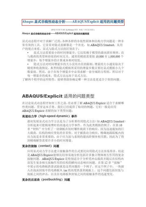
2012-11-14 11:43 by:Abaqus教程来源:广州有道有限元Abaqus显式非线性动态分析——ABAQUS/Explicit适用的问题类型显式动态程序对于求解广泛的、各种各样的非线性固体和结构力学问题是一种非常有效的工具。

它常常对隐式求解器是一个补充，如ABAQUS/Standard；从用户的观点来看，显式与隐式方法的区别在于：•显式方法需要很小的时间增量步，它仅依赖于模型的最高固有频率，而与载荷的类型和持续的时间无关。

通常的模拟需要取10,000至1,000,000个增量步，每个增量步的计算成本相对较低。

•隐式方法对时间增量步的大小没有内在的限制；增量的大小通常取决于精度和收敛情况。

典型的隐式模拟所采用的增量步数目要比显式模拟小几个数量级。

然而，由于在每个增量步中必须求解一套全域的方程组，所以对于每一增量步的成本，隐式方法远高于显式方法。

了解两个程序的这些特性，能够帮助你确定哪一种方法是更适合于你的问题。

ABAQUS/Explicit适用的问题类型在讨论显式动态程序如何工作之前，有必要了解ABAQUS/Explicit适合于求解哪些类问题。

贯穿这本手册，我们已经提供了贴切的例题，它们一般是应用ABAQUS/Explicit求解的如下类型问题：高速动力学（high-speed dynamic）事件最初发展显式动力学方法是为了分析那些用隐式方法（如ABAQUS/Standard）分析起来可能极端费时的高速动力学事件。

作为此类模拟的例子，在第10章“材料”中分析了一块钢板在短时爆炸载荷下的响应。

因为迅速施加的巨大载荷，结构的响应变化的非常快。

对于捕获动力响应，精确地跟踪板内的应力波是非常重要的。

由于应力波与系统的最高阶频率相关联，因此为了得到精确解答需要许多小的时间增量。

复杂的接触（contact）问题应用显式动力学方法建立接触条件的公式要比应用隐式方法容易得多。

结论是ABAQUS/Explicit能够比较容易地分析包括许多独立物体相互作用的复杂接触问题。

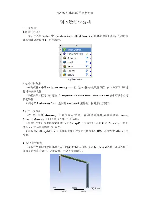
刚体运动学分析一、前处理1.创建分析项目双击主界面Toolbox中的Analysis System>Rigid Dynamics（刚体动力学）选项，在项目管理区创建分析项目A，如图所示。

2.定义材料数据1)双击项目A中的A2栏Engineering Data项，进入材料参数设置界面，在该界面下即可进行材料参数设置。

2)根据实际工程材料的特性，在Properties of Outline Row 2: Structure Steel表中可以修改材料的特性。

3)关闭A2:Engineering Data，返回到Workbench主界面，材料库添加完毕。

3.添加几何模型1)在A2栏的Geometry上单击鼠标右键，在弹出的快捷菜单中选择Import Geometry>Browse，此时会弹出“打开”对话框。

2)在弹出的对话框中选择文件路径，导入chap16几何体文件，此时A2栏Geometry后的？变为√，表示实体模型已经存在。

3)单击DM（DesignModeler）界面右上角的“关闭”按钮退出DM，返回到Workbench主界面。

4. 定义零件行为1)双击主界面项目管理区项目A中的A3栏Model项，进入Mechanical界面，在该界面下即可进行网格的划分、分析设置、结果查看等操作。

2)选择Mechanical界面左侧Outline树结构图中Geometry选项下的所有Solid，在Details of “Solid”中确保所有的Solid对象的Stiffness Behavior（刚度特性）均为Rigid（刚性），如图所示。

5.设置连接1)查看是否生成了Contact接触，如存在，则全部删除，如图所示。

2)选择Mechanical界面左侧Outline树结构图中的Connections对象，然后在工具箱中选择Body-Ground>Revolute，此时树结构图中出现Revolute对象。

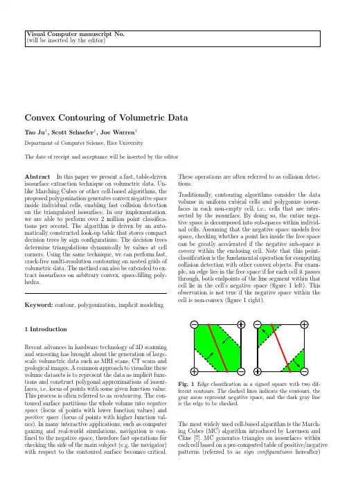
Visual Computer manuscript No.(will be inserted by the editor)Convex Contouring of Volumetric Data Tao Ju1,Scott Schaefer1,Joe Warren1Department of Computer Science,Rice UniversityThe date of receipt and acceptance will be inserted by the editorAbstract In this paper we present a fast,table-driven isosurface extraction technique on volumetric data.Un-like Marching Cubes or other cell-based algorithms,the proposed polygonization generates convex negative space inside individual cells,enabling fast collision detection on the triangulated isosurface.In our implementation, we are able to perform over2million point classifica-tions per second.The algorithm is driven by an auto-matically constructed look-up table that stores compact decision trees by sign configurations.The decision trees determine triangulations dynamically by values at cell ing the same technique,we can perform fast, crack-free multi-resolution contouring on nested grids of volumetric data.The method can also be extended to ex-tract isosurfaces on arbitrary convex,space-filling poly-hedra.Keyword:contour,polygonization,implicit modeling 1IntroductionRecent advances in hardware technology of3D scanning and sensoring has brought about the generation of large-scale volumetric data such as MRI scans,CT scans and geological images.A common approach to visualize these volume datasets is to represent the data as implicit func-tions and construct polygonal approximations of isosur-faces,i.e.locus of points with some given function value. This process is often referred to as contouring.The con-toured surface partitions the whole volume into negative space(locus of points with lower function values)and positive space(locus of points with higher function val-ues).In many interactive applications,such as computer gaming and real-world simulations,navigation is con-fined to the negative space,therefore fast operations for checking the side of the main subject(e.g.the navigator) with respect to the contoured surface becomes critical.These operations are often referred to as collision detec-tions.Traditionally,contouring algorithms consider the data volume in uniform cubical cells and polygonize isosur-faces in each non-empty cell,i.e.,cells that are inter-sected by the isosurface.By doing so,the entire nega-tive space is decomposed into sub-spaces within individ-ual cells.Assuming that the negative space models free space,checking whether a point lies inside the free space can be greatly accelerated if the negative sub-space is convex within the enclosing cell.Note that this point-classification is the fundamental operation for computing collision detection with other convex objects.For exam-ple,an edge lies in the free space if for each cell it passes through,both endpoints of the line segment within that cell lie in the cell’s negative space(figure1left).This observation is not true if the negative space within the cell is non-convex(figure1right).Fig.1Edge classification in a signed square with two dif-ferent contours.The dashed lines indicate the contours,the gray areas represent negative space,and the dark gray lineis the edge to be checked.The most widely used cell-based algorithm is the March-ing Cubes(MC)algorithm introduced by Lorensen and Cline[7].MC generates triangles on isosurfaces within each cell based on a pre-computed table of positive/negative patterns(referred to as sign configurations hereafter)2Tao Ju etal.Fig.2Triangulations from theof cell corners.MC became popular for its fast polygo-nization and easy implementation due to its table-drivenmechanism.However,for some sign configurations,MCdoes not produce polygonizations that are consistentin topology with neighboring cells,and thus result insurface discontinuities[4].This drawback has sparkledextensive research on dis-ambiguation solutions[1],[4],[5],[10]and strategies to generate topologically correctpolygonizations[9].Although these solutions generatetopologically consistent isosurfaces,the resulting nega-tive space inside each cell is sometimes disconnected,andthus not convex.In this paper,we propose a fast table-driven cell-basedcontouring method that generate topologically consis-tent contours,while preserving convexity of the nega-tive space within each cell.The algorithm depends on acomposite look-up table that associates each sign con-figuration with a compact decision tree for dynamic tri-angulation of isosurface patches.The reason for the useof a decision tree is that the actual triangulation de-pends not only on the signs,but also on the magnitudeof corner values.The decision trees are pre-computed toensure a minimal number of tests in determining eachtriangulation.This technique can be extended without difficulty tomulti-resolution contouring.In most multi-resolutionapproaches,direct application of the cell-based contour-ing algorithm to a grid of non-uniform cells can resultin surface cracks,i.e.discontinuity between iso-surfacesgenerated from neighboring cells at different resolutions.Various multi-resolution frameworks have been proposedfor contouring on non-uniform grids[3],[8],[11],[12],[14],yet they involve special crack-patching strategies.Bloomenthal[2]proposes an adaptive contouring methodwhich requires run-time face tracing to maintain con-sistent contours for neighboring cells.We show that byconstructing look-up tables for transition cells using theabove algorithms,the same table-driven contouring methodcan be applied to non-uniform data to generate crack-free isosurfaces.The remainder of this paper is organized as follows.Afterreviewing the table-driven Marching Cubes algrorithm,we present the convex contouring algorithm on uniformgrids.Then we explain the automatic construction oflook-up tables in more detail.Next we extend the pro-posed technique to non-uniform grids to produce crack-free contour surfaces.We conclude by discussing otherpossible extensions and applications.2Marching Cubes and Look-up TablesMarching Cubes is a popular algorithm for extractinga polygonal contour from volumetric data sampled ona uniform3D grid.For each cell on the grid,the edgesintersected with the iso-surface are detected from signsat cell corners.The algorithm then forms triangles byconnecting intersections on those edges(referred to asedge intersections hereafter).To speed up the process,ituses a look-up table that establishes triangulations foreach sign configuration.Since there are8corners in acell,the look-up table contains256entries,four of whichare shown infigure2.Using the look-up table,the Marching Cubes algorithmcontours a cell in two steps:1.Look up the triangulation in the table by the signconfiguration,2.For each triangle,compute the exact location of eachvertex(edge intersection)from values at the cell cor-ners by linear interpolation.The Marching Cubes algorithm is fast because it uses ta-ble look-up to build polygonal contours.Unfortunately,the contoured surface generated by the original look-uptable in[7]may contain holes,since the triangular con-tour within each cell is not always consistent with thatof the neighboring cells(figure3).Although this problem wasfixed in later work,it re-veals another drawback of manually created tables.Theentries in the Marching Cubes’look-up table are con-structed by identifying15topologically distinct sign con-figurations and triangulating each case by hand.The lackof automation makes it susceptible to errors and diffi-cult to adapt to other polyhedrons.As we shall see,thelook-up tables used in convex contouring are constructedalgorithmically based on the topology and geometry ofgiven polyhedrons,and therefore minimizes possible er-rors.Convex3Fig.3Two the Marching Cubes topology.3Convex Contouring Using Look-up Tables The goal of convex contouring is to extract polygonal contours that enclose convex negative spaces within each cell.In this section,we will introduce the concept of con-vex contours and describe the proposed polygonization technique based on a pre-computed look-up table.Ex-amples of convex contouring will be presented together with performance comparison with the Marching Cubes algorithm.3.1Convex contourAssuming that the underlying implicit function is trilin-ear inside each cell,the convex hull of the negative space in a cell is the convex hull of all negative cell corners and edge intersections.The convex contour is the part of this convex hull that lies interior to the cell.In 2D,for exam-ple,the convex contour consists of interior line segments connecting edge intersections (i.e.,dashed lines in fig-ure 1left).In 3D,the convex contour consists of interior triangles whose vertices are edge intersections (figure 4left).Together with the triangles that fill the negative regions on cell faces (figure 4right),they constitute the convex hull of the negative space inside thecell.Fig.4Convex contour on the convex hull of the negative space.Note that the convex contour in a cell is outlined by linear convex contours on the faces of the cell (high-lighted in figure 4).Since the linear convex contour in a2D square is uniquely determined given the signs at the 4corners (allowing movement of the edge intersections along the edges),the polygonal convex contours from neighboring 3D cells always share the same linear con-tour on the common face.Hence convex contours always form topologically consistent isosurfaces.In figure 5,we show the convex contours for the same cells from figure 2.In comparison,we observe that the convex contour always encloses a connected,convex neg-ative space within the cell,whereas the contour from the Marching Cubes algorithm does not.Note that a convex contour is sometimes composed of multiple connected components,as shown in the rightmost cell of figure 5.Each of these connected piece of the contour is called a patch ,which may contain multiple holes (such as the center left cell in figure 5).Each hole on the patch is surrounded by a ring of linear convex contours that can be detected by the signs at the corners.Hence a look-up table for patch boundaries can be constructed automat-ically for each sign configuration.3.2Triangulation and Decision treesUnfortunately,although the boundary of the patches on the convex contour is unique for each sign configuration,the actual polygonization is not.In fact,different scalar values at cell corners,which determine the location of edge intersections,may modify the shape of the convex hull and result in different triangulation of the convex contour.As illustrated in figure 6,two cells that share the same sign configuration,but with different scalars at cell corners,result in different triangulated convexcontours.Fig.6Triangulation in cells with different scalar values at corners.Edge intersections are indicted by gray dots.To determine the correct triangulation based on the lo-cation of edge intersections,one could apply a full-scale convex-hull algorithm to compute the convex hull of the negative space.However,such algorithms are too gen-eral for our purposes,since we want only the part of this convex hull that lies interior to the cell.Instead,we can take advantage of the fact that the topology of the boundary is known for each patch on the convex contour.In fact,we can construct a set S of all possible triangu-lations for each patch.For example,figure 6shows the4Tao Ju etal.Fig.5Convex contours in cells withonly two possible triangulations for the convex contour ofthat sign configuration,since the contour contains a sin-gle4-sided patch.According to Euler’s polygon divisionproblem[6],there are(2n−4)!(n−1)!(n−2)!ways to triangulate an−sided patch into n−2triangles.In fact,this size ofS can be further reduced if we realize that the verticesof these triangles are restricted tofixed cell edges,hencesome triangulations will never appear on the convex hullof negative space.We will discuss this process in detailwhen we describe how the look-up table is constructed.Now we can think of the triangulation problem as thefollowing:given the exact locations of the edge inter-sections,choose an appropriate triangulation from S sothat the triangles satisfy the convex hull property(i.e.,all edge intersections and negative corners lie on one sideof the triangle).Hence we need a fast method to differ-entiate the correct triangulation from others by lookingat the edge intersections.Assuming that triangles on theconvex contour face inside the convex hull of the nega-tive space,we can do this by the following4-point test:given four distinct edge intersections V1,V2,V3,V4,if V4lies on the front-facing side of the triangle(V1,V2,V3),then the inverted triangle(V1,V3,V2)does not belongto the convex contour(figure7left).Similarly,triangles(V1,V2,V4),(V2,V3,V4)and(V3,V1,V4)do not satisfythe convex hull property.Otherwise,by symmetry,weclaim that triangles(V1,V2,V3),(V1,V4,V2),(V2,V4,V3)and(V1,V3,V4)do not lie on the convex contour(figure7right).Note that if all vertices lie on the same plane,either choice can be made.V1V2V3V4V1V2V3V4Fig.7Four-point test with vertices V1,V2,V3,V4.Each4-point test on the edge intersections rules outthose from the set S of all possible triangulations thatcontain any of the four back-facing triangles.Since anytwo triangulations differ at least in the triangles sharedby one of the boundary edge,the correct triangulationcan be distinguished from every other triangulation in Sthrough appropriate4-point tests.For best performance,a decision tree can be built to distinguish each triangula-tion through a minimal set of tests.An example of sucha decision tree is shown infigure8for a5-sided patch.At each node,the remaining triangulations are shownand the4-point test is represented by indices of the fourvertices(the order is shown at the top left corner).If thefourth vertex lies on the front-facing side of the triangleformed by thefirst three vertices(in order),we take theleft branch.Otherwise,we follow the right branch.Theprocess stops at a leaf node,where a single triangulationisleft.2,4,5,13,4,5,12,3,4,52,3,5,11,2,3,412345Fig.8A decision tree using4-point test for5-sided patches.Since the construction of decision trees is based on theoriginal set S,they can be pre-computed and optimizedfor every patch in each sign configuration.As we shallsee,the maximum depth of all these decision trees is5and the average tree depth is1.88.In other words,thecorrect triangulation of the convex contour in a cubic cellcan be determined by performing a maximum of5point-face trials on the edge intersections,and on average nomore than2trials.3.3The look-up tableThe look-up table contains256entries,one for each signconfiguration of a cubic cell.In each entry,the look-uptable stores the decision trees computed for each patchConvex Contouring of Volumetric Data5 Fig.9Two screen shots of a real-time navigation application using a convexly contoured terrain.by traversing the nodes in the decision trees in pre-order. Each non-leaf node contains a4-point test,and each leaf node stores a triangulation.The edge intersections in4-point tests and triangulations are represented by indices of the edges on which they lie.Two example entries in this table are shown in table1,with their correspond-ing sign configurations and edge indexing drawn on the right.3.4Contouring by table look-upsIn comparison with the Marching Cubes algorithm,con-vex contouring extracts the polygonal contour in a cell in two steps:1.Look up the decision trees(one for each patch)in thetable by the signs at the cell corners,2.For each decision tree,perform4-point tests on spec-ified edge intersections until arriving at a single tri-angulation.Fig.10Convex contouring on volumetric data.Infigure10,two sets of volumetric data generated by scan-conversion of polygonal models are contoured us-ing the new method.Observe that the edges on the sur-face are manifold and the contour is crack-less.Since the negative space inside each non-empty cell is convex, collision detection can be localized into cells and there-fore become independent of the grid size.Figure9shows two screen shots of a real-time navigation program in which the movement of the viewer is confined within the negative space.The terrain is an iso-surface constructed using convex contouring on a256cubic grid.On a con-sumer level PC machine(dual1.5GHz processors with 2.5G memory),we achieved over2million point classifi-cations per second.As we mentioned before,the average number of tests used to determine triangulation for each patch is less than2.Hence we can perform convex contouring on vol-umetric data with speed comparable to the Marching Cubes algorithm.In table2,the performance of con-vex contouring is compared with that of the Marching Cubes for contouring the terrain infigure9on differ-ent grid sizes.We also compared the average number of triangles generated in each cell in both methods.Notice that convex contouring generates on average only about 2%more triangles than the Marching Cubes algorithm. These extra triangles are needed to preserve the convex-ity of the negative space.Grid Size Marching Cubes Convex Contouring 1283125ms141ms2563781ms907ms51232109ms2437msAvg.Triangles 3.181 3.257Table2Comparison of total contouring time and average number of triangles per cell in convex contouring and the Marching Cubes.6Tao Ju et al.Index Table Entry Cell Configuration171{1,9,12,7}→4-point test{{1,9,7},{9,12,7}}→Triangulation{{1,9,12},{1,12,7}}123456789101112125{1,3,6,12}→4-point test in parent node{1,12,10,2}→4-point test in left child{{1,3,12},{1,12,2},{3,6,12},{12,10,2}}{{1,3,12},{1,12,10},{1,10,2},{3,6,12}}{1,12,10,2}→4-point test in right child{{1,3,6},{1,6,12},{1,12,2},{12,10,2}}{{1,3,6},{1,6,12},{1,12,10},{1,10,2}}123456789101112Table1Two example entries in the look-up table.Each entry is a list of triangulations(each stored as a list of triangles) and4-point tests(each stored by the indices of the vertices)traversed from the decision tree in pre-roder.4Automatic Construction of Look-up TablesIn this section,we will review the table construction pro-cess in more detail.For a given sign configuration,we first detect the patch boundaries as a group of rings of linear contours.Then,for each patch,we construct the set of all possible triangulations that could take place on the convex hull of the negative space.Finally,an opti-mal decision tree is built for every patch detected on the contour.The look-up table can be found on the web at /jutao/research/contour tables/.4.1Detection of patch boundariesA patch on the convex contour in a cubic cell is bounded by linear convex contours on cell faces.These linear con-tours form single or multiple rings that surround the ”holes”of the patch.Since the linear convex contours are unique on each cell face for a given sign configura-tion,a single ring can be constructed using the following tracing strategy:starting from a cell edge that exhibits a sign change(where an edge intersection is expected) and facing the positive end,look for the next edge with a sign change by turning counter-clockwise on the face boundary.Repeat the search process until it returns to the starting edge,when a closed ring is formed(seefigure 11).Notice that face-tracing produces oriented linear convex contours on each cell face.Each linear contour on the cell face is directed so that the negative region on that face lies to its left when looking from outside.There-fore the triangles on the convex contour of the cell that share these linear contours will face towards the nega-tive space.The orientation of the rings are importantfor linear contours already built,and dashed arrows indicate the tracing route.determining the set of possible triangulations that share the same patch boundary.Similar tracing techniques have been described by nu-merous authors in[2],[9],[13],in which convexity of the negative region on each cell face is preserved.These algo-rithms construct a single ring for each patch boundary. However,the problem remains on how to group multiple rings to form the boundary of a multiple-genus patch (such as the center left cell infigure5).Although such patches arise in only4cases among256sign configura-tions,they may appear much more often in other non-cubic cells(such as transition cells in multi-resolution grids,see Section6).We need to be able to identify these cases automatically from the sign configuration and group the rings appropriately.By definition,a patch is a continuous piece on the con-vex hull of negative space.Hence it also projects onto a continuous piece of regions on the cell faces.These regions are positive areas that surround positive cor-Convex Contouring of Volumetric Data7ners connected by cell edges.Therefore the boundary of each patch on the convex contour isolates a group of positive corners that are inter-connected by cell edges. The previous face-tracing algorithm could be modified so that rings constructed around a same edge-connected component of positive corners are grouped to form the boundary of a single patch.This rule is demonstrated in figure12.In the top left cell,two rings of linear contours form the boundary of two patches,due to the presence of two isolated positive corners.In the top right cell,where there is only one edge-connected component of positive corners,the two rings are grouped to form the bound-ary of a single cylinder-like patch.The connectivity of the positive corners in these two cells are illustrated at the bottom offigure12.In contrast,face-tracing without ring-grouping would give the same result in both cells, thus violating the convex hull property in the secondcell.Fig.lighted)to form boundaries of patches.Positive corners are colored gray.Bottom:Connectivity graph of positive corners 4.2Pre-triangulation of Convex ContourThe set of possible triangulations for a patch with an oriented boundary topology can be enumerated by re-cursive algorithms.However,this often results in redun-dant triangulations that never appear on the convex con-tour.For example,the genus-2patch in the center left cell infigure5can be triangulated in only one way on the convex hull of the negative space,regardless of the magnitudes of scalar values at the corners.In contrast, brute-force enumeration would return21possible trian-gulations for an arbitrary genus-2patch with two trian-gular holes.The key observation is that,the patches on the convex contour are not arbitrary patches,their ver-tices(edge intersections)are restricted tofixed edges on the cell.These spacial restrictions limit the number of possible triangulations that could occur on the convex contour.For fast polygonization at run-time,we hope to pre-triangulate each patch as much as possible during table construction,based only on the sign configuration. By the convex hull property,the half-space on the front-facing side of a triangle on the convex contour must con-tain(or partially contain)every other cell edge that ex-hibits a sign change.Note that the three vertices of the triangle can move only along threefixed cell edges,this half-space is always contained in the union of the half-spaces formed when the three vertices are at the ends of their cell edges.Hence we have a way to identify triangles that will not appear on the convex contour:given three cell edges(C1,C2),(C3,C4)and(C5,C6)(C i are cell cor-ners),construct border triangles,i.e.,triangles formed by one end of each edge in order(such as(C1,C3,C5)).If there is an edge on the cell exhibiting a sign change that lies completely to the back of all non-degenerate border triangles,any triangle whose vertices belong to these three edges(in order)will not lie on the convex con-tour.This idea is illustrated infigure13.The highlighted cell edge on the left exhibits a sign change,and lies to the back of all the border triangles constructed from the three dashed edges(E1,E2,E3).Hence the dashed trian-gle formed by intersections on those edges never appears on the convex contour.In contrast,the highlighted cell edge on the right lies partially to the front of at least one of the border triangles formed by the edges(E1,E2,E3), hence the dashed triangle may exist in the triangulation of the convex contour.E1E2E3E1E2E3Fig.13Identifying triangles that do not lie on the convex contour.By eliminating triangulations that contain these ineli-gible triangles,we can trim down the space of possible triangulations.For example,the number of remaining triangulations for thefirst three cells infigure5are re-spectively4,1and4.4.3Construction of decision treesEven after pre-triangulation,some patches still have many potential triangulations on the convex hull of the nega-tive space.To speed up the polygonization at run-time,8Tao Ju et al.we can pre-compute a set of4-point tests on the vertices of the patch(edge intersections)to distinguish between the remaining triangulations.These tests can be orga-nized in a decision tree structure,introduced in the last section.Different sets of tests result in differently shaped decision trees.To obtain optimal performance,we imple-ment a search algorithm that looks for the optimal set of tests that produces a decision tree with the small-est depth.Since each of the two outcomes of a single test eliminates a non-intersecting subset of the remain-ing triangulations,the minimal depth of the correspond-ing decision tree is lower bounded by log2N,where N is the total number of triangulations.For example,the depth of an optimized decision tree for a patch of length 4,5and6are1,3and5respectively.Further computa-tion reveals that the maximum length of a patch(which can not be pre-triangulated)in a cubic cell is6;hence any patch can be triangulated within5point-face trials on thefly by walking down the pre-computed decision tree.On average,however,it only takes1.88tests to de-termine the triangulation of a patch,due to infrequent occurrence of large patches and the reduced triangula-tion space as a result of pre-triangulation.5Multi-resolution Convex ContouringIn volume visualization,the number of polygons gener-ated by uniform contouring easily exceeds the capacity of modern hardware.For real-time applications,it is often advantageous to display the geometry at different lev-els of detail depending on the distance from the viewer. This technique has the advantage that it speeds up the rendering process without sacrificing much visual accu-racy.By using a view-dependent approach,the grid is contoured at different resolutions depending on the dis-tance from the navigator.In particular,we can create a series of nested bounding boxes centered at the viewer, with the grid resolution decreasing by a factor of2.A2D example of this multi-resolution framework is shown infigure14left,in which a circle is contoured using cell grid at two different resolutions.When the coarse cells at the top meet thefine cells at the bottom,the con-tour in the coarse cells need to be consistent with the contour from the neighboringfine cells on the common edges.We call these coarse cells transition cells,which are adjacent to cells at afiner resolution.A2D transition cell thus hasfive corners andfive edges,as shown in the middle offigure14.By connecting edge intersections on each cell edge,the transition cells can be contoured in a way similar to a regular4-corner cell,yielding consistent contours with the adjacentfine cells.Some of the con-toured example are shown infigure14right.Notice that the convexity of the negative region is still preserved in each transition cell.In3D,a transition cell between two resolutions is either adjacent to twofine cells on an edge,or adjacent to four fine cells on a face(seefigure15left).These two types of cells can be regarded as convex polyhedrons with9 corners(figure15center)and13corners(figure15right) respectively.Since the previous discussion on regular cells applies to any convex polyhedron,we can also build look-up ta-bles and perform convex contouring on these transition cells.In this way,crack-free surfaces can be contoured on nested grids within the same framework as uniform contouring.5.1Convex contours in transition cellsAs in a regular cell,the convex contour inside a tran-sition cell is outlined by the linear contours on the cell faces.Since the linear convex contour is unique on each face for a given sign configuration,the boundary of patches on the convex contour can be pre-computed using the proposed face-tracing algorithm.At the top offigure16, the oriented boundaries of patches in different transition cells are detected and drawn as dashed arrows.Since con-vex contours from neighboring cells in a multi-resolution grid always share the same linear contour on the com-mon face as their boundaries,topological consistency is preserved everywhere on the contouredsurface.Fig.16Patch boundaries(top)and triangulation(bottom) in three transition cells.By pre-computing optimal decision trees for each patch, the triangulation can be determined by applying succes-sive4-point tests on the edge intersections.At the bot-tom offigure16,patches detected from the cells on the top are triangulated on the convex hull of the negative space.However,due to the presence of four co-planar faces on a13-corner cell,this convex hull could degener-ate onto a plane(figure17left).To determine the correct triangulation of the convex contour on the degenerate convex hull,we introduce an outward perturbation to。

2021年2月第2期Vol. 42 No. 2 2021小型微型计算机系统Journal of Chinese Computer Systems一种自适应运动目标检测算法及其应用李善超，车国霖，张果,杨晓洪(昆明理工大学信息工程与自动化学院，昆明650500)E-mail ：991186428@ qq. com摘要：针对ViBe 算法在动态背景下存在鬼影消除时间长、算法适应性差、前景检测噪声多的问题，本文提出一种基于ViBe 算法框架的改进算法.该算法釆用鬼影检测法标记第1帧中的鬼影区域，并向位于鬼影区域的背景模型中强制引入背景样本，从而快速抑制鬼影；在像素分类过程中，引入自适应分类阈值，解决全局阈值易受动态噪声干扰的问题；在背景模型更新中，根 据像素分类的匹配值来动态决定更新因子，提高算法适应场景变化的能力.定性与定量的对比实验结果表明，本文算法相较于ViBe 算法能够有效地检测动态背景下的运动目标，应用于河流漂浮物检测场景中也有较好的效果.关键词：ViBe ；动态背景;运动目标检测；自适应方法;河流漂浮物检测中图分类号：TP391文献标识码:A 文章编号：1000-1220(2021)02-0381-06Adaptive Moving Target Detection Algorithm and Its ApplicationLI Shan-chao ,CHE Guo-lin ,ZHANG Guo,YANG Xiao-hong(Faculty of Information Engineering and Automation ,Kunming University of Science and Technology ,Kunming 650500,China)Abstract : Aiming at the problem that ViBe algorithm has long ghost elimination time , poor algorithm adaptability and high foreground detection noise in dynamic background , this paper proposes an improved algorithm based on ViBe algorithm framework. The algorithmuses the ghost detection method to mark the ghost region in the first frame , and forces the background sample into the background model in the ghost region to quickly suppress the ghost. In the pixel classification process , the adaptive classification threshold is intro ・ duced to solve the problem that the global threshold is susceptible by dynamic noise interference. In the background model update , theupdate factor is dynamically determined according to the matching number of the pixel classification to improve the algorithm's abilityto adapt to scene changes. The comparison experimental results of qualitative and quantitative shows that the algorithm in this paper can effectively detect moving targets in dynamic background compared to the ViBe algorithm , and it also has a better effect in the de ­tection of river floating objects.Key words : ViBe ； dynamic background ； moving target detection ； adaptive method ； river floating debris1引言运动目标检测在智能视频监控的应用中扮演着重要的角 色，是计算机视觉领域的一个研究热点⑴•运动目标检测的 实质是在视频序列中定位运动中的目标，而准确的前景检测 是目标分类、目标跟踪和行为识别研究的重要基石⑺叫运动目标检测算法按类别可分为帧差法⑴、光流法⑷、背景建模 法"向3种.帧差法原理简单且易于设计，然而其检测结果存 在空洞和鬼影的问题.光流法虽然精度高，但由于其计算量大，不适用于对实时性有较高要求的场景.背景建模法是在初 始化过程中构建出由背景样本组成的模型，并将当前帧与背 景模型进行差分，从而对像素进行分类,最后得到运动目标.其具有精度高实时性好的特点.背景模型的准确性决定了背景建模法的检测精度，主要影响检测精度的因素有鬼影问题、 动态背景、噪声干扰等⑴.高斯混合模型(GMM ,Gaussian mixture model)[8]是运动目标检测算法中最为经典的算法，其本质是基于像素样本统 计信息的背景建模方法，能够对复杂背景进行准确建模，然而 其计算复杂度较高GMG 算法切是统计背景模型的概率，采 用贝叶斯逐像素分割，但在动态场景中其检测精确度较低.核 密度估计算法(KDE,Kernel Density Estimation)[10]是一种非 参数背景建模方法，其通过大量的背景样本估算背景像素的概率密度函数，从而根据像素背景概率来分类像素，然而其内 存占用与计算复杂度都较高.Bamich 等人⑴•切于2009年提出一种非参数化视频背景提取算法(ViBe , Visual BackgroundExtractor),该算法是为每个像素设置一个样本集，并与新帧像素进行阈值比较,从而对像素进行分类,其具有实时性好、鲁棒性高和易于集成于嵌入式设备的特点.然而ViBe 算法仍 存在一些不足，限制了其在动态场景中的应用.例如：1)当初 始化图像中存在运动中的目标时,ViBe 算法会在后续帧中检 测到鬼影，降低了算法的检测精度且鬼影消除时间长；2)ViBe 算法在动态场景中检测精度低，容易受动态噪声干扰;3) ViBe 算法的背景模型更新策略无法适应背景动态的变化.针对ViBe 算法存在的问题,本文提出一种自适应运动目收稿日^:2020-03-06 收修改稿日期：202045-11基金项目：国家重点研发计划项目(2017YFB0306405)资助；国家自然科学基金项目 (61364008)资助.作者简介：李善超，男，1994年生，硕士研究生，研究方向为数字图像处理；车国霖，男,1975年生，硕士，副教授，研究方向为 智能控制；张 果，男，1976年生，博士，副教授，研究方向为智能測控;杨晓洪，女,1964年生，高级工程师，研究方向为综合自动化.382小型微型计算机系统2021年标检测算法.本文将从以下3个方面对ViBe算法进行改进.1)采用鬼影检测法标记鬼影区域并强制引入背景样本，加速鬼影的抑制;2)采用自适应匹配阈值的方法进行像素分类，提高算法抗干扰的能力;3)根据像素分类的匹配值动态调整更新因子，提高算法适应场景变化的能力.本文采用CDNET 数据集中dynamicBackground视频类中的5个视频序列和3组河流漂浮物的视频序列进行研究，以本文算法和其他5种算法为例，定性、定量对实验结果做出质量评价和分析.研究结果表明，本文算法相较于ViBe算法在召回率、精确率和F 度量值方面均有提高，错误分类比更低,达到了预期的目标.2ViBe算法原理ViBe算法是基于样本随机聚类的背景建模算法，具有运算效率高、易于设计、易于集成嵌入设备的特点，能够实现快速的背景建模和运动目标检测.算法的步骤包括背景模型初始化、像素分类过程和背景模型更新.2.1背景模型初始化1)背景模型定义:ViBe算法的背景模型是由N个背景样本组成的,v(x)是像素x的像素值，则背景模型M(x)定义如公式(1)所示：=|Vj(x),v2(x),v N(x)|(1)2)背景模型初始化:ViBe算法利用视频序列第1帧建立背景模型，从第2帧开始算法就可以有效地检测运动目标.背景模型初始化是在像素x的8邻域Nc(x)中选取一个像素值作为背景样本，重复N次,如公式(2)所示：(N g(x)=Ui,¾,--,¾IJ(2)〔M(x)=1v(ylyeN c(x))I3)随机选取策略:背景建模时，背景样本始终采用随机选取邻域像素的策略，以使背景模型更加稳定可靠.2.2像素分类过程ViBe算法采用计算欧氏距离来进行像素的分类. S”(v(x))是以像素值v(x)作中心，匹配阈值R为半径的二维欧氏空间，若v(x))与M(x)的交集H{•}中元素个数不小于最小匹配数则认为像素x是背景像素，如公式(3)所示:H{Sx(v(x))n I V,(x),v2(x),—,v w(x)I I(3) 2.3背景模型更新1)保守更新机制:ViBe算法通过保守更新机制进行背景模型更新，即如果像素被分类为背景像素，则以i/e(e是更新因子)的概率替代背景模型中的任一样本.假设时间是连续且选择过程是无记忆性的，在任一dt时间后，背景模型的样本随时间变化的概率如公式(4)所示：P(t,t+dt)=e-1"(^)d,(4)公式(4)表明，背景模型样本值的预期剩余寿命都呈指数衰减，背景模型的样本更新与时间无关.2)随机更新机制:ViBe算法通过随机更新机制进行样本替换,使得每个样本的存在时间成平滑指数衰减，提高了算法适应背景变化的能力，避免了旧像素长期不更新带来的模型劣化的问题.3)空间传播机制:ViBe算法也将背景像素引入邻域的背景模型中，保证了邻域像素空间的一致性.例如，用背景像素替换任一邻域(x)中的任一样本.ViBe算法首次将随机聚类技术应用于运动目标检测中，使得算法在背景模型初始化、像素分类过程、背景模型更新3个方面都比较简单,保证了算法的实时性，因此ViBe算法被广泛应用于现实生活中3提出的改进算法ViBe算法采用随机采样、非参数化和无记忆的更新策略，使得其具有较好的性能，但其在动态场景下仍然存在不能快速抑制鬼影、难以消除动态噪声以及无法适应场景动态变化的问题,本文将从以下3个方面对ViBe算法进行改进.3.1鬼影检测ViBe算法利用第1帧建立背景模型，但也不可避免的将第1帧中存在的运动目标前景像素引入到背景模型中，导致鬼影问题和彫响算法的检测精度.假设背景模型M(x)是由第1帧中的前景像素样本f(x)组成的，当运动目标离开时，ZU)不在背景像素值b(x)的S”(b(x))圆内，背景像素被错误的分类为前景,如公式(5)所示,则在第1帧中运动目标所在的区域就会出现虚拟的前景(鬼影).rM(x)=|/；(x)J2(x)，―J N(x)}(s&(x))nM(x)=0本文针对这一问题，应用鬼影检测法标记出第1帧中的鬼影区域,并向位于鬼影区域的背景模型中强制引入背景样本，减少其中前景像素的数量，从而快速抑制鬼影.鬼影检测法借鉴了帧间差分法并对其进行改进,其原理是提取视频序列的前3帧图像，第1帧图像分别与后两帧图像做差分运算，设定差分阈值并对差分后的图像进行二值化分类,将二值化结果做逻辑或操作和形态学操作，即得到标记有第1帧运动目标的鬼影模板Ghost(x),在鬼影模板Ghost(x)中大于0的位置是第1帧中鬼影区域的.具体定义如公式(6)、公式(7)和公式(8)所示：if I厶(x)-厶+|(兀)I>Tif\IM一人+|(x)lwTM)={o-/“2(x)IWTGhost(x)=£>i(x)or D2(x)(6)(7)(8)式中：D(x)为二值化图像，人(x)为第R帧输入图像，一般A=1为图像差分阈值，。

I.J.Modern Education and Computer Science, 2013, 5, 60-65Published Online June 2013 in MECS (/)DOI: 10.5815/ijmecs.2013.05.07Activity Recognition with Multi-tape FuzzyFinite AutomataH. Karamath AliAssociate Professor in Computer Science, Periyar EVR College (Autonomous), Tiruchirappalli, IndiaEmail: hkaramath@Dr. D. I. George AmalarethinamAssociate Professor & Director-MCA, Jamal Mohamed College (Autonomous), Tiruchirappalli, IndiaEmail: di_george@Abstract— Recognizing the activities performed by the user in an unobtrusive manner is one of the important requisites of pervasive computing. Users perform a number of activities during their day to day life. Tracking and deciding what a user is doing at a given time involves a number of challenges. The lack of a precise pattern in doing an activity at different times is one among them. The number, order, and duration of the different steps involved in an activity vary significantly, even when the activity is done by the same user at different times. To overcome these challenges, a number of simultaneous inputs have to be handled with provisions for handling variations in number, order and duration of these inputs. This paper explains how multi-tape fuzzy finite state automata can be used to effectively recognize human activities. The method explained is found to give good results when tested using publicly available activity datasets collected in a smart home environment.Index Terms —Pervasive Computing, Activity Recognition, Fuzzy AutomataI.I NTRODUCTIONThe ability to recognize human activities automatically and unobtrusively in a smart environment has a number of applications varying from essential services such as healthcare and security to luxurious services such as automatically adjusting room ambience and ergonomics[1][2][3]. A smart environment usually has a large number of different types of sensors embedded in almost every possible component of the environment. These sensors provide input about the user’s interaction with the environment. Using these inputs the activity recognition system has to decide and possibly predict the activity performed by the user. This decision or prediction may then be used by some other larger system to provide appropriate services to the user. The task of activity recognition gets complicated by the need to handle many simultaneous sensor inputs and the impreciseness with which users perform activities. A number of probabilistic and structural methods have been developed by researchers to recognize activities [4] - [19]. This paper illustrates how multi-tape fuzzy finite automata can be used for recognizing human activities. The multi-tape feature will be useful in representing multiple simultaneous inputs; and the concept of fuzziness can be used to represent and deal with the variations in the pattern of human activities. The method is found to produce results that are comparable to other frequently used methods.The remainder of this paper is organized as follows: Section II presents an overview of the related works in activity recognition; section III defines the problem statement; section IV presents the fundamental concepts of multi-tape automata and fuzzy automata; section V explains the proposed method; section VI discusses the dataset used and the experiment conducted; and section VII presents conclusion.II.RELATED WORKIn their attempt to develop a framework for solving the problem of activity recognition, researchers have used a number of models. Among them, the Hidden Markov Model (HMM) is the most commonly used. Sanchez, D. et al. [1] trained a discrete HMM to map contextual information to a user activity. The model was trained and evaluated using data captured from 200 hours of detailed observation and documentation of hospital workers. Tim van Kasteren et al. [2] recorded a dataset consisting of 28 days of sensor data in a smart home environment and through a number of experiments showed how the HMMs perform in recognizing activities. An approach for multi-person activity recognition in an office environment using audio as well as video features, employing a multilevel HMM framework is used by Christian Wojek et al. [3]. Human activities embedded in video sequences acquiredin an archeological site are automatically recognized using Discrete HMMs by Marco Leo, et al. [4]. Weiyao Huang, et al. [5] used Discrete HMM for human posture training, modeling and activity matching to recognize human motion. Other HMM variations such as Coupled HMM, Fuzzy HMM, Hierarchical HMM and Reconfigurable HMM are used by other researchers [6] [7] [8] [9].RocíoDíaz de León et al.[10] used a Bayesian network for recognition of continuous activities, by considering the direction change between frames to track the motion of several limbs and to recognize different activities. An approach for human activity recognition that can recognize activities performed at different velocities by different people and can work with missing data, based on the Fourier transform and Bayesian networks was presented by RocíoDíaz de León [11]. A system that uses naïve Bayesian classifier for recognizing activities in the home setting using a set of small and simple state-change sensors is introduced by E.M. Tapia, et al. [12]. In the framework suggested by Sangho Park and J.K. Aggarwal [13], human action is represented in terms of verbal description according to subject + verb + object syntax, and human interaction is represented in terms of cause + effect semantics between the human actions. Then, a dynamic Bayesian network is constructed to estimate temporal evolution of the human actions for recognizing the dynamic gestures of the body parts. Tim van Kasteren and Ben Kr¨ose [14] used a Dynamic Bayesian Network, to model the temporal aspects of the activities of daily living (ADL) of elders. They observed that adding more sensors does not necessarily increase accuracy. A multi-level dynamic Bayesian network was used to perform complex event recognition by Justin Muncaster and Yunqian Ma [15]. The levels of the network are used to enforce state hierarchy while the lowest level models the duration of simplest event. The probability that a scenario occurs is computed from the mobile object properties obtained from a sequence of image frames using several layers of naive Bayesian classifiers in the work presented by Somboon Hongeng, et al. [16]. Friedrich Steimann and Klaus-Peter Adlassnig presented a framework for an intelligent bedside monitor that derived an abstraction of the current status of a patient by fuzzy state transitions on pre-processed input supplied continuously by clinical instrumentation [17]. This is one of the earlier works that use fuzzy automata for activity recognition. A Fuzzy Rule based Classifier and two Fuzzy Finite State Machines (FFSM) are used by A. Alvarez-Alvarez, et al.[18] to recognize activities like working in the desk room, crossing the corridor, having a meeting, etc. The classifier is used to get an approximate position at the level of discrete zones such as office, corridor and meeting room. One of the FFSM is used for human body posture recognition and the other FFSM combines the localization and posture recognition. The use of fuzzy finite state systems is demonstrated in [19] for human gait modeling. Gonzalo Bailador and Gracián Triviòo [20] propose a syntactic pattern recognition approach based on fuzzy automata, which can cope with the variability of patterns by defining imprecise models. The approach is called temporal fuzzy automata as it allows the inclusion of time restrictions to model the duration of the different states. This approach is used for recognizing hand gestures.Though the above works use fuzzy automaton to deal with variability and impreciseness of human activities, the states of the fuzzy automata are manually defined by an expert. This will be tedious, as the number of states becomes very large. So in this paper we propose to use an algorithm suggested by Henning Fernau [21] to automatically construct a DFA to recognize human activities using a set of sensor inputs, represented as strings. Then the concept of fuzziness is introduced by using appropriate functions to deal with variability and impreciseness of human activities. The proposed method is tested with a publicly available data set, and the results are comparable to other commonly used methods.Figure 1.Sensor readings and activity labelsIII. T HE P ROBLEMThe objective is to recognize activities from sensor readings in a smart environment. For this, the time series data of sensor readings is divided into time slices of constant length. Each time slice is labeled with the activity performed during that time slice [2]. A vectoris used to represent the sensor readings at time slice, where represents the input from the sensor during the time slice and ‘N’ is the number of sensors. The activity performed during time slice ‘’ is represented by. So, the task of the activity recognition system is to find an association between a sequence of observation vectors x={} and a sequence of activity labels y={12n}. Fig.1 illustrates the above setup, with Δt representing a timeslice.IV. M ULTI-TAPE FINITE AUTOMATAA two-way finite-state automaton with tapes scans n read-only input tapes, each with an independent head [22]. At every step, the transition function determines the possible next states and head movements, based on the current state and the symbols currently under each head. Two special symbols, respectively mark the left and right ends of each input tape;denotes the extended alphabet.Figure 2.Time Slices and States Definition: A two-way nondeterministic finite-state automaton with n tapes is a tuple (∑, , δ, q0, F), where : ∑ -- is the input alphabet, such that , ∑;– is the finite set of states;δ: is the transition function that maps current state and input to a set of next states and head movement directions, with the restriction that the head does not move beyond the end markers;is the initial state;F a subset of , is the set of accepting states.The configuration of a two-way nondeterministic finite-state automaton , is defined as a (2n+1)-tuple,where is the current state, and, for is the content of the k-th tape and is the position of the k-th head; when (resp.) the head is on the left marker (resp. right marker ).The transition relation between configurations is definedas:if and only if, for each is the symbol at position in input wordincludes a tuple and for each .A run of on input is a sequence of configurations such thatand for all . A run of on input is accepting if for some and the th character of the -th tape is (that is, every head has reached the end of its tape). Correspondingly, accepts an input word if there is an accepting run of on . The language accepted by is the set of words.An n-tape automaton is deterministic iffor any . Further, an n-tape automaton is said to be s-synchronized for if every run of , accepting or not, is such that any two heads that are not on the right-end marker are no more than s positions apart(as measured from the left-end marker ). And, is said to be synchronized if it is s-synchronized for someis simply synchronous if it is 0-synchronized. If the mapping never moves any of the heads left, then is said to be one-way.One-way, synchronous n-tape finite automata are closed under complement, intersection, union, concatenation, Kleene closure, projection, generalization, and reversal[22].A.F UZZY F INITE A UTOMATA(FFA)Besides a finite set of states(), a finite set of input symbols(), and a start state(), a Fuzzy Finite Automata has a finite set of output symbols(), fuzzy transition function(δ) and an output function(). δ:is the fuzzy transition function which is used to map a current state into a next state upon an input symbol and attributing a value in the fuzzy interval (0, 1] to the next state. : is the output function which is used to map a state to the output set. The membership value (mv) associated with each transition is called the weight of the transition [24]. One of the main differences between a FFA and a DFA(or an NFA) is that, in a FFA there can be more than one active state at a time. Each active state is associated with a membership value that indicates the level of activation of the state. To assign membership values to the next states, the mv of the current state and the weight of the transition are considered.One of the characteristics of an FFA is that, a state may be forced to take several different membership values at the same time. This is called multi-membership. Detailed description of fuzzy finite automata can be found in [24].V. T HE M ETHODAs explained in section III, the time series data of sensor readings is divided into time slices of equal length. Each time slice is labeled with the activity performed during that time slice. To model this arrangement using multi-tape finite automaton, input from each sensor is considered to be a tape of the automata. So, if there are n sensors to be considered in the environment, the finite automata will have n input tapes. The time slices may correspond to states of the automaton. The automaton will makestatetransitionswith each time slice, according to the mapping δ.The mapping rules as required may be defined, taking into account the interactions the user makes with the environment while performing an activity. This is illustrated in fig.2 in which a time series data obtained from three sensors and are given. The entire duration is divided into equal time slices and each slice is labeled with the state corresponding to the time slice (labels to ). For the sake of simplicity the sensors are assumed to generate binary input. Sensors that generate non-binary values may be accommodated in this model by determining suitable threshold value for each possible input stage. A one-way, synchronous 3-tape finite automata , to model this can be constructed as follows:=whereis the initial stateand = (Additional mapping conditions may be included to keep the automaton in the same state when there is no change in the inputs. Also, for each state a maximum duration may be included, after which the inputs must change to move the automaton to the next possible state; otherwise, the automaton may be moved to the initial state, so that it can be synchronized with the next possible input pattern.In the works from the literature, the states of the fuzzy automata were decided manually by experts. This approach may not be feasible in an environment where a user may perform a single activity in a widely varied ways. The problem becomes more complicated if a large number of sensor inputs also have to be considered. So, in this work we suggest automatic construction of a finite automata that will scan the sensor input vectors and will identify the corresponding activity performed by the user. The -infer algorithms suggested by Henning Fernau [21] are used by us for the automatic construction of a finite automaton. Then, appropriate functions for deciding membership values are used to incorporate the required fuzziness in the constructed automaton.VI. D ATA AND E XPERIMENTA number of activity datasets, collected using sensors embedded in the environment and/or worn by the subjects, are publicly available. We have used one such data set collected and made public by Tim van Kasteren, et al.[23]. The datasets have been collected by observing the behavior of inhabitants inside their homes using wireless sensor networks. Output of the binary sensors have been annotated with the activities performed by the subjects during predefined time intervals. A dataset so collected for 25 days of 10 activities such as preparing dinner, using toilet and sleeping, is used by us to conduct the experiment. Three different representations, namely raw, change point and last-fired, of the sensor data are used [23]. The raw sensor representation uses the sensor data directly as it was received from the sensors. The change point representation indicates when a sensor event takes place. The last-fired sensor representation indicates which sensor fired last. For each of the representations, six different time slices (600, 300, 60, 30, 10 and 1 seconds) have been used. Sensor data for each of the 10 activities and for each representation were culled from the data set.A fuzzy automaton for recognizing a particular activity is constructed as follows. Each possible binary output vector in the dataset for the activity –a vector corresponding to a time slice –is assigned a unique character code. Thus a set of strings representing the time series data for the activity is generated and given as input to the DFA construction algorithm.Fuzzy characteristic is incorporated in the generated DFA by slightly modifying the transition function. Initially the list of active states consists only of the initial state, and its membership value is set to 1.0. For each currently active state, and the content of the input tapes at time , the following is done. If is defined by the generated automaton then the transition is carried out and the membership value of is assigned to the next state. Otherwise, the distance between and each, for which is defined, is calculated; this distance information is used to decide the membership value of the corresponding next possible active state. Naturally, a next state caused by an with minimum distance from has greater membership value than the one caused by the one with greater distance with. In short, the membership value of a next state is inversely proportional to the distance of an allowable input with. Lesser the distance, greater the membership value and vice versa. The problem of multi-membership is solved by choosing the maximum of the membership values. Proceeding in this way, after the membership value of each active state for the last input in the given test string is calculated, the highest membership value of the active states is considered to decide if the given input is accepted by the FFA or not. If the highest membership value is greater than or equal to the threshold valuespecified by the user, the input is accepted by the FFA, otherwise it is rejected.The effectiveness of the automata hinges on the method for calculating the membership values of the next states. For this we have considered the membership value of a current state and the distance between and an for which is defined. The actual formula used is given below:where– membership value of next state,– membership value of current state,– distance between and , and– number of sensors in the environment.The distance between and is calculated as the number of positions in which the two vectors differ.As said earlier, the problem of multi-membership is solved by choosing the maximum of the newly calculated membership values of a next active state. The performance of the built fuzzy finite automata was measured by calculating recall, precision and F-measure as follows.F-measure = 2(recall * precision) / (recall + precision) recall =precision = where andrepresent the number of true positives, false positives and false negatives. Fig.3 shows the F-measures obtained for the three representations and the six time slices.The average F-measure obtained by our method for the raw, change point and last-fired representations are 0.74, 0.76 and 0.78 respectively. There is only slight difference in the performance due to the feature representation methods. The average F-measure values are comparable to the F-measures obtained by the methods described by Kasteren, et al. [23].Figure3. F-measure performanceVII. C ONCLUSIONRelatively less attention has been paid by researchers to use fuzzy finite automata for activity recognition. In this work we have demonstrated how the automatic construction of a DFA can be used for activity recognition when combined with fuzzy concept. We plan to extend this work by incorporating the ability to recognize temporal characteristics peculiar to the given sensor input sequences.REFERENCES[1]Sanchez D., Tentori M., Favela J. “ActivityRecognition for t he Smart Hospital”, IEEE Intelligent Systems, Volume: 23, Issue: 2, pp. 50 –57, March-April 2008[2]Tim van Kasteren, AthanasiosNoulas, GwennEnglebienne and Ben Kr¨ose, “Accurate Activity Recognition in a Home Setting”, Proceedings of the 10th international conference on Ubiquitous computing, pp. 1-9, 2008[3]Christian Wojek, Kai Nickel, Rainer Stiefelhagen,“Activity Recognition and Room-Level Tracking in an Office Environment”, IEEE International Conference on Multisensor Fusion and Integration for Intelligent Systems, pp. 25 – 30, Sept. 2006 [4]Marco Leo, Paolo pagnolo, TizianaD’Orazio, andArcangeloDist ante, “Human Activity Recognition in Archaeological Sites by Hidden Markov Models”, Advances in Multimedia Information Processing - PCM 2004, Lecture Notes in Computer Science Volume 3332, , pp. 1019-1026, 2005[5]Weiyao Huang, Jun Zhang, and Zhijing Liu,“Ac tivity Recognition Based on Hidden Markov Models”, Proceedings of the 2nd international conference on Knowledge science, engineering and management, pp. 532-537, 2007[6]Matthew Brand, Nuria Oliver, and Alex Pentland,“Coupled Hidden Markov Models for comple x action recognition”, IEEE Computer Society Conference on Computer Vision and Pattern Recognition (CVPR'97), pp.994, 1997[7]Xucheng Zhang, FazelNaghdy, “Human MotionRecognition through Fuzzy Hidden Markov Model” , Proceedings of the 2005 International Conference on Computational Intelligence for Modeling, Control and Automation, and International Conference on Intelligent Agents, Web Technologies and Internet Commerce (CIMCA-IAWTIC’05), pp.450-456, 2005[8]SerafeimPerdikis, DimitriosTzovaras, MichaelGerasimos Strintzis, “Recognition of human activities using Layered Hidden Markov Models”, ZL50 digital Library, , 2006 [9]Md. KamrulHasan, HusneAraRubaiyeat Yong-KooLee, Sungyoung Lee, “A Reconfigurable HMM forActivity Recognition”, 10th InternationalConference on Advanced CommunicationTechnology, Volume: 1, Publisher: IEEE, pp. 843-846, 2008.[10][RocíoDíaz de León, L. Enrique Sucar,“Recognition of Continuous Activities”,Proceedings of the 8th Ibero-American Conference on AI: Advances in Artificial Intelligence, pp. 875-881, 2002.[11]RocíoDíaz de León, “Continuous ActivityRecognition with Missing Data”, Proceedings ofthe 16 th International Conference on PatternRecognition (ICPR'02) , Volume 1, page 10439,2002.[12]Emmanuel Munguia Tapia Stephen S. Intille KentLarson, “Activity Recognition in the Home UsingSimple and Ubiquitous Sensors”, Proceedings ofSecond International Conference on PervasiveComputing, pp.158-175, 2004.[13]Sangho Park, J.K. Aggarwal, “Semantic-levelUnderstanding of Human Actions and Interactionsusing Event Hierarchy”, CVPRW 04, Conferenceon Computer vision and Pattern RecognitionWorkshop, June 2004.[14]Tim van Kasteren and Ben Kr¨ose, “BayesianActivity Recognition in Residence for Elders”, 3rdIET International Conference on IntelligentEnvironments (IE 07), pp. 209 – 212, 2007. [15]Justin Muncaster, Yunqian Ma, “ActivityRecognition using Dynamic Bayesian Networkswith Automatic State Selection”, Proceedings ofthe IEEE Workshop on Motion and VideoComputing, Page 30, 2007.[16]Somboon Hongeng, Francois Br´emond andRamakantNevatia, “Bayesian Framework forVideo Surveillance Application”, Proceedings ofthe 15th International Conference on PatternRecognition, 2000.[17]Friedrich Steimann and Klaus-Peter Adlassnig,“Clinical Monitoring with Fuzzy Automata”,Journal of Fuzzy Sets and Systems, Volume 61Issue 1, pp. 37-42, Jan. 10, 1994.[18]A. Alvarez-Alvarez, J. M. Alonso, G. Trivino, N.Hern´andez, F. Herranz, A. Llamazares and M.Oca˜na, “Human Activity Recognition applyingComputational Intelligence techniques for fusinginformation related to WiFi positioning and bodyposture”, 2010 IEEE International Conference onFuzzy Systems (FUZZ), pp. 1 – 8, 18-23 July 2010.[19]Alberto Alvarez-Alvarez, GracianTrivino, OscarCord´on, “Human Gait Modeling Using a GeneticFuzzy Finite State Machine”, IEEE T. FuzzySystems 20(2), pp.205-223, 2012.[20]Gonzalo Bailador, GraciánTriviòo, “Patternrecognition using temporal fuzzy automata”, Journal of Fuzzy Sets and Systems, Volume 161Issue 1, Pages 37-55, January, 2010. [21]Henning Fernau, “Algorithms for learning regularexpressions from positive data”, Journal ofInformation and Computation, Volume 207, Issue4, Pages 521-541, April 2009.[22]Carlo A. Furia, “A Survey of Multi-TapeAutomata”, Transactions of the IRE professionalGroup, May 2012.[23]T.L.M. van Kasteren, G. Englebienne, and B.J.A.Kröse, “Human Activity Recognition fromWirelessSensor Network Data: Benchmark andSoftware”, Chapter 8, Activity Recognition inPervasive Intelligent Environments, Atlantis Press,2011.[24]Mansoor Doostfatemeh, Stefan C. Kremer, “Newdirections in fuzzy automata”, International Journalof Approximate Reasoning, pp. 175–214, 2005.H Karamath Ali received his M.Sc. and M.Phil. in Computer Science from Bharathidasan University in 1990 and 2001 respectively. He is working as a Associate Professor in Periyar E.V.R. College, Tiruchirappalli and is pursuing his Ph.D. in the area of activity recognition using sensor data in smart environments.Dr. D I George Amalarethinam received his MCA, MPhil & PhD in Computer Science from Bharathidasan University in 1988, 1996 & 2007 respectively. He is working as an Associate Professor & Director of MCA in Jamal Mohammed College, Tiruchirappalli. He has 25 years of teaching and 15 years of research experience. He has published several papers in International and National Journals and Conferences. He is a Life Member of Indian Institute of Public Administration, New Delhi, Senior Member, International Association of Computer Science and Information Technology, Singapore and Editorial Board Member for many International Journals. His areas of interest are Parallel Processing, Operating Systems and Computer Networks.。