Clustering of Galaxies in a Hierarchical Universe II. Evolution to High Redshift

温室效应与类地行星大气、水的演化孙捷瑞典隆德大学固体物理系，隆德（22100）大连理工大学物理系，大连（116023）E-mail（albertjefferson@）摘要：本文从太阳系的诞生与演化讲起，阐述了温室效应在地球、火星、金星大气、水的演化过程中的作用。

本文还提出了火星壳结构和早期水循环的崭新理论。

通过对三颗行星的分析，希望对从事温室效应、气候变化研究的工作者有所参考。

关键词：温室效应，地球，火星，金星，大气、水的演化中图分类号：P41.引言关于火星生命的猜测已持续了两个世纪。

许多关于火星人、火星运河的科幻小说曾广为流行。

人类对火星的真正探测始于1976年水手号在火星的着陆。

火星距地球最近时仅56,000,000公里，是与地球最相似的行星。

二者自转周期、黄赤交角均极相近。

但它的气压仅为0.006-0.008atm，主要为二氧化碳，十分干燥，大气中全部水量还不及北美五大湖的一个多。

如此稀薄的大气只能维持极弱的温室效应，表面温度最高293K，最低可达133K。

但水手号发现的古河道和古湖泊却说明，火星历史上曾有过一段风和日丽、江河奔腾的时期。

这引起了人们对火星气候演化的兴趣。

另一颗与地球相似的行星是金星。

由于浓厚大气的笼罩，直到目前人们对它依然了解甚少。

它表面温度近750K，但科学家猜测它也曾有液态水流淌。

水的消失与温室效应有很大关系。

目前，地球上的气候变化日益引起人们的重视。

包括近年来我国的洪水、赤潮、沙尘暴在内的一系列自然灾害，无不与生态破坏与环境污染有关，而其中之一就是温室效应。

本文拟通过对三颗行星的分析，探讨温室效应对行星气候演化的作用。

值得提出的是，引人关注的厄尔尼诺现象与温室效应并无直接关系，不能将二者混为一谈。

本文还将简要讨论地壳的板块构造及其在气候演化中的作用，并进一步提出关于火星壳结构和其早期水循环的崭新的理论模型，这涉及到太阳系早期历史，因此我们将从太阳系的诞生与演化谈起。

聚类分析（cluster analysis）medical aircraftClustering analysis refers to the grouping of physical or abstract objects into a class consisting of similar objects. It is an important human behavior. The goal of cluster analysis is to classify data on a similar basis. Clustering comes from many fields, including mathematics, computer science, statistics, biology and economics. In different applications, many clustering techniques have been developed. These techniques are used to describe data, measure the similarity between different data sources, and classify data sources into different clusters.CatalogconceptMainly used in businessOn BiologyGeographicallyIn the insurance businessOn Internet applicationsIn E-commerceMain stepsCluster analysis algorithm conceptMainly used in businessOn BiologyGeographicallyIn the insurance businessOn Internet applicationsIn E-commerceMain stepsClustering analysis algorithmExpand the concept of editing this paragraphThe difference between clustering and classification is that the classes required by clustering are unknown. Clustering is a process of classifying data into different classes or clusters, so objects in the same cluster have great similarity, while objects between different clusters have great dissimilarity. From a statistical point of view, clustering analysis is a way to simplify data through data modeling. Traditional statistical clustering analysis methods include system clustering method, decomposition method, adding method, dynamic clustering method, ordered sample clustering,overlapping clustering and fuzzy clustering, etc.. Cluster analysis tools, such as k- mean and k- center point, have been added to many famous statistical analysis packages, such as SPSS, SAS and so on. From the point of view of machine learning, clusters are equivalent to hidden patterns. Clustering is an unsupervised learning process for searching clusters. Unlike classification, unsupervised learning does not rely on predefined classes or class labeled training instances. Automatic marking is required by clustering learning algorithms, while instances of classification learning or data objects have class tags. Clustering is observational learning, not sample learning. From the point of view of practical application, clustering analysis is one of the main tasks of data mining. Moreover, clustering can be used as an independent tool to obtain the distribution of data, to observe the characteristics of each cluster of data, and to concentrate on the analysis of specific cluster sets. Clustering analysis can also be used as a preprocessing step for other algorithms (such as classification and qualitative inductive algorithms).Edit the main application of this paragraphCommerciallyCluster analysis is used to identify different customer groups and to characterize different customer groups through the purchase model. Cluster analysis is an effective tool for market segmentation. It can also be used to study consumer behavior, to find new potential markets, to select experimental markets, and to be used as a preprocessing of multivariate analysis.On BiologyCluster analysis is used to classify plants and plants and classify genes so as to get an understanding of the inherent structure of the populationGeographicallyClustering can help the similarity of the databases that are observed in the earthIn the insurance businessCluster analysis uses a high average consumption to identify groups of car insurance holders, and identifies a city's property groups based on type of residence, value, locationOn Internet applicationsCluster analysis is used to categorize documents online to fix informationIn E-commerceA clustering analysis is a very important aspect in the construction of Web Data Mining in electronic commerce, through clustering with similar browsing behavior of customers, and analyze the common characteristics of customers, help the users of e-commerce can better understand their customers, provide more suitable services to customers.Edit the main steps of this paragraph1. data preprocessing,2. defines a distance function for measuring similarity between data points,3. clustering or grouping, and4. evaluating output. Data preprocessing includes the selection of number, types and characteristics of the scale, it relies on the feature selection and feature extraction, feature selection important feature, feature extraction feature transformation input for a new character, they are often used to obtain an appropriate feature set to avoid the "cluster dimension disaster" data preprocessing, including outlier removal data, outlier is not dependent on the general data or model data, so the outlier clustering results often leads to a deviation, so in order to get the correct clustering, we must eliminate them. Now that is similar to the definition of a class based, so different data in the same measure of similarity feature space for clustering step is very important, because the diversity of types and characteristics of the scale, the distance measure must be cautious, it often depends on the application, for example,Usually by definition in the feature space distance metric to evaluate the differences of the different objects, many distance are applied in different fields, a simple distance measure, Euclidean distance, are often used to reflect the differences between different data, some of the similarity measure, such as PMC and SMC, to the concept of is used to characterize different data similarity in image clustering, sub image error correction can be used to measure the similarity of two patterns. The data objects are divided into differentclasses is a very important step, data based on different methods are divided into different classes, classification method and hierarchical method are two main methods of clustering analysis, classification methods start from the initial partition and optimization of a clustering criterion. Crisp Clustering, each data it belonged to a separate class; Fuzzy Clustering, each data it could be in any one class, Crisp Clustering and Fuzzy Clusterin are the two main technical classification method, classification method of clustering is divided to produce a series of nested a standard based on the similarity measure, it can or a class separability for merging and splitting is similar between the other clustering methods include density based clustering model, clustering based on Grid Based clustering. To evaluate the quality of clustering results is another important stage, clustering is a management program, there is no objective criteria to evaluate the clustering results, it is a kind of effective evaluation, the index of general geometric properties, including internal separation between class and class coupling, the quality is generally to evaluate the clustering results, effective index in the determination of the number of the class is often played an important role, the best value of effective index is expected to get from the real number, a common class number is decided to select the optimum values for a particular class of effective index, is the the validity of the standard index the real number of this index can, many existing standards for separate data set can be obtained very good results, but for the complex number According to a collection, it usually does not work, for example, for overlapping classes of collections.Edit this section clustering analysis algorithmClustering analysis is an active research field in data mining, and many clustering algorithms are proposed. Traditional clustering algorithms can be divided into five categories: partitioning method, hierarchical method, density based method, grid based method and model-based method. The 1 division method (PAM:PArtitioning method) first create the K partition, K is the number of partition to create; and then use a circular positioning technology through the object from a division to another division to help improve the quality of classification. Including the classification of typical: K-means, k-medoids, CLARA (Clustering LARge Application), CLARANS (Clustering Large Application based upon RANdomized Search). FCM 2 level (hierarchical method) method to create a hierarchical decomposition of the given data set. The method can be divided into two operations: top-down (decomposition) and bottom-up (merging). In order to make up for the shortcomings of decomposition and merging, hierarchical merging is often combined with other clustering methods, such as cyclic localization. This includes the typical methods of BIRCH (Balanced Iterative Reducing and Clustering using Hierarchies) method, it firstly set the tree structure to divide the object; then use other methods to optimize the clustering. CURE (Clustering, Using, REprisentatives) method, which uses fixed numbers to represent objects to represent the corresponding clustering, and then shrinks the clusters according to the specified amount (to the clustering center). ROCK method, it uses the connection between clusters to cluster and merge. CHEMALOEN method, it constructs dynamic model in hierarchical clustering. 3 density based method, according to the density to complete the object clustering. It grows continuouslyaccording to the density around the object (such as DBSCAN). The typical density based methods include: DBSCAN(Densit-based Spatial Clustering of Application with Noise): the algorithm by growing enough high density region to clustering; clustering can find arbitrary shape from spatial databases with noise in. This method defines a cluster as a set of point sets of density connectivity. OPTICS (Ordering, Points, To, Identify, the, Clustering, Structure): it does not explicitly generate a cluster, but calculates an enhanced clustering order for automatic interactive clustering analysis.. 4 grid based approach,Firstly, the object space is divided into finite elements to form a grid structure, and then the mesh structure is used to complete the clustering. STING (STatistical, INformation, Grid) is a grid based clustering method that uses the statistical information stored in the grid cell. CLIQUE (Clustering, In, QUEst) and Wave-Cluster are a combination of grid based and density based methods. 5, a model-based approach, which assumes the model of each cluster, and finds data appropriate for the corresponding model. Typical model-based methods include: statistical methods, COBWEB: is a commonly used and simple incremental concept clustering method. Its input object is represented by a symbolic quantity (property - value) pair. A hierarchical cluster is created in the form of a classification tree. CLASSIT is another version of COBWEB. It can incrementally attribute continuous attributes. For each node of each property holds the corresponding continuous normal distribution (mean and variance); and the use of an improved classification ability description method is not like COBWEB (value) and the calculation of discrete attributes but theintegral of the continuous attributes. However, CLASSIT methods also have problems similar to those of COBWEB. Therefore, they are not suitable for clustering large databases. Traditional clustering algorithms have successfully solved the clustering problem of low dimensional data. However, due to the complexity of data in practical applications, the existing algorithms often fail when dealing with many problems, especially for high-dimensional data and large data. Because traditional clustering methods cluster in high-dimensional data sets, there are two main problems. The high dimension data set the existence of a large number of irrelevant attributes makes the possibility of the existence of clusters in all the dimensions of almost zero; to sparse data distribution data of low dimensional space in high dimensional space, which is almost the same distance between the data is a common phenomenon, but the traditional clustering method is based on the distance from the cluster, so high dimensional space based on the distance not to build clusters. High dimensional clustering analysis has become an important research direction of cluster analysis. At the same time, clustering of high-dimensional data is also the difficulty of clustering. With the development of technology makes the data collection becomes more and more easily, cause the database to larger scale and more complex, such as trade transaction data, various types of Web documents, gene expression data, their dimensions (attributes) usually can reach hundreds of thousands or even higher dimensional. However, due to the "dimension effect", many clustering methods that perform well in low dimensional data space can not obtain good clustering results in high-dimensional space. Clustering analysis of high-dimensional data is a very active field in clustering analysis, and it is also a challenging task. Atpresent, cluster analysis of high-dimensional data is widely used in market analysis, information security, finance, entertainment, anti-terrorism and so on.。

红移z≈2极亮红外星系的研究进展方官文;林泽森;孔旭【摘要】极亮红外星系(ULIRGs)是指红外(IR,8～1 000 μm)光度LIR＞1012 L☉的一类星系.研究表明,红移z≈2处极亮红外星系是大质量(M*＞1011 M☉)、富尘埃和强恒星形成(大于100 M☉·a-1)的特殊星系.极亮红外星系可分成活动星系核起主导作用的源和恒星形成占主导的星系.恒星形成主导的源,中红外光谱有明显的多环芳香烃辐射;而活动星系核主导的星系,光谱呈现出幂律形式并有很强的硅线吸收.极亮红外星系的静止光学波段形态存在多样化,既有并合结构特征,又有椭圆形态.这类星系很可能是近邻大质量宁静星系的前身星系.介绍了红移z=2附近极亮红外星系的各种物理性质的研究进展,如形态和结构、光谱特征、成团性、尘埃分布和形成机制等,以及阐述了该领域未来的研究方向.%UltraLuminous InfraRed Galaxies (ULIRGs) are galaxies defined to have extremely high infrared (IR) luminosities (LIR ＞1012 L☉).Observations have shown that high-redshift ULIRGs are massive galaxies (M* ＞1011 M☉),with extremely high ratio of infrared to optical flux density (F24 μm/FR ＞ 1 000) and intensive star formation (100 ～1 000 M☉ · a-1).These objects are relatively rare at z ≈ 0,but their space density rapidly increase with look-back time and apparently peaks around z =2 ～ 3.Upon it's discovery,ULIRGs were suggested to be a feasible evolutionary phase towards the formation of local massive early-type galaxies.Their rest-frame optical morphologies show that high-redshift ULIRGs are a mixture of mergers or interacting systems,irregular galaxies,disks,and ellipticals.The morphological diversities of ULIRGs suggest that there are different formation processes for thesegalaxies.Merger processes between galaxies and disk instabilities play an important role in the formation and evolution of ULIRGs at high redshift.Mid-infrared (MIR) spectra of ULIRGs are observed with the Spitzer/IRS (InfraRed Spectrograph) instrument.For ULIRGs at z ≈ 2,major spectral features including the PAH (Polycyclic Aromatic Hydrocarbon) emission features at 7.7,8.6,and 11.3 μm and silicate absorption from 8 to 13 μm (peaking at 9.7 μm) fall in the observable wavelength range.ULIRGs can be divided into two types according to their MIR spectra.Objects with strong power-law continua are powered mainly by active galactic nuclei (AGNs),while those with a strong PAH emission are powered by intensive star formation.The clustering signal of ULIRGs roughly corresponds to a correlation length of r0 =7.40 h-1.Mpc for the full F24 μm ＞ 0.3 mJy sample.The clustering strength increases with luminosity,up to r0 =12.97 h-1.Mpc for F24 μm ＞ 0.6 mJy ULIRGs.Moreover,observations demonstrate that a median dust temperature is about 40 K for ULIRGs at z ≈ 2.【期刊名称】《天文学进展》【年(卷),期】2017(035)001【总页数】19页(P16-34)【关键词】高红移星系;星系观测;星系形态;星系光谱;星系成团性【作者】方官文;林泽森;孔旭【作者单位】大理大学天文与科技史研究所,大理671003;中国科学技术大学天文学系,合肥230026;中国科学院星系与宇宙学重点实验室,合肥230026;中国科学技术大学天文学系,合肥230026;中国科学院星系与宇宙学重点实验室,合肥230026【正文语种】中文【中图分类】P157.1相对于近邻星系，高红移 (特别是红移 z=2 附近)大质量星系的形成和演化研究也有着非常重要的意义。

a r X i v :a s t r o -p h /9906247v 1 15 J u n 1999A&A manuscript no.(will be inserted by hand later)ASTRONOMYANDASTROPHY SICS1.IntroductionGlobular star clusters (GCs)are among the oldest stellar systems in the Universe and provide a powerful tracer of2S.Holland et al.:Globular clusters in NGC5128Sharples1988).Recently G.Harris et al.(1998)used HST WFPC2images to construct a color–magnitude diagram for C44,a GC in the halo of NGC5128.They found that this GC was an old,intermediate-metallicity object simi-lar to the GCs in the Milky Way.G.Harris et al.(1992, hereafter referred to as HG92)used Washington CMT1T2 photometry to derive metallicities for62of confirmed GCs in NGC5128and found a mean iron abundance of [Fe/H]=−0.8±0.2,which suggest that the NGC5128 GC system is∼3times more metal rich than the Milky Way GC system.They found no evidence for any GCs having metallicities significantly greater than those found in the Milky Way GCs.Such metal-rich GCs might be ex-pected if some of the NGC5128GCs had formed recently in a gas-rich merger event.HG92do,however,suggest that several blue GCs in NGC5128may be analogues of the intermediate-age GCs found in the Magellanic Clouds. On the other hand,Zepf&Ashman(1993)suggest that the metallicity distribution of the NGC5128GCs is bi-modal,with the high-metallicity peak at[Fe/H]=+0.25 due to GCs formed in a merger.Hui et al.(1995)analyzed the kinematics of the NGC5128GC system and found that the metal-rich GCs are part of a dynamically sepa-rate system from the metal-poor GCs.Numerical simula-tions suggest that the merger event occurred between160 (Quillen et al.1993)and500(D/5Mpc)Myr ago,where D is the distance to NGC5128in Mpc(Tubbs1980). This suggests that any GCs that formed in this particular merger should be quite young and,therefore,rather blue (∼0.4<V−I<0.6;see Sect.5).Minniti et al.(1996)and Alonso&Minniti(1997, hereafter referred to as AM97)used HST Wide-Field/Planetary-Camera1(WF/PC-1)images,taken be-fore the corrective optics package was installed in1993, to search for GCs in the inner regions of NGC5128. They identified125GC candidates,young associations, and open cluster candidates in the inner three kpc of NGC5128.They also used ground-based RK photometry to estimate metallicities for47GC candidates.Schreier et al.(1996)found74compact sources along the northern edge of the NGC5128dust lane using HST WF/PC-1im-ages.They estimate that most of these sources are young stars(spectral class A or earlier)but note that some are resolved and may be GCs.Identifying GC candidates in the inner regions of NGC 5128is difficult since there is nonuniform extinction,con-tamination from foreground stars and background galax-ies,and confusion with open clusters and blue,star-forming knots in NGC5128.GC candidates can not be identified based solely on their colors since the large amount of uneven reddening makes it very difficult to determine the dereddened color of an object.A better approach is a scheme to identify GC candidates based solely on their structural parameters.All known GCs in the Local Group can be reasonably wellfit by Michie–King models(Michie1963;King1966),although∼20%Table1.Log of the observations.Fieldα(J2000)δ(J2000)Filter ExposureS.Holland et al.:Globular clusters in NGC51283cleus of NGC5128.Adjacentfields overlap by∼0.′5givinga total effective area of∼25⊓⊔′for the survey.2.2.Data ReductionsWe combined the exposures for eachfield by taking the average of the three images in eachfilter(four images for the F555W exposures of Field2).No re-registration of the images was performed since the shifts between the images were typically less than0.1pixel(0.′′01on the WFC and 0.′′005on the PC).We estimate that combining the images in this way may result in the sizes of the GC candidates be-ing systematically overestimated by no more than∼0.′′02. We prefer to introduce this simple systematic offset than deal with the poorly-understood systematic uncertainties that arise from interpolatingflux across fractional-pixel shifts.2.2.1.Identifying Globular Cluster CandidatesAt the distance of NGC5128(d=3.6±0.2Mpc),the mean King core-and tidal-radii of the Milky Way GCs would appear to be r t=2.′′59±0.′′20,respec-tively.Therefore,any GCs in NGC5128will appear to be semi-stellar and be strongly affected by the point spread function(PSF)of the WFPC2.After some experimenta-tion,we adopted the following procedure for identifying GC candidates.We wish to stress that this procedure is quite strict and will probably result in the rejection of some legitimate GC candidates.However,we prefer to re-ject real GCs rather than have our sample contaminated with stars or background galaxies.In order to increase the signal-to-noise ratio(S/N)of the GC candidates–a particularly important point for the faint(V<20)GC candidates–we combined the F555W and F814W images for eachfield to getfinding images. The dust lane introduces variations in the background on spatial scales of∼1′′,comparable to the expected sizes of the GC candidates in NGC5128.To reduce the effects of the uneven background light,large-scale spatial varia-tions in the background were removed by running a ring medianfilter(Secker1995)over thefinding image,sub-tracting the resulting smoothed background,and adding back the mean background value.The medianfilter radius was set to1′′,which is∼3.5times the expected full-width at half maximum(FWHM)of a typical GC candidate. This choice offilter radius ensures that the cores of the GC candidates will not be altered by the medianfilter and that any background structure larger than a typical GC candidate will be removed.Since the most extended Milky Way GCs have tidal radii that are significantly greater than2.5times their FWHM,and extended halos have been detected around several Galactic and extra-Galactic GCs(Grillmair et al.1995;1996;Holland et al.1997), this approach will alter the distribution of light in the outer regions of most of the GC candidates.However,this is not important since thefinding images are used only to construct a preliminary list of GC candidates.A more rigorous set of criteria,based on the structures of the GC candidates as determined from the original images,will be applied to the preliminary list to obtain afinal list of GC candidates in the central regions of NGC5128.Thefirst step in our identification procedure was to run the daophot ii(Stetson1987;1994)find routine on the background-subtracted images to identify GC can-didates.Thefinding thresholds were set to6σsky for the PC images and10σsky for the WFC images.Tests with artificial GCs suggested that any detections below these thresholds would be rejected at some point in our identifi-cation process.Daophot ii find has an algorithm for re-jecting non-stellar objects based on two parameters called “sharpness”and“round”.This algorithm was turned offsince images of GCs can have different shapes and concen-trations from images of stars.Next,the daophot ii photometry routine was used to obtain aperture photometry for each of these detec-tions.The photometry was performed separately on each of the combined F555W and F814W frames,not on the combinedfinding frame.An aperture radius of0.′′2was used since most Galactic GCs,if moved to the distance of NGC5128,would appear to have core radii smaller than this.Therefore,the signal within the aperture will be dominated by the light from the object and not from the background.Candidate objects with S/N<5within the photometry aperture were discarded since the signal was not strong enough to determine reliable shape parameters. The sky brightness was determined in an annulus with an inner radius of∼0.′′9and an outer radius of∼1.′′1.This annulus was chosen to be far enough from the center of the GC candidate that the light in the annulus will be dominated by the background,yet near enough to the GC candidate that the light in the annulus will be a reasonable approximation of the mean background at the location of the object.For large GC candidates this annulus will be inside the tidal radius of the object so our estimate of the background will be contaminated.However,the values determined at this stage are only preliminary estimates, which will be improved upon later in the identification process when Michie–King models arefit to the GC can-didates.The lists of GC candidates in each of the F555W and F814W images were matched using the daomatch and daomaster software.Only objects that appeared in both the F555W and F814W images,and whose centers matched to within0.′′05(∼1.1pixel on the PC images and∼0.5pix on the WFC images),were considered to be real GC candidates.Distinguishing bonafide GCs from stars and back-ground galaxies is challenging.The colors of the objects can not be used since we are interested in studying the color distribution of GCs in NGC5128and do not wish to bias our sample.To make matters worse,the presence of dust in NGC5128will add a significant amount of scatter4S.Holland et al.:Globular clusters in NGC5128to the intrinsic color distribution,and may cause legit-imate GCs to be rejected if a color-based identificationscheme is used.The solution is to identify GC candidatesby their structural parameters,although the best choiceof structural parameters is not obvious.At the distanceof NGC5128a typical Galactic GC would appear to havean intrinsic FWHM of∼0.′′25,or approximately twicethe FWHM of the WFPC2PSFs.Therefore,the observedFWHM,concentration,and ellipticity of a GC candidatecan be heavily influenced by the PSF.Since the PSF variesstrongly with position on the WFPC2CCDs,the poten-tial for confusion between stellar images and concentratedGC candidates is great if the PSF is not removed,in someway,from the data.Therefore,the observed shape of anobject can not be directly used to classify it as a star,GCcandidate,or galaxy.After some experimentation with adding and recover-ing artificial GCs and artificial stars,we found that thefollowing procedure was reasonably reliable for identify-ing GC candidates.For each GC candidate we took allthe pixel values within1′′of the center of the object andsubtracted an estimate of the local background(the centerand background were determined by the daophot ii pho-tometry algorithm).A one-dimensional Moffatian(Mof-fat1969),M(r eff)=M(0) 1+ r eff1Image Reduction and Analysis Facility(IRAF),a softwaresystem distributed by the National Optical Astronomy Obser-vatories(NOAO).S.Holland et al.:Globular clusters in NGC51285Fig.2.Thisfigure shows the best-fitting Moffatianαand βparameters for each object(small circles)on the F555W images.Simulated data(see Fig.1)suggest that objects that lie inside the wedge formed by the solid lines are ex-tended objects.Therefore we consider any objects that lie inside the wedge to to be GC candidates.The solid squares show the locations of the GC candidates from Table2. 2.2.2.Fitting Michie–King ModelsWefit a two-dimensional,PSF-convolved,single-mass Michie–King model to each of the403GC candidate us-ing software developed by Holland(1997).This software assumes that the surface brightness profile along the ef-fective radius axis of a GC candidate with an ellipticity ofǫand a position angle ofθ0has a King profile with a concentration of c and a core radius of r c.It then builds a two-dimensional model based on this surface brightness profile,ǫ,andθ0.The two-dimensional model is convolved with the appropriate PSF for the location on the CCD and a chi-square minimization is performed between the PSF-convolved model and the original data image.The soft-ware uses CERN’s minuit function minimization package tofit simultaneously the concentration,core radius,to-talflux in the object,ellipticity,position angle,and mean background.Objects located within32pixels of the edge of a CCD(=3.′′2for the WFC and1.′′6for the PC)were notfit to avoid the edges of the CCD biasing thefits.Once a bestfit had been determined,the King tidal radius,r t, and the half-mass radius,r h,of the model were computed.Separatefits were made to the F555W images and the F814W images and an object was considered to be GC Fig.3.Thisfigure shows the best-fitting Moffatianαand βparameters for each object(small circles)on the F814W images.Simulated data(see Fig.1)suggest that objects that lie inside the wedge formed by the solid lines are ex-tended objects.Therefore we consider any objects that lie inside the wedge to to be GC candidates.The solid squares show the locations of the GC candidates from Table2. candidate only if a Michie–King model could befit in both colors.We were able tofit Michie–King models to98of the 403potential GC candidates.Mean structural parameters were calculated for these object by taking the mean of the values found in eachfilter.Four objects(#8,#113, #128,and#129)(see Tables2,3,and4)were identified on multiplefields.In these cases we computed the mean of the structural parameters measured in eachfield.We elected to separate GC candidates from back-ground galaxies based on theirfitted ellipticities and half-mass radii(see Fig.4).Half-mass radii are preferred to tidal radii or core radii because Fokker–Planck models of spherical stellar systems show that half-mass radii re-main reasonably constant over periods of several Gyr (e.g.Cohn1979;Takahashi1997),making it a unique length scale for GCs.The mass interior to the half-mass radius tends to undergo a gravo-thermal collapse and become concentrated at the center of the GC over time(i.e.core-collapse),which results in the core radius shrinking.Meanwhile,the mass exterior to the half-mass radius tends to expand outwards,causing the tidal ra-dius to grow.Since we are interested infinding young, intermediate-age,and old GCs in NGC5128,it is useful to have a selection criterion that does not depend on the age6S.Holland et al.:Globular clusters in NGC5128Fig.4.The ellipticity vs.half-mass radius of the best-fitting single-mass Michie–King model for each object where a Michie–King model was successfully fit.Objects with r h >10′′(∼175pc)have not been plotted.The solid box in the lower left of the plot shows the region occupied by Galactic GCs.Based on this plot we have assumed that any object with r h <2′′(∼35pc)and ǫ<0.4(the dashed box)is a GC candidate in the NGC 5128system.of the GC candidate.Galactic GCs have half-mass radii of approximately 1.3<r h <31.9pc (W.Harris 1996),which corresponds to 0.′′07<r h <1.′′83at the distance of NGC 5128.There is no evidence that the radius of a Galactic GC depends on its mass (van den Bergh et al.1991).There-fore,we have assumed that only objects with r h ≤2′′(∼35pc at the distance of NGC 5128)were GC candi-dates.It is possible that some of the objects in Fig.4that have high ellipticities and low half-mass radii are double clusters.However,Innanen et al.1983have shown that a binary GC could not survive a single Galactic orbit in the Milky Way so it is unlikely that there are any old,or intermediate-age double GCs in NGC 5128.It is possi-ble that very young multiple GCs that formed within the last ∼100−200Gyr could have survived to the present day,but we are unable to differentiate between them and background galaxies.The most elliptical Galactic GC is M19with ǫ=0.27(White &Shawl 1987)and the most elliptical GC known is NGC 2193in the Large Magellanic Cloud (LMC)which has ǫ=0.33(Geisler &Hodge 1980).Geisler &Hodge (1980)modelled the distribution of observed el-lipticities for 25GCs in the LMC and found that it was unlikely that the largest true ellipticity exceeded ǫ=0.4.The LMC contains both dynamically young and dynami-Fig.5.A finding chart for Field 1.The GC candidates are circled with their identification numbers (see Table 2)printed near each object.Fig.6.A finding chart for Field 2.Fig.7.A finding chart for Field 3.Fig.8.A finding chart for Field 4.cally old GCs,so the largest ellipticity seen in the LMC is a reasonable estimate of the largest ellipticity that we can expect to see in NGC 5128.Therefore,only objects with ǫ≤0.4were considered to be GC candidates.The final step was to examine visually the WFPC2images of each GC candidate to ensure that the Michie–King model fits looked realistic.We found that ∼20%of the objects were either located on diffraction spikes from saturated stars,or exhibited unusually large resid-uals when the best-fitting Michie–King models were sub-tracted.These spurious identifications were discarded.Fig.4shows the measured half-mass radii and ellip-ticities for the surviving objects in NGC 5128and Ta-ble 2shows the final list of GC candidates that we find in the central regions of NGC 5128.The second and third columns show the J2000coordinates of the objects as determined using the IRAF/STSDAS (v2.0.1)task sts-das.toolbox.imgtools.xy2rd .Column 4is the ob-served (projected)distance of the GC candidate from the center of NGC 5128in arcminutes.The center of NGC 5128was taken to be αJ2000=13h 25m 27.s 3,δJ2000=−43◦01′09′′(Johnston et al.1995).Columns 5and 6give the field (from Table 1)and CCD that the object was found on.Columns 7and 8give the X and Y coordinates (in pixels)on the CCD.Column 9lists the identification number of the object in Table 1of Minniti et al.(1996).Tables 3and 4lists the coordinates for the 61extended objects with r h >2′and ǫ>0.4.Some of these objects may be GCs in NGC 5128while others may be background galaxies with structures similar to those of Michie–King models.Six of these objects have been previously identi-fied as GCs by Minniti et al.(1996)and Sharples (1988).Figs.5through 10show the locations of the 21GC can-didates on the F814W-band WFPC2images.Only objects that pass all of the criteria described above are marked on these figures.Objects (such as #15)were only marked on the fields that they were identified as GC candidates in.In most of the cases where a GC candidate is present in multiple fields,but only identified in one field,the GC candidate was located very near the edge of one of the CCDs.Spatial variations in the PSF are largest near the edges of the CCDs so the Michie-King model fits are less reliable near the edges of the CCDs.S.Holland et al.:Globular clusters in NGC51287 Table2.The GC candidates in the central regions of NGC5128.IDαJ2000δJ2000D Field CCD X Y Other8S.Holland et al.:Globular clusters in NGC5128Table3.Extended objects with r h>2′′andǫ>0.4in the central regions of NGC5128IDαJ2000δJ2000D Field CCD X Y OtherS.Holland et al.:Globular clusters in NGC51289 Table4.Extended objects with r h>2′′andǫ>0.4in the central regions of NGC5128,continued.IDαJ2000δJ2000D Field CCD X Y Other∆W0)and standard error in the mean ofthesefive values for each GC candidate.This gave us anestimate of the systematic uncertainty in the value of W0that we derived for each GC candidate.Finally,we com-puted the mean,standard error in the mean,and medianof the individual10S.Holland et al.:Globular clusters in NGC5128Table5.The best-fitting structural parameters for the NGC5128GC candidates.The values are the means of the structural parameters derived from the F555W and F814W images.ID W0±σr c±σr h±σr t±σc±σǫ±σθ0±σχ2ν∆r c0.′′0100.′′0030.′′004∆r t0.′′1540.′′0510.′′060∆ǫ0.0240.0040.022n n.(3) The mean core radius for the21NGC5128GC candidates isr c=0.′′11±0.′′01(se).A Kolmogorov–Smirnov(KS)test shows that we can reject the hypothesis that the two samples are drawn from the same distribution at the46%confidence level.Therefore, there is no evidence that the core radii of the GC can-didates in NGC5128are distributed differently from the core radii of the Milky Way GCs.The most noticeable difference between the core radii of the NGC5128GCcandidates and the core radii of the Milky Way GCs in Fig.11is the lack of a tail extend-ing to large core radii in the NGC5128data.This may be an artifact of the small number(21)of NGC5128GC candidates in our sample.The mean of a distribution is sensitive to the presence of tails and outliers,but the me-dian is much more robust against outliers.Therefore we computed the median core radius for each data set.Both the NGC5128GC candidates and the Milky Way GCs have median core radii of[r c]=0.′′07(=1.22pc,or∼0.7 pixels on the WF CCDs and1.4pixels on the PC CCD). The similarity in the median core radii suggests that theFig.11.Thisfigure compares the distribution of core radii for GC candidates in NGC5128with the distribution of core radii for selected GCs(see Sect.3.1)in the Milky Way.The vertical axis is the fraction of the total number of GCs and the error bars show the Poisson uncertainties in each bin.“typical”core radius of a GC candidate in NGC5128is similar to that of the Milky Way GCs.There may be systematic biases in the core radii that we have derived for the GC candidates in NGC5128.Fit-ting Michie–King models to objects with core radii that are similar to the pixel scales of the images requires that the centers of the objects be accurately known.Small er-rors in determining the center of a candidate GC,and small systematic errors introduced by integrating Michie–King model profiles over the area of a pixel,may be suf-ficient to bias thefitted core radii towards smaller values. In addition to pixelation effects,the similarity between the core radii and the FWHMs of the PSFs may also be biasing ourfits toward smaller core radii.3.2.Tidal RadiiThe tidal radius of a GC is affected by the gravitational potential of its parent galaxy(e.g.,Innanen et al.1983; Heggie&Ramamani1995).In order to compare the tidal radii of GC candidates in NGC5128with those of GCs in the Milky Way it is necessary to correct for the tidal fields of both galaxies.Thefirst step is to normalize the tidal radius of each GC candidate by its mass,M cl,to getr t/M1/3cl .If we assume that the gravitational potentials ofthe Milky Way and NGC5128can be approximated by aspherical logarithmic potential of the formΦ=V2rot ln(R2+R2s)+ln(C),(4)where R is the galactocentric distance,R s is a scale length,and C is a constant,then we can compare the mean valueof the normalized tidal radii of the GC candidates usingr tV rot 2/3GM1/3cl= V rot,MW g(e) 1/3 R2/3pM1/3cl MW,(6)where the subscript MW denotes the value for the MilkyWay.Eq.6assumes that the shape of the galactic potentialis the same in both galaxies,but allows the total mass,as parameterized by V rot,of each galaxy to vary.It alsorequires a knowledge of the distribution of GC orbits ineach galaxy,as parameterized by g(e)and R p.We as-sumed a rotation velocity of V rot,MW=220km s−1for theMilky Way and V rot=245km s−1for NGC5128(Huiet al.1995).The only information available on the distri-bution of orbits for GC candidates in NGC5128is theprojected radial distances of the GC candidates from thecenter of NGC5128,so we have assumed that the NGC5128GC system is dynamically similar to the Milky WayGC system.This involves two assumptions about the na-ture of the GC orbits.First,we assume that the mean ec-centricity of the NGC5128GC orbits is the same as thatfor the Milky Way GCs(Fig.12.Thisfigurecompares the distribution of normal-ized tidal radii(see Sect.3.2)for GC candidates in NGC 5128with the distribution of normalized tidal radii(af-ter correcting for the difference in mass between the two galaxies)for GCs in the Milky Way.The vertical axis is the fraction of the total number of GCs and the error bars show the Poisson uncertainties in each bin.5128GC candidates from the observed distance from the center of NGC5128usingR p=1−e8D.(7)Fig.12shows the distribution of the normalized tidal radii for the NGC5128GC candidates and the Milky Way GCs.The cluster masses were computed from their total V-band luminosities assuming a mass-to-light ratio of two.Our sample of GC candidates has r t/M1/3cl=0.36±0.05(se)pc/M1/3⊙(N=21).The mean normalized tidalradius for73selected Milky Way GCs is r t/M1/3clMW=0.69±0.08(se)pc/M1/3⊙.The multiplicative factor in Eq.6is0.703,which yields a corrected r t/M1/3clMW of0.49±0.06(se)pc/M1/3⊙.A KS test says that we can reject the hypothesis that the two samples are drawn from the same distribution at the74%confidence level.Therefore,there is insufficient evidence to state that the distribution of the tidal radii of the NGC5128GC candidates differs from that of the Galactic GCs if the difference in the masses of the two galaxies is taken into account.However,we wish to stress that this calculation assumes that the distribution of GC orbits are statistically similar for both galaxies.Fig.13.Thisfigure compares the distribution of half-mass radii for GC candidates in NGC5128with the distribution of half-mass radii for a subset of GCs in the Milky Way. The vertical axis is the fraction of the total number of GCs and the error bars show the Poisson uncertainties in each bin.3.3.Half-Mass RadiiThe distribution of half-mass radii for the NGC5128GC candidates is shown in Fig.13along with the same dis-tribution for our subsample of73Milky Way GCs.The half-mass radii for the Milky Way GCs were determined by computing a Michie–King model(with concentrations and core radii taken from W.Harris1996)for each Milky Way GC.This allowed us to make a direct comparison between the half-mass radii of the best-fitting single-mass Michie–King models for the NGC5128GC candidates and the half-mass radii of the best-fitting single-mass Michie–King models for the Milky Way GCs.The mean half-mass radius for the21NGC5128GC candidates isr h=0.′′67±0.′′05(se).However, a KS test says that we can reject the hypothesis that the two samples are drawn from the same distribution at only the74%confidence level,so there is no evidence that the distribution of half-mass radii in our sample of NGC5128 GC candidates is different from that of the GCs in the Milky Way.3.4.EllipticitiesThe distribution of ellipticities for the NGC5128GC can-didates is shown in Fig.14.The21NGC5128objects haveFig.14.The upper panel shows the distribution of ellip-ticities for the GC candidates in NGC5128.The lower panel shows the distribution of ellipticities for the Milky Way’s GCs(from White&Shawl1987).ǫ=0.07±0.01(se)for the 73Milky Way GCs.A KS test says that we can reject the hypothesis that the two samples are drawn from the same distribution at the99.7%confidence level.Therefore,we conclude that the NGC5128GC candidates may have a different distribution of ellipticities from the Milky Way GCs.The NGC5128GC candidates appear to be system-atically more elliptical than the Milky Way GCs.There appears to be a lack of objects with low ellipticities and an excess of GC candidates withǫ∼0.3.The lack of GC can-didates withǫ≤0.05is probably due to the elliptical PSF not being fully removed from the data.Another possible source of ellipticity is the stochastic distribution of bright stars near the center of the object.Geisler&Hodge(1980) found that the random placement of stars with respect to the adopted center of a GC can introduce a systematic error in the observed ellipticity of+0.045±0.015for GCs which are intrinsically spherical.This effect acts to make nearly spherical GCs appear to be more elliptical than they actually are.They also found that this systematic error decreases as the intrinsic ellipticity of the GCs in-creases.This would explain the lack of nearly circular GC candidates in NGC5128,relative to the Milky Way.AM97identified125GC candidates in the inner2.′8×2.′8of NGC5128.Table7lists the ellipticities from those GC candidates in common between the two studies.The Table7.A comparison of our ellipticities with those of AM97.ID AM97Ourǫ±σAM97ǫ。

Galactic aggregate 银河星集Galactic astronomy 银河系天文Galactic bar 银河系棒galactic bar 星系棒galactic cannibalism 星系吞食galactic content 星系成分galactic merge 星系并合galactic pericentre 近银心点Galactocentric distance 银心距galaxy cluster 星系团Galle ring 伽勒环Galilean transformation 伽利略变换Galileo 〈伽利略〉木星探测器gas-dust complex 气尘复合体Genesis rock 创世岩Gemini Telescope 大型双子望远镜Geoalert, Geophysical Alert Broadcast 地球物理警报广播giant granulation 巨米粒组织giant granule 巨米粒giant radio pulse 巨射电脉冲Ginga 〈星系〉X 射线天文卫星Giotto 〈乔托〉空间探测器glassceramic 微晶玻璃glitch activity 自转突变活动global change 全球变化global sensitivity 全局灵敏度GMC, giant molecular cloud 巨分子云g-mode g 模、重力模gold spot 金斑病GONG, Global Oscillation Network 太阳全球振荡监测网GroupGPS, global positioning system 全球定位系统Granat 〈石榴〉号天文卫星grand design spiral 宏象旋涡星系gravitational astronomy 引力天文gravitational lensing 引力透镜效应gravitational micro-lensing 微引力透镜效应great attractor 巨引源Great Dark Spot 大暗斑Great White Spot 大白斑grism 棱栅GRO, Gamma-Ray Observatory γ射线天文台guidscope 导星镜GW Virginis star 室女GW 型星habitable planet 可居住行星Hakucho 〈天鹅〉X 射线天文卫星Hale Telescope 海尔望远镜halo dwarf 晕族矮星halo globular cluster 晕族球状星团Hanle effect 汉勒效应hard X-ray source 硬X 射线源Hay spot 哈伊斑HEAO, High-Energy Astronomical 〈HEAO〉高能天文台Observatoryheavy-element star 重元素星heiligenschein 灵光Helene 土卫十二helicity 螺度heliocentric radial velocity 日心视向速度heliomagnetosphere 日球磁层helioseismology 日震学helium abundance 氦丰度helium main-sequence 氦主序helium-strong star 强氦线星helium white dwarf 氦白矮星Helix galaxy （NGC 2685 ）螺旋星系Herbig Ae star 赫比格Ae 型星Herbig Be star 赫比格Be 型星Herbig-Haro flow 赫比格-阿罗流Herbig-Haro shock wave 赫比格-阿罗激波hidden magnetic flux 隐磁流high-field pulsar 强磁场脉冲星highly polarized quasar （HPQ ）高偏振类星体high-mass X-ray binary 大质量X 射线双星high-metallicity cluster 高金属度星团;高金属度星系团high-resolution spectrograph 高分辨摄谱仪high-resolution spectroscopy 高分辨分光high - z 大红移Hinotori 〈火鸟〉太阳探测器Hipparcos, High Precision Parallax 〈依巴谷〉卫星Collecting SatelliteHipparcos and Tycho Catalogues 〈依巴谷〉和〈第谷〉星表holographic grating 全息光栅Hooker Telescope 胡克望远镜host galaxy 寄主星系hot R Coronae Borealis star 高温北冕R 型星HST, Hubble Space Telescope 哈勃空间望远镜Hubble age 哈勃年龄Hubble distance 哈勃距离Hubble parameter 哈勃参数Hubble velocity 哈勃速度hump cepheid 驼峰造父变星Hyad 毕团星hybrid-chromosphere star 混合色球星hybrid star 混合大气星hydrogen-deficient star 缺氢星hydrogenous atmosphere 氢型大气hypergiant 特超巨星Ida 艾达（小行星243号）IEH, International Extreme Ultraviolet 〈IEH〉国际极紫外飞行器HitchhikerIERS, International Earth Rotation 国际地球自转服务Serviceimage deconvolution 图象消旋image degradation 星象劣化image dissector 析象管image distoration 星象复原image photon counting system 成象光子计数系统image sharpening 星象增锐image spread 星象扩散度imaging polarimetry 成象偏振测量imaging spectrophotometry 成象分光光度测量immersed echelle 浸渍阶梯光栅impulsive solar flare 脉冲太阳耀斑infralateral arc 外侧晕弧infrared CCD 红外CCDinfrared corona 红外冕infrared helioseismology 红外日震学infrared index 红外infrared observatory 红外天文台infrared spectroscopy 红外分光initial earth 初始地球initial mass distribution 初始质量分布initial planet 初始行星initial star 初始恒星initial sun 初始太阳inner coma 内彗发inner halo cluster 内晕族星团integrability 可积性Integral Sign galaxy （UGC 3697 ）积分号星系integrated diode array （IDA ）集成二极管阵intensified CCD 增强CCDIntercosmos 〈国际宇宙〉天文卫星interline transfer 行间转移intermediate parent body 中间母体intermediate polar 中介偏振星international atomic time 国际原子时International Celestial Reference 国际天球参考系Frame （ICRF ）intraday variation 快速变化intranetwork element 网内元intrinsic dispersion 内廪弥散度ion spot 离子斑IPCS, Image Photon Counting System 图象光子计数器IRIS, Infrared Imager / Spectrograph 红外成象器/摄谱仪IRPS, Infrared Photometer / Spectro- 红外光度计/分光计meterirregular cluster 不规则星团; 不规则星系团IRTF, NASA Infrared Telescope 〈IRTF〉美国宇航局红外Facility 望远镜IRTS, Infrared Telescope in Space 〈IRTS〉空间红外望远镜ISO, Infrared Space Observatory 〈ISO〉红外空间天文台isochrone method 等龄线法IUE, International Ultraviolet 〈IUE〉国际紫外探测器ExplorerJewel Box （NGC 4755 ）宝盒星团Jovian magnetosphere 木星磁层Jovian ring 木星环Jovian ringlet 木星细环Jovian seismology 木震学jovicentric orbit 木心轨道J-type star J 型星Juliet 天卫十一Jupiter-crossing asteroid 越木小行星Kalman filter 卡尔曼滤波器KAO, Kuiper Air-borne Observatory 〈柯伊伯〉机载望远镜Keck ⅠTelescope 凯克Ⅰ望远镜Keck ⅡTelescope 凯克Ⅱ望远镜Kuiper belt 柯伊伯带Kuiper-belt object 柯伊伯带天体Kuiper disk 柯伊伯盘LAMOST, Large Multi-Object Fibre 大型多天体分光望远镜Spectroscopic TelescopeLaplacian plane 拉普拉斯平面late cluster 晚型星系团LBT, Large Binocular Telescope 〈LBT〉大型双筒望远镜lead oxide vidicon 氧化铅光导摄象管Leo Triplet 狮子三重星系LEST, Large Earth-based Solar 〈LEST〉大型地基太阳望远镜Telescopelevel-Ⅰcivilization Ⅰ级文明level-Ⅱcivilization Ⅱ级文明level-Ⅲcivilization Ⅲ级文明Leverrier ring 勒威耶环Liapunov characteristic number 李雅普诺夫特征数（LCN ）light crown 轻冕玻璃light echo 回光light-gathering aperture 聚光孔径light pollution 光污染light sensation 光感line image sensor 线成象敏感器line locking 线锁line-ratio method 谱线比法Liner, low ionization nuclear 低电离核区emission-line regionline spread function 线扩散函数LMT, Large Millimeter Telescope 〈LMT〉大型毫米波望远镜local galaxy 局域星系local inertial frame 局域惯性架local inertial system 局域惯性系local object 局域天体local star 局域恒星look-up table （LUT ）对照表low-mass X-ray binary 小质量X 射线双星low-metallicity cluster 低金属度星团;低金属度星系团low-resolution spectrograph 低分辨摄谱仪low-resolution spectroscopy 低分辨分光low - z 小红移luminosity mass 光度质量luminosity segregation 光度层化luminous blue variable 高光度蓝变星lunar atmosphere 月球大气lunar chiaroscuro 月相图Lunar Prospector 〈月球勘探者〉Ly-α forest 莱曼-α 森林MACHO （massive compact halo 晕族大质量致密天体object ）Magellan 〈麦哲伦〉金星探测器Magellan Telescope 〈麦哲伦〉望远镜magnetic canopy 磁蓬magnetic cataclysmic variable 磁激变变星magnetic curve 磁变曲线magnetic obliquity 磁夹角magnetic period 磁变周期magnetic phase 磁变相位magnitude range 星等范围main asteroid belt 主小行星带main-belt asteroid 主带小行星main resonance 主共振main-sequence band 主序带Mars-crossing asteroid 越火小行星Mars Pathfinder 火星探路者mass loss rate 质量损失率mass segregation 质量层化Mayall Telescope 梅奥尔望远镜Mclntosh classification 麦金托什分类McMullan camera 麦克马伦电子照相机mean motion resonance 平均运动共振membership of cluster of galaxies 星系团成员membership of star cluster 星团成员merge 并合merger 并合星系; 并合恒星merging galaxy 并合星系merging star 并合恒星mesogranulation 中米粒组织mesogranule 中米粒metallicity 金属度metallicity gradient 金属度梯度metal-poor cluster 贫金属星团metal-rich cluster 富金属星团MGS, Mars Global Surveyor 火星环球勘测者micro-arcsec astrometry 微角秒天体测量microchannel electron multiplier 微通道电子倍增管microflare 微耀斑microgravitational lens 微引力透镜microgravitational lensing 微引力透镜效应microturbulent velocity 微湍速度millimeter-wave astronomy 毫米波天文millisecond pulsar 毫秒脉冲星minimum mass 质量下限minimum variance 最小方差mixed-polarity magnetic field 极性混合磁场MMT, Multiple-Mirror Telescope 多镜面望远镜moderate-resolution spectrograph 中分辨摄谱仪moderate-resolution spectroscopy 中分辨分光modified isochrone method 改进等龄线法molecular outflow 外向分子流molecular shock 分子激波monolithic-mirror telescope 单镜面望远镜moom 行星环卫星moon-crossing asteroid 越月小行星morphological astronomy 形态天文morphology segregation 形态层化MSSSO, Mount Stromlo and Siding 斯特朗洛山和赛丁泉天文台Spring Observatorymultichannel astrometric photometer 多通道天测光度计（MAP ）multi-object spectroscopy 多天体分光multiple-arc method 复弧法multiple redshift 多重红移multiple system 多重星系multi-wavelength astronomy 多波段天文multi-wavelength astrophysics 多波段天体物。

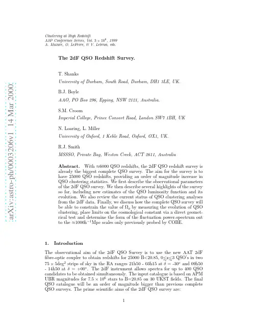
a rXiv:as tr o-ph/326v114Mar2Clustering at High Redshift ASP Conference Series,Vol.3×108,1999A.Mazure,O.LeFevre,&V.Lebrun,eds.The 2dF QSO Redshift Survey.T.Shanks University of Durham,South Road,Durham,DH13LE,UK.B.J.Boyle AAO,PO Box 296,Epping,NSW 2121,Australia.S.M.Croom Imperial College,Prince Consort Road,London SW71BH,UK N.Loaring,ler University of Oxford,1Keble Road,Oxford,OX1,UK.R.J.Smith MSSSO,Private Bag,Weston Creek,ACT 2611,Australia Abstract.With ≈6000QSO redshifts,the 2dF QSO redshift survey is already the biggest complete QSO survey.The aim for the survey is to have 25000QSO redshifts,providing an order of magnitude increase in QSO clustering statistics.We first describe the observational parameters of the 2dF QSO survey.We then describe several highlights of the survey so far,including new estimates of the QSO luminosity function and its evolution.We also review the current status of QSO clustering analyses from the 2dF data.Finally,we discuss how the complete QSO survey will be able to constrain the value of Ωo by measuring the evolution of QSO clustering,place limits on the cosmological constant via a direct geomet-rical test and determine the form of the fluctuation power-spectrum outto the ≈1000h −1Mpc scales only previously probed by COBE.1.IntroductionThe observational aim of the 2dF QSO Survey is to use the new AAT 2dF fibre-optic coupler to obtain redshifts for 25000B <20.85,0∼<z ∼<3QSO’s in two75×5deg 2strips of sky in the RA ranges 21h50-03h15at δ=-30◦and 09h50-14h50at δ=+00◦.The 2dF instrument allows spectra for up to 400QSO candidates to be obtained simultaneously.The input catalogue is based on APM UBR magnitudes for 7.5×106stars to B=20.85on 30UKST fields.The final QSO catalogue will be an order of magnitude bigger than previous complete QSO surveys.The prime scientific aims of the 2dF QSO survey are:121.To determine the QSO clustering power spectrum,P(k),in the range ofspatial scales,0∼<r∼<1000h−1Mpc.2.To measureΩΛfrom geometric distortions in clustering.3.To trace the evolution of QSO clustering in the range,0∼<z∼<3,to obtainnew limits onΩ0and QSO bias.Other aims include determining the evolution of the QSO LF evolution to z=3,cross-correlating the QSO’s with2dF Galaxy Survey groups to measureΩ0 via gravitational lensing(cf.Croom&Shanks,1999a)and constrainingΩΛby finding the sky density of close(6-20′′)lensed QSO pairs.Previous QSO clustering results have generally been based on the following complete QSO surveys-the Durham/AAT survey of Boyle et al(1988)com-prising392B<21QSO’s,the CFHT survey of Crampton et al(1989)with215 B<20.5QSO’s,the ESO survey of Zitelli et al(1992)with28B<22QSO’s, the LBQS survey of Hewett et al(1995)with1053B<18.8QSO’s and the ESO survey of LaFranca et al(1998)with300B<20.5QSO’s.These have produced results on QSO clustering at small(r<10h−1Mpc)scales which are consistent with an r−1.8power-law with amplitude r0≈6h−1Mpc which shows no evolution in comoving coordinates(Shanks et al1987,Andreani&Cristiani,1992,Shanks &Boyle,1994,Georgantopoulos&Shanks,1994,Croom&Shanks,1996).At larger scales(10<r<1000h−1Mpc),no clustering has previously been detected inξqq.2.2dF QSO Redshift Survey Status and Current Results.We now have redshifts for≈6000QSO’s where5600QSO’s have been observed using2dF itself.A further400QSO’s selected from the input catalogue have been observed on different telescopes for associated projects.Observations have included bright17<B<18.25QSO’s using UK Schmidt Telescope FLAIRfibre coupler,radio-loud QSO’s identified in the NRAO VLA Sky Survey(NVSS) and observed at Keck andfinally30QSO’s in close pairs(<20′′)from the ANU 2.3-m telescope.This makes the2dF survey already the biggest,complete QSO survey by a factor of≈6.From these observations,we know that53.5%of candidates are QSO’s which means there will be26000QSO’s infinal survey.The QSO number count,n(B), has been found to be in good agreement with previous surveys.The QSO redshift distribution,n(z),extends to z≈3because of our multi-colour UBR selection.In Fig.1we show the current Northern and Southern redshift cone plots from the 2dF survey.The rectangles shows the sky distribution of thefields that have already been observed.We have detected8close(<20′′)QSO pairs.Only one is a candidate gravitational lens;the separation is≈16′′(see Fig.6of Croom et al.,1999).The new2dF results for the QSO Luminosity Function continue to be consis-tent with Pure Luminosity Evolution models throughout the range0.35<z<2.3 (Boyle et al.,1988,1991,1999a).The luminosity function based on the current ≈6000QSOs of the2dF survey combined with≈1000LBQS QSOs are shown in Fig. 2.The large sample size makes it possible to define the QSO Luminosity3Figure1.The distribution of≈6000QSO’s with currently measuredredshifts in the2dF QSO Redshift Survey.The right-hand wedge isthe NGP area atδ=0◦,while the left-hand wedge is the SGP regionatδ=−30◦.The rectangular strips show the survey’s current skycoverage.Function in much smaller redshift bins than used previously and the accuracy of pure luminosity evolution as a description of QSO evolution is clear.Indeed,thisaccuracy is so high that it has prompted a new investigation of pure-luminosity evolution as a physical,as well as a phenomenological,model for QSO evolution. (Done&Shanks,1999,in prep.)The most interesting individual QSO that has been discovered from the2dF QSO survey is UN J1025-0040,a unique,post-starburst radio QSO at z=0.634,identified in the2dF-NVSS catalogue and followed up spectroscopically at the Keck(Brotherton et al.,1999).As well as broad emission lines,the spectrum also shows strong Balmer absorption lines indicative of a post-starburst galaxy.The starburst component of the spectrum at M B=-24.7dominates the AGN continuum spectrum by≈2mag.This2dF-NVSS collaboration has previously also uncovered a new class of radio-loud BAL QSO’s(Brotherton et al.,1998)and clearly has great potential for further exciting discoveries.Finally,we present a preliminary2dF QSO correlation function from ourmost complete subset of4115QSO’s.We have taken into account the current incompleteness of the2dF survey as best we can;however,this process is com-plicated by the fact that many observed areas still have overlapping2dF‘tiles’as yet unobserved.We show the preliminary correlation function in Fig.3(a) as a log-log plot and in Fig.3(b)as a log-linear plot.As can be seen the cor-relation function is consistent with being a-1.8power-law with r0≈4h−1Mpc and in good agreement with previous results(eg Croom and Shanks,1996).The QSO correlation function thus appears to be remarkably similar to the corre-lation function for local,optically selected galaxies and continues to show no evolution in comoving coordinates.This behaviour is consistent with evolution4Figure2.The2dF+LBQS QSO Luminosity Function based on≈6000QSO’s for a q0=0.5,H0=50kms−1Mpc−1cosmology.Incom-pleteness at M B>−23is due to host galaxy contamination.due to gravitational clustering either in a lowΩ0model or in a biased,Ω0=1 model.The correlation function is consistently positive out to about20h−1Mpc at3σand out to about50h−1Mpc at1σ,thus giving a hint of power extending to larger scales.At r>50h−1Mpc the errors inξare now as low as±0.016. There is also a suggestion of anti-correlation at r≈100h−1Mpc but still only at 1.5σsignificance.At all scales in the range100<r<1000h−1Mpc the correlation function is within1σof zero.3.Future Results.We have used mock catalogues drawn from simulations using the Zeldovich ap-proximation to demonstrate the accuracy of P(k)estimates at large scales that will be obtainable from the full survey(Croom et al.,in prep.).The results from this simulation show that our estimates of the power spectrum can recover the input spectrum up to scales of several hundreds of Mpc(k≈0.01hMpc−1)where the power spectrum is expected to turn over to its primordial form(see Boyle et al.,1999b).We are now using the Hubble Volume N-body simulation from the Virgo Consortium with of order109particles to produce mock QSO survey catalogues. We have‘light cone’output for a model withΩΛ=0.7,Ω0=0.3andσ8=1.0to test the potential of the geometric test of Alcock&Paczynski(1979)forΩΛdirectly in a biasedΛCDM model(Hoyle et al.,1999in prep.).We shall be using these simulations to see how robust the test is against different models for the bias.Constraints on these bias models come from the QSO-galaxy cross-corrrelation function(Ellingson et al.,1991,Smith et al.,1995,Croom&Shanks, 1999b)which suggest radio-quiet QSO’s inhabit similar environments to average5-0.100.10.20.30.40.51101001000ξr (h -1Mpc)0.0010.010.11101101001000ξr (h -1Mpc)Figure 3.(a)The 2-point auto-correlation function for 4115QSO’s from the 2dF QSO redshift Survey (closed circles),measured in co-moving coordinates with q 0=0.5.The open circles are the combined results from previous surveys (Croom &Shanks,1996).The line is a -1.8power law with r 0=4h −1Mpc.(b)2dF QSO correlation function as in (a).The line is a -1.8power law with r 0=4h −1Mpc which fits out to ≈50h −1Mpc.galaxies out to z=1.5.We are now extending QSO environment tests out to z ≈2using the INT Wide Field Camera at B <26and the AAT Taurus Tunable Filter (Croom &Shanks,in prep.)and these results will further constrain possible models of QSO bias at high redshift.4.Conclusions1.The 2dF QSO Survey has obtained redshifts for 6000/26000B <20.85,z <3QSOs which means it is already the biggest complete QSO survey by a factor of ≈6.2.Previous surveys detected QSO clustering at 4σlevel for r <10h −1Mpc where the QSO clustering appears stable when measured in comoving co-ordinates,suggesting either a low Ω0model or a biased,Ω0=1model.Previous surveys detected no significant clustering in ξqq at larger scales.3.The 2dF QSO survey confirms the accuracy of the PLE model of Boyle et al (1991)for the evolution QSO Luminosity Function for 0<z <2.2.4.The 2dF QSO survey has already detected many individually interesting objects,including a post-starburst QSO and several close QSO pairs.5.A preliminary 2dF QSO correlation function based on 4115QSOs shows results consistent with previous surveys and consistent with the correlation function of local,optically selected galaxies but with a hint of extended power to ≈50h −1Mpc.66.Mock catalogues from the Hubble Volume suggest the2dF QSO surveywill be able to determine QSO power spectrum out to∼>1000h−1Mpc and so detect the expected turnover to the primordial,n=1,slope.7.The potential of2dF QSO survey to constrainΩΛfrom both geometricdistortions and gravitational lensing is being tested in the Hubble Volume mock catalogues.Acknowledgments.We thank Fiona Hoyle,Carlton Baugh and Adrian Jenkins for allowing us to use the results from their analyses of the mock cat-alogues from the Hubble Volume simulation.The Hubble Volume is provided courtesy of the Virgo Consortium.ReferencesAlcock,C.&Paczynski,B.,1979,Nature,281,358.Andreani,P.&Cristiani,S.,1992,ApJ,398,L13.Boyle,B.J.,Shanks,T.&Peterson,B.A.,Mon.Not.R.astr.Soc.,1988,235, 935.Boyle,B.J.,Jones,L.R.,&Shanks,T.,1991.MNRAS,251,482.Boyle B.J.,Shanks,T.,Croom,S.M.,Smith,R.J.,Miller,L.,Loaring N.& Heymans,C.1999a,MNRAS,submitted.Boyle,B.J.,Smith,R.J.,Croom,S.M.,Shanks,T.,Miller,L.&Loaring,N., 1999b.Phil.Trans R.Soc.Lond.A.,357,185.Brotherton,M.S.,Van Breugel,Smith,R.J.,Boyle,B.J.,Shanks,T.,Croom, S.M.,Miller,L.&Becker,R.H.1998,ApJ,505,L7.Brotherton,M.S.,Van Breugel,W.Stanford,S.A.,Smith,R.J.,Boyle,B.J., Miller,L.,Shanks,T.,Croom,S.M.&Filippenko,A.V.,1999,ApJ,520, L87.Crampton,D.,Cowley,A.P.&Hartwick,F.D.A.,1989,ApJ,345,59.Croom&Shanks,1996,MNRAS,281,893.Croom,S.M.&Shanks,T.,1999a,MNRAS,307,L17.Croom,S.M.,Shanks,T.,Boyle,B.J.,Smith,R.J.,Miller,L.&Loaring,N.S., 1999.In”Evolution of Large Scale Structure:From Recombination to Garching”,eds.Banday,A.J.&Sheth,R.K.E32.Croom,S.M.&Shanks,T.,1999b,MNRAS,303,4.Ellingson,E.,Yee,H.K.C.&Green,R.F.,1991,ApJ,371,49. Georgantopoulos,I.&Shanks,T.,1994MNRAS,271,773.Hewett,P.C.,Foltz,C.B.&Chaffee,F.H.,1995,AJ,109,1498.La Franca,F.,Andreani,P.&Cristiani,S.,1998,ApJ,497,529.Shanks,T.,Fong,R.,Boyle,B.J.&Peterson,B.A.,MNRAS,1987,227,739. Shanks,T.&Boyle,B.J.,1994,MNRAS,271,753.Smith,R.J.,Boyle,B.J.,&Maddox,S.J.1995,MNRAS,277,270.Zitelli,V.,Mignoli,M.,Zamorani,G.,Marano,B.&Boyle,B.J.,1992MNRAS, 260,925.。

1. 星空中的星系是宇宙中最神秘和美丽的景象之一。

然而，这些闪烁的光点背后隐藏着许多迷人的故事和奥秘。

本文将带您探索星系中那些令人惊叹的幕后故事，揭示它们的形成、演化和其他令人着迷的特征。

2. 首先，我们来谈谈星系的形成。

在宇宙大爆炸之后，物质开始聚集形成星系。

根据天文学家的研究，星系可以通过两种方式形成：自发形成和相互作用形成。

3. 自发形成是指星系内部的物质自己聚集形成。

这种形成过程需要数百万年，甚至数十亿年的时间。

恒星的引力起到了关键的作用，将周围的物质吸引到一起，形成了星系的核心。

4. 相互作用形成则是指两个或多个星系之间的互动导致新的星系形成。

这种情况通常发生在星系之间的碰撞或擦过时。

当两个星系靠近时，它们之间的引力相互作用会导致物质重新分布，并形成新的星系。

5. 星系的演化是一个复杂而长期的过程。

在星系形成之后，恒星会逐渐燃尽它们的燃料，导致它们膨胀成红巨星或爆炸成超新星。

这些恒星的生命周期对于星系的演化起着关键作用。

6. 此外，星系中的黑洞也是一个引人注目的特征。

超大质量黑洞是星系中心的巨大黑洞，它们的质量相当于数百万到数十亿个太阳质量。

这些黑洞会吸收周围的物质，形成一个称为活动星系核（AGN）的区域。

7. 活动星系核释放出巨大的能量，产生强烈的辐射。

这些辐射可以影响星系中其他恒星和行星的演化，并对星系的结构和形态产生影响。

因此，黑洞在星系的演化中扮演着重要的角色。

8. 还有一些星系具有非常特殊的性质，被称为星暴星系。

星暴星系是指以异常高速率形成新恒星的星系。

这些星系通常富含气体和尘埃，这些物质是新恒星形成的原料。

9. 星暴星系可以通过多种方式形成，例如星系之间的碰撞、擦过或其他形式的相互作用。

在这些事件中，星系内的物质会被激发并引发剧烈的恒星形成活动。

10. 最后，让我们来谈谈星系中隐藏的暗物质。

暗物质是一种无法直接观测到的物质，但根据宇宙学模型的预测，它占据了宇宙总质量的大部分。